Ultra-wideband based cooperative relative localization algorithm and experiments for multiple unmanned aerial vehicles in GPS denied environments

Abstract

This article puts forward an indirect cooperative relative localization method to estimate the position of unmanned aerial vehicles (UAVs) relative to their neighbors based solely on distance and self-displacement measurements in GPS denied environments. Our method consists of two stages. Initially, assuming no knowledge about its own and neighbors’ states and limited by the environment or task constraints, each unmanned aerial vehicle (UAV) solves an active 2D relative localization problem to obtain an estimate of its initial position relative to a static hovering quadcopter (a.k.a. beacon), which is subsequently refined by the extended Kalman filter to account for the noise in distance and displacement measurements. Starting with the refined initial relative localization guess, the second stage generalizes the extended Kalman filter strategy to the case where all unmanned aerial vehicles (UAV) move simultaneously. In this stage, each unmanned aerial vehicle (UAV) carries out cooperative localization through the inter-unmanned aerial vehicle distance given by ultra-wideband and exchanging the self-displacements of neighboring unmanned aerial vehicles (UAV). Extensive simulations and flight experiments are presented to corroborate the effectiveness of our proposed relative localization initialization strategy and algorithm.

Introduction

Inter-unmanned aerial vehicle (UAV) relative localization (RL) is the pre-requisite for UAV teaming and swarming in the case when absolute localization information such as information from global positioning system (GPS) is unavailable or inaccurate,^1,2 which happens in indoor, urban, and forest environments. Therefore, RL is critically important in multi-UAV systems and there are pressing needs to study the inter-UAV RL problem.

A convenient solution for RL is to extract the distance and bearing information by using cameras. ³ However, cameras can only operate within a limited range and suffer greatly from occlusion and lighting conditions. On the other hand, distance measurement can be obtained from different types of sensing devices such as ultra-wideband (UWB), radars, and lidars, which can operate over a much larger range. In particular, UWB technology stands out in accurate ranging due to its ability to alleviate multi-path effects. Different from the space-sweep-ranging method of a widely used laser scanner, i.e. Hokuyo (≤30 m), UWB modules used herein are utilized for peer-to-peer ranging with bidirectional communications.

In this article, we focus on the active RL problem of determining the position of a moving UAV relative to its neighbors in a 2D plane through active sensing (measuring relative distance) and communications (exchanging self and neighbor’s displacements). Our proposed method constitutes two stages. Initially, without knowledge of its own and neighbors’ states, each UAV solves for an initial relative position estimate with respect to a static hovering UAV (a.k.a. beacon). To be specific, limited by the environmental space or task constraints, we aim to design some ranging path along which the moving UAV is able to effectively reduce its localization error. Particularly, the case of a moving UAV under motion constraint is considered, namely that the UAV can only move in a limited range. Such scenario is not rare when the UAV team is required to conduct cooperative tasks in a cluttered environment, say in a forest where neighboring UAVs are separated by trees. Besides, some specific task may require a quick solution of RL, which only allows a small movement.

Assuming noise-free displacement measurements, we reformulate the active RL problem as optimal sensor placement under constraint. Given the maximum allowed moving distance D, we manage to find the minimum mean square error (MMSE) in terms of D and the sample size n (the number of collected data for initialization). Based on this result, we then design a ranging path to effectively reduce the localization error. In the presence of displacement noise, we leverage the extended Kalman filter (EKF) to deal with the RL problem.

Starting with the refined initial RL estimate from the first stage, the second stage generalizes the EKF strategy to the case where all including beacon UAVs move simultaneously. In this stage, each UAV will transmit its displacement to its neighbors whenever a range request is triggered by any neighboring UAV. Thereupon, the self and neighbor’s displacements and their relative distance are fed into the proposed EKF estimator for updates.

The main contributions of the article are highlighted below:

A motion constraint RL is reformulated as an optimal sensor placement problem under constraint and according to theoretical analysis, an initialization stage for RL problem with the MMSE performance is designed.

A workable RL solution based on the EKF for miniature UAVs using light-weight UWB sensors (less than 60 g) is presented and extensive flight experiments in a large field (e.g. inter-UAV distance from 20 to 50 m) are conducted to verify our RL system.

The rest of the article is organized as follows. We first review some related works in “Related works” section, and formulate the problem in “Preliminaries and problem formulation” section. A rough initial RL estimate in the case of a single beacon is introduced in “RL with a single beacon” section and we analyze the corresponding MSE, based on which we, respectively, design the RL algorithm in both the cases of noise-free and noise-corrupted displacements. A cooperative RL method for simultaneous movements is presented in “Cooperative RL without beacon” section. Simulations and experiments are conducted, respectively, in “Simulation results” and “Experiments with UAVs” sections and verify our approach, and we conclude our work in “Conclusion and future work” section.

Related works

In general, the main RL algorithms are classified into two categories: beacon-based and beacon-free. In this article, the proposed single beacon based RL (first stage) serves as the initialization of the beacon-free RL (second stage). Furthermore, a motion constraint, which is reformulated herein as optimal sensor placement under constraint, is considered in the first stage. The related works are introduced as follows.

RL with a single beacon

In the case of a static beacon, the RL problem can be viewed as a source localization problem. By treating the source location in 3D space as parameters to be estimated and assuming exact distance and self-position measurements, Dandach et al. ⁴ proposed a continuous-time adaptive method to achieve the exponential convergence of the location estimation, given that the mobile agent regularly avoids the planar motion.

By including the distance measurement as an augmented state, Batista et al. ⁵ transformed the original nonlinear system of the source location into a linear time-varying system and applied Kalman filter for its location estimation. The necessary motion to guarantee a convergent estimate was given by analyzing the observability of the time-varying system. A similar method was also adopted in the discrete-time case Batista et al. ⁶ With a periodic motion of the mobile agent, a recursive least squares fading memory filter was applied to the squared distance measurements in Indiveri et al. ⁷ However, note that the above approaches require the agent to move a long distance before getting a convergent solution, and the design of a ranging path to effectively reduce error is not considered. Also, the squaring of distance measurements may result in a larger estimation error. Mueller et al., ⁸ who is the earliest adopter of UWB for quadcopter state estimation and control, utilized accelerometers, gyroscopes, and UWB radios to estimate the dynamic state of a quadrocopter and flight tests were successfully conducted along a 4 m × 3 m horizontal rectangle. However, five UWB radios had to be used as anchors for only one quadrocopter localization and the dynamic model of this quadrocopter was necessarily required. Wang et al. ⁹ novelly combined moving horizon estimate (MHE) and convex optimization to perform 3D multirobot localization with constraints and unknown initial poses. However, this method was applied in a centralized manner and suffered from a heavy computational burden. Therefore, at present, it is difficult to be implemented on multiple miniature UAVs.

Cooperative RL

Based on rigidity theory, a robust quadrilaterals algorithm, Moore et al. ¹⁰ was proposed to cope with landmark-free localization using distance measurements between agents. More recently, Diao et al. ¹¹ developed a generalized barycentric coordinate representation and algorithm for determining the sensor locations in a randomly deployed sensor network and this method was implemented in an iterative and distributed manner. These methods seem close in spirit to our work. However, these algorithms aimed primarily at static sensor networks. The majority of work on localization generally either require stationary nodes or are not limited to range only measurements for static sensor networks.^12–14

Localization for mobile robots in 2D using range only measurements have been demonstrated in literature.^15–18 In these works, the relative position between robots is estimated after the robots travel through a sequence of positions and orientations where the experimental verifications were not considered therein. Recently, an on-board Bluetooth-based RL method is proposed by Coppola et al. ¹⁹ for collision avoidance in UAV swarms. In practical tests, three UAVs (using offline velocity estimate) or two UAVs (using on-board optical flow) flying in a 4 m × 4 m space collided once over a cumulative flight-time of around 3 min as a result of the disturbances of the on-board velocity estimate. Note that, in this latest research result, the flight tests were conducted only in a small space due to the limitation of Bluetooth signals. By using UWB signals, our proposed system can operate within at least a 100-level ²⁰ region.

In our work, for the first stage, we adopt a similar approach as in the optimal sensor placement problem to solve the active initial RL problem under the constraint of the UAV’s motion. Actually, assuming an accurate self-displacement measurement, solving the RL problem is equivalent to estimating the relative position at the starting point, and the motion constraint can be projected on the sensor configuration. As a result, the active RL problem is reformulated as a constrained optimal sensor placement and we seek the optimal configuration to minimize the estimation error bound under the constraint. As shown later in Theorem 4.1, the lower error bound is dependent on the maximum allowed moving distance D and the sample size n, and hence one only needs to enlarge the ranging span to effectively reduce the estimation error. Such an idea will be applied to the design of ranging path, as seen in the Error analysis section. In the second stage, starting with the initial RL guess from the first stage, an EKF strategy is proposed to dynamically sustain the RL estimation and deal with the noise in distance and displacement measurements. Besides, in the literature, most of the works focus on the RL algorithm design. Field experiment solutions especially for miniature UAVs are rare.

Preliminaries and problem formulation

For convention, we use vector $p$ and $\chi$ to represent the global position and relative position, respectively. For instance, $\chi \mathrm{ij}=P_i{P}_j=p_j-p_i=(x_{j,k}-x_{i,k},y_{j,k}-y_{i,k})$ represents the relative coordinate between UAVi and UAVj in an agreed frame (e.g. North-East plane). $\hat{\chi }$ denotes an estimate of $\chi$ and $\Vert \chi \Vert$ represents the relative distance.

Before delving into details, it is necessary to state the UWB based indirect cooperative RL problem. We consider a team of mobile UAVs labeled $1,2,\dots N$ in Figure 1(a). The problem is to estimate the relative position of each UAV to their neighbors. Suppose that each UAVi is able to access its own displacement $\delta p_i(\Delta x_i,\Delta y_i)$ and has distance measurements between it and its neighbors UAVj, i.e. $d_{\mathrm{ij}}=\Vert \chi \mathrm{ij}\Vert$ as shown in Figure 1(b). The goal is to estimate the inter-UAV relative coordinate $\chi \mathrm{ij}$ based on distance measurements and displacement information exchanged with neighbors using UWB sensors installed on each UAV. For each UAVi, denote the set of its neighbors by ${\mathcal{N}}_i$ , which means $j\in {\mathcal{N}}_i$ if UAVi is able to range with UAVj and UAVj can transmit its displacement $(\Delta x_j,\Delta y_j)$ and height (for transforming a 3D distance measurement into 2D) to UAVi through UWB radio.

Figure 1.

Distances, displacements, and relative position of three UAVs during simultaneous movement.

RL with a single beacon

Initial relative position estimation

To achieve an accurate RL estimate, we first assign one static UAV as a beacon while other UAVs range to and communicate with it. In this section, we shall formulate the problem in the perspective of nonlinear least squares (NLS).

As shown in Figure 2, O is the location of the static beacon and the mobile UAV starts from P₀ and takes the distance measurement d_i at each point P_i, $i=0,\dots ,n$ . RL aims to estimate the vector ${\mathrm{OP}}_0$ from the displacements $P_0{P}_i$ , as well as the distance measurement r_i. Denote $p_0={\mathrm{OP}}_0=(x_0,y_0),\Delta p_i=P_0{P}_i=(\Delta x_i,\Delta y_i)$ , and $d_i=f_i(x_0,y_0)=\Vert {\mathrm{OP}}_i\Vert =\sqrt{(x_0+\Delta x_i)2+(y_0+\Delta y_i)2}$ . To simplify the analysis, we assume that the displacement measurements are free of noise and the distance measurements are corrupted by independently and identically distributed noises, i.e. $r_i=d_i+{\eta }_{r,i}$ , where $E{\eta }_{r,i}=0,E{\eta }_{r,i}{\eta }_{r,j}=0$ for all $i\ne j$ and $E{\eta }_{r,i}^2=\sigma 2$ . Consequently, we only need to estimate $p_0$ by solving the NLS problem, i.e.

$${min}_{x_0,y_0}\sum _{i=0}^n(r_i-f_i)2$$

(1)

Figure 2.

Relative localization to a static beacon.

Denote ${\hat{p}}_0=({\hat{x}}_0,{\hat{y}}_0)$ as the position estimate, ${\hat{f}}_i=f_i({\hat{x}}_0,{\hat{y}}_0),{\hat{p}}_i=({\hat{x}}_i,{\hat{y}}_i)={\hat{p}}_0+\Delta p_i$ and ċ as the inner product of two vectors. The solution to the above problem can be obtained by using Gauss–Newton method Björck, ²¹ which is based on the linear approximation of f_i around the current estimate $({\hat{x}}_0,{\hat{y}}_0)$ as

$$f_i\approx {\hat{f}}_i+\frac{1}{{\hat{f}}_i}({\hat{x}}_0+\Delta x_i,{\hat{y}}_0+\Delta y_i)·(x_0-{\hat{x}}_0,y_0-{\hat{y}}_0)$$

(2)

and solving the corresponding normal equation

$$(r_0-{\hat{f}}_0{r}_1-{\hat{f}}_1:r_n-{\hat{f}}_n)=({\hat{x}}_0/{\hat{f}}_0{\hat{y}}_0/{\hat{f}}_0{\hat{x}}_1/{\hat{f}}_1{\hat{y}}_1/{\hat{f}}_1::{\hat{x}}_n/{\hat{f}}_n{\hat{y}}_n/{\hat{f}}_n)(x_0-{\hat{x}}_0{y}_0-{\hat{y}}_0)$$

(3)

The above equation can be rewritten as $\Delta r({\hat{p}}_0)=H(\widehat{p_0})\Delta \kappa$ and $\Delta \kappa$ is found as

$$\Delta \kappa =(H’H)-1H’\Delta r$$

(4)

If $H$ is of full column rank, the newly obtained estimate ${\hat{p}}_0\leftarrow {\hat{p}}_0+\Delta \kappa$ can be used to update $H$ and $\Delta r$ , respectively, for the next iteration until $\Delta \kappa$ is sufficiently small.

Remark 4.1

An initial guess is needed to solve (1), which comes from the solution of a related linear least squares problem with the squared distances Navidi et al. ²² To be exact, the distance measurements r_i is corrupted by noise. However, to achieve an initial guess, we temporarily assume that r_i is equal to d_i regardless of noise, i.e. $r_i=\sqrt{(x_0+\Delta x_i)2+(y_0+\Delta y_i)2}$ . Consequently, by squaring both sides of that and subtracting the first equation $r_0^2=x_0^2+y_0^2$ , we get the following linear system:

$$2[\Delta x_1\Delta y_1\Delta x_2\Delta y_2::\Delta x_n\Delta y_n][x_0{y}_0]=[r_1^2-r_0^2-(\Delta x_1^2+\Delta y_1^2)r_2^2-r_0^2-(\Delta x_2^2+\Delta y_2^2):r_n^2-r_0^2-(\Delta x_n^2+\Delta y_n^2)]$$

(5)

or $2{\mathrm{Ap}}_0=\Delta d$ . Now an initial guess of $p_0$ is given by

$${\hat{p}}_0=\frac{1}{2}(A’A)-1A’\Delta d,$$

(6)

as long as $A$ has full column rank, or equally the n points P_i’s ( $i=1,\dots ,n$ ) are not along the same line.

Remark 4.2

Although equation (5) is able to give an exact solution when there is no ranging error, the introduction of squared distances would increase the error of calculation and only achieves a rough estimate in the presence of measurement noises. In fact, assume that the range measurement $r\hspace{1em}\sim N(\overline{r},\sigma 2)$ , then the variance of r² is given by $4\overline{r}2\sigma 2+2\sigma 4$ , which is dependent on $\overline{r}2$ . In contrast, (3) employs the original measurements as the input and a rough initial guess is able to guarantee the convergence to a more accurate solution in just a few iterations. Hence, we employ the rough estimate of (6) as the initial guess for solving (1) and obtain a refined estimate from Gauss–Newton (GN) method. The process of solving the rough initial RL guess is summarized in Algorithm 1.

Algorithm 1

NLS-GN based Initial Relative Estimation

1: procedure Initial Relative Estimation

2: Collect rangings and produce relative localization:

3: Starting from P₀, the UAV moves along some nonlinear path as described in Error analysis section and collects n distance measurements r_i.

4: Calculate rough initial estimate:

5: Form the linear equations as (5) based on the overall available ranging measurements r_i and $\Delta p_i$ .

6: calculate an initial rough estimate ${\hat{p}}_0=({\hat{x}}_0,{\hat{y}}_0)$ using (6).

7: Improve rough initial estimate:

8: Set the maximum iteration step as S and the positive threshold of estimation error as ε.

9: for $k\leftarrow 1\text{to}S$ do

10:  Calculate GN iteration (4) $\to \Delta \kappa$

11:   ${\hat{p}}_0\leftarrow {\hat{p}}_0+\Delta \kappa$

12:  if $\left|\Delta \kappa \right|\le \epsilon$ then break;

13:  end if

14: end for

15: end procedure

Error analysis

In the sequel, we seek to find a lower bound of the estimation error of the problem (1) as well as the corresponding path configuration, given that the mobile UAV can only move by a maximum distance of D in the whole duration of RL. The optimum configuration then serves to guide the design of the ranging path, in an effort to effectively reduce the estimation error under the motion constraint.

In this section, we shall first analyze the RL error based on (4) to find its lower bound of MSE, and then propose an effective sampling strategy to reduce the error. Two different cases are studied, depending on whether or not the displacement measurements are corrupted by noise.

By (4), the error covariance matrix can be approximated by

$$E=\sigma 2(H’H)-1$$

(7)

Rewrite $H=[\mathrm{cs}]$ and denote $[{\hat{x}}_i/{\hat{f}}_i{\hat{y}}_i/{\hat{f}}_i]=[\cos {\theta }_i\sin {\theta }_i]$ for each row in $H$ , where θ_i is shown in Figure 2. Then $(H’H)-1$ is obtained as

$$(H’H)-1=\frac{1}{det(H’H)}[s’s-c’s-c’sc’c]$$

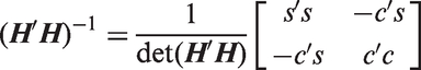
Now the MSE is given by the trace of E as

$$\mathrm{MSE}=\frac{\sigma 2(n+1)}{det(H’H)}$$

(8)

where n + 1 is the number of distance measurements. Direct computation shows that

$$det(H’H)=\sum _{i\ne j}\cos 2{\theta }_i\sin 2{\theta }_j-\sum _{i\ne j}\cos {\theta }_i\sin {\theta }_i\cos {\theta }_j\sin {\theta }_j=\sum _{i\ne j}(\cos 2{\theta }_i\sin 2{\theta }_j-\cos {\theta }_i\sin {\theta }_i\cos {\theta }_j\sin {\theta }_j)=\sum _{i\ne j}(\cos {\theta }_i\sin {\theta }_j-\cos {\theta }_j\sin {\theta }_i)2=2\sum _{0\le i<j\le n}\sin 2({\theta }_i-{\theta }_j)$$

(9)

Remark 4.3

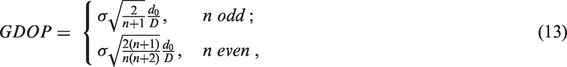
Note that the error covariance matrix E is also the Cramer–Rao lower bound, or the inverse of the Fisher Information Matrix (FIM). In the GPS literature, the squared root of the MSE is defined as the geometric dilution of precision (GDOP) Levanon. ²³

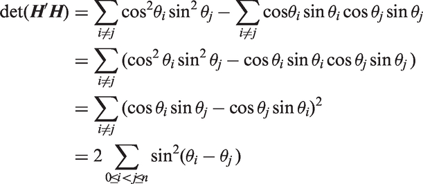
Given a fixed number of range measurements to minimize MSE is to maximize the cost function

$$J=2\sum _{0\le i<j\le n}\sin 2({\theta }_i-{\theta }_j)$$

(10)

Denote $\Theta =\arcsin (D/d_0)$ as the largest angle spanned by the mobile UAV within the moving radius as shown in Figure 3(b) and assume that $\Theta \le \frac{\pi }{4}$ , or equivalently $D\le d_0\sin \frac{\pi }{4}=\frac{\sqrt{2}}{2}{d}_0$ . Obviously, we can always sort θ_i’s in an ascending order, and ${\theta }_0$ can be selected to be 0 (as shown in Figure 3(a)) after proper rotation without changing the determinant. Moreover, when $0\le {\theta }_i\le \Theta \le \frac{\pi }{4}$ , it can be seen that the maximum of J dictates the largest angle ${\theta }_n=\Theta$ . To summarize, we try to solve the problem

$${max}_{{\theta }_i\in G}\sum _{0\le i<j\le n}\sin 2({\theta }_i-{\theta }_j)$$

(11)

where $G=\{({\theta }_0,{\theta }_1,\dots ,{\theta }_n):0={\theta }_0\le {\theta }_1\le \dots \le {\theta }_n=\Theta \le \frac{\pi }{4}\}$ is a closed convex region. We have the following result:

Theorem 4.1

Assume that the maximum allowed moving distance $D\le \frac{\sqrt{2}}{2}{d}_0$ . Then (11) is solved if ${\theta }_0=\dots ={\theta }_{\lfloor \frac{n}{2}\rfloor }=0$ and ${\theta }_{\lfloor \frac{n}{2}\rfloor +1}=\dots ={\theta }_n=\Theta$ , where $\lfloor \frac{n}{2}\rfloor$ denotes the biggest integer no greater than $\frac{n}{2}$ .

Figure 3.

Angle tags and maximum ranging span within the moving radius.

Correspondingly,

$$maxJ=\{\frac{(n+1)2}{2}(\frac{D}{d_0})2,\mathrm{nodd};n(\frac{n}{2}+1)(\frac{D}{d_0})2,\mathrm{neven}.$$

(12)

Proof

Notice that each individual term is the squared sine of a linear function of $({\theta }_0,{\theta }_1,\dots ,{\theta }_n)$ , and $y=\sin 2\theta$ is increasing and convex over $[0,\frac{\pi }{4}]$ . Therefore, each individual term $\sin 2({\theta }_j-{\theta }_i)$ is a convex function for $0\le {\theta }_i\le {\theta }_j\le \frac{\pi }{4}$ Hiriart-Urruty and Lemaréchal, ²⁴ and so does the summation J. As a result, the maximum of J on the closed convex region G is obtained at the extreme points of G, namely those with ${\theta }_i=0$ or Θ for $i=1,\dots ,n-1$ . The rest follows naturally.

Remark 4.4

From the above result, we can see that the localization error is dependent on the maximum spanning angle Θ, as well as the sample size. Intuitively, a larger field of view and more distance measurements help reduce the localization error. By (12) and (8), we can see that

$$\mathrm{GDOP}=\{\sigma \sqrt{\frac{2}{n+1}}\frac{d_0}{D},\mathrm{nodd};\sigma \sqrt{\frac{2(n+1)}{n(n+2)}}\frac{d_0}{D},\mathrm{neven},$$

(13)

which extends the result of lowest $\mathrm{GDOP}=\sigma \sqrt{\frac{2}{n+1}}$ when there is no restriction on the sensor placement Levanon. ²³

RL algorithm with a single beacon

Noise-free case

From Remark 4.4, we know that the key point of reducing localization error is to enlarge the spanning angle between ${\mathrm{OP}}_0$ and ${\mathrm{OP}}_n$ . Clearly, if the relative position p ₀ can be known exactly, then the UAV only needs to move in the straight line along the optimal direction to the peripheral in an effort to maximize the span. However, due to the inaccurate position estimate, we need to adaptively determine the heading to enlarge the span as much as possible. Besides, as mentioned in Remark 4.1, a nonlinear path is also needed to initialize the estimation. Bearing these in mind, we propose a two-phase algorithm to actively reduce the localization error as follows, which consists of a nonlinear path of length D₁ and a piecewise linear path of length D₂ with the total traveling distance $D=D_1+D_2$ . Also see Figure 4 for clarification.

Algorithm 2

Two-phase Active RL (TPARL)

Figure 4.

Two-phase active RL with a single beacon.

1: procedure TPARL

2: Phase I (Nonlinear): Starting from P₀, the UAV moves along some nonlinear path of length D₁ collecting distance measurements, and produce an initial rough estimate ${\hat{p}}_0=({\hat{x}}_0,{\hat{y}}_0)$ following as Algorithm 1 in RL algorithm with a single beacon.

3: Phase II (Piecewise linear): Assume that the mobile UAV is to move N steps of linear path of fixed length l and $\mathrm{Nl}\le D_2$ .

4: for $i\leftarrow 1\text{to}N$ do

5:   $\hat{\theta }\leftarrow \arcsin (l/r_0)$

6:   $\hat{\lambda }\leftarrow \arctan 2({\hat{y}}_0,{\hat{x}}_0)$

7:   $\alpha \leftarrow \hat{\lambda }-\hat{\theta }-\frac{\pi }{2}$ (in North-East frame)

8:  Move along a straight line with the heading α

9:  Collect new rangings and produce new estimate ${\hat{p}}_0=({\hat{x}}_0,{\hat{y}}_0)$ by GN method (Algorithm 1) from the overall rangings and displacements

10: end for

11: end procedure

Remark 4.5

Several points have to be noted from the above algorithm. The first is the choice of length of the nonlinear path. Although an initial guess can be generated from three samples on a nonlinear path as seen from (5), the estimation error may be so large that a refined estimate in phase II may have a counter direction to that of the rough estimate, thus reduce the ranging span as a whole. Therefore, the nonlinear path should be long enough to guarantee a relatively accurate initial estimate. The second point is with regard to the choice of the shape of the nonlinear path. Notice that we assume no prior knowledge of the relative position $p_0$ , the nonlinear path should avoid the case where the path is relatively monotonous when viewed along the direction of $p_0$ and incurs a lost of ranging span. Hence, in the follow-up simulation and experiment, we take a square path. Third, by Theorem 4.1 and Figure 3 , we note that samples should be taken at the extreme points to reduce error. However, considering that such a maneuver incurs frequent stops, which not only increases the RL duration but also consumes extra energy, and the sampling at the extreme points for a short path will only make a slight improvement to RL estimation, we do not apply such a strategy in the piecewise linear phase. Instead, we only focus on how to enlarge the ranging span from the baseline $p_0$ , as seen from the for-loop in phase II.

Remark 4.6

It should be noted that each change of heading actually serves to maximize the span from the initial position to the next waypoint based on the newest relative position estimate, and is only needed when there is a much different estimate from the last one. For simplicity, here we set a fixed length movement for each step, but it can be variable in practice.

Noise-corrupted case

In this subsection, we consider the design of EKF for the same strategy as that of the case without noise to take the displacement noise into account and the initial RL estimate from Algorithm 2 will be fed into the proposed EKF for the first step calculation. The sampling algorithm remains the same, while the estimate is provided by EKF.

For the EKF design, we need to determine the state equation and observation equation. The state space representation consists of the initial relative position $p_{0,k}$ and the displacement $\Delta p_k$ , with the system dynamics given as follows:

$$\{p_{0,k+1}=p_{0,k}+{\xi }_{p_0,k},\Delta p_{k+1}=\Delta p_k+u_k+{\xi }_{u,k},$$

(14)

where $u_k$ is the position increment from time step k to k + 1 provided by the on-board navigation system, and ${\xi }_{u,k}$ is the related white noise. Note that the term ${\xi }_{p_0,k}$ denotes the possible perturbation of the beacon, e.g. a hovering UAV or a floating buoy, which can be seen as white noise, and ${\xi }_{p_0,k}\equiv 0$ if the beacon keeps static.

On the other hand, the observation consists of the relative range r_k, and the displacement $z_k$ from the starting P₀ as below:

$$\{r_k=\Vert p_{0,k}+\Delta p_k\Vert +{\eta }_{r,k},z_k=\Delta p_k+{\eta }_{z,k},$$

(15)

where ${\eta }_{r,k}$ and ${\eta }_{z,k}$ are the corresponding white noises. Note that the only nonlinear part of the system comes from the relative range r_k, which needs to be linearized in the EKF.

Remark 4.7

In the state equation (14), we split the relative position into the initial relative position $p_0$ and the displacement $\Delta p$ . For one thing, we need the estimate of $p_0$ to determine the heading at the next step as seen from the algorithm; for the other, the inclusion of $\Delta p$ in the filter helps improve the navigation of the mobile UAV.

Cooperative RL without beacon

In this section, we consider the case of a dynamic team as depicted in Figure 1, where the UAV serving as a “beacon” in RL algorithm with a single beacon is also mobile. For any two team members, say UAVi and UAVj, their kth relative position estimate ${\chi }_k^{\mathrm{ij}}$ is to be estimated, $k\in \mathbb{N}$ at time $t=t_k$ according to ${\chi }_k^{\mathrm{ij}}=P_{i,k}{P}_{j,k}=(x_{j,k}-x_{i,k},y_{j,k}-y_{i,k})$ . For brevity, we denote ${\chi }_k^{\mathrm{ij}}=(X_k,Y_k)=(X_0+\Delta X_k,Y_0+\Delta Y_k),{\chi }_0^{\mathrm{ij}}=(X_0,Y_0)$ and $\Delta {\chi }_k^{\mathrm{ij}}=(\Delta X_k,\Delta Y_k)$ , where $(\Delta X_k,\Delta Y_k)$ is the vector of the difference of the displacement from their respective launching point, namely $(\Delta X_k,\Delta Y_k)=\Delta P_{i,k}{P}_{j,k}=(\Delta x_{j,k}-\Delta x_{i,k},\Delta y_{j,k}-\Delta y_{i,k})$ . Then the distance d_k can be described as $d_k=\Vert {\chi }_k^{\mathrm{ij}}\Vert =\Vert {\chi }_0^{\mathrm{ij}}+\Delta {\chi }_k^{\mathrm{ij}}\Vert$ . A similar EKF structure as that in RL algorithm with a single beacon is proposed to account for the noise of the difference of the increment of UAVs’ displacements and their relative distances. The state space representation consists of the initial relative position ${\chi }_{0,k}^{\mathrm{ij}}$ and the difference of a pair of displacements $\Delta {\chi }_k^{\mathrm{ij}}$ , with the system dynamics given as follows: where ${\nu }_k$ is the difference of the displacements’ increment of UAVi and UAVj from time step k to k + 1. Assume the measurement noise of each UAV’s displacement $(\Delta x,\Delta y)$ is Gaussian with the distribution $N(0,\sigma 2)$ and independent with each other UAV’s displacement measurement. Then, we can get ${\zeta }_{\nu ,k}\hspace{1em}\sim N(0,2\sigma 2)$ .

The observation consists of the relative range r_k, and the displacement difference ${\rho }_k$ from the starting $P_{i,0}$ and $P_{j,0}$ as below:

$$\{r_k=\Vert {\chi }_{0,k}^{\mathrm{ij}}+\Delta {\chi }_k^{\mathrm{ij}}\Vert +{\eta }_{r,k},{\rho }_k=\Delta {\chi }_k^{\mathrm{ij}}+{\upsilon }_{\rho ,k},$$

(17)

where the displacement difference ${\rho }_k$ of UAVi and UAVj is different from (15).

Combined with the initial RL algorithm described in Algorithms 1 and 2, the proposed cooperative RL is summarized in Algorithm 3.

Algorithm 3

Cooperative localization without beacon

1: procedure Relative localization

2: Data communication: UAVi sends range request to its neighbor UAVj and receive this neighbor’s displacement and height information (which helps transfer a 3D distance measurement into 2D).

3: Data matching: The collected UAVj’s information and measured distance are stored together with UAVi’s displacement and height measurement by querying the closest UAVi’s sensor data in the buffer.

4: Based on the initial relative estimate (Algorithm 2) and selected historical data (e.g. m samples), execute m steps EKF as (14) and (15) to initialize the estimation of the states of UAVs for the simultaneous movement.

5: while $\mathrm{CooperativeFlight}$ do

6:    ${\hat{\chi }}_{0,k+1|k}^{\mathrm{ij}},\Delta {\hat{\chi }}_{k+1|k}^{\mathrm{ij}}\leftarrow (16)$

7: $H1=\frac{[({\hat{\chi }}_{0,k+1|k}^{\mathrm{ij}}+\Delta {\hat{\chi }}_{k+1|k}^{\mathrm{ij}})T,({\hat{\chi }}_{0,k+1|k}^{\mathrm{ij}}+\Delta {\hat{\chi }}_{k+1|k}^{\mathrm{ij}})T]}{{\hat{r}}_{k+1|k}}$

8:   $H2=[1_{2\times 2},0_{2\times 2}]$

9:   $H=[H1H2]$

10:  carry out EKF

11:  update ${\hat{\chi }}_{0,k+1}^{\mathrm{ij}}$ and $\Delta {\hat{\chi }}_{k+1}^{\mathrm{ij}}$

12:  calculate ${\hat{\chi }}_{k+1}^{\mathrm{ij}}={\hat{\chi }}_{0,k+1}^{\mathrm{ij}}+\Delta {\hat{\chi }}_{k+1}^{\mathrm{ij}}$

13: end while

14: end procedure

Simulation results

RL with a single beacon

In this section, the performance of the proposed distance-based active RL Algorithm 2 is evaluated by simulation, respectively, for the cases of noise-free and noise-corrupted self-displacements. Specifically, in the former case, we compare the performance of the proposed algorithm with that of a constant heading in the piecewise linear phase, in order to show the necessity of adaptive heading. Besides, we also compare the performance of our approach with that of other two methods in the literature.

For a comprehensive evaluation, the initial starting point P₀ is placed at different circles centered at O, over a span of radius from 20 to 50 m with an interval of 5 m, as seen from the abscissa in Figures 5 and 6. On each circle, P₀ will be randomly generated by the uniform distribution and 50 Monte–Carlo simulations are repeated, with the whole absolute localization error distribution on each direction represented in the form of box plot. Note that the blue box contains an approximate 95% of the data in case of Gaussian distribution, and the red one covers the data around the sample mean within one unit of standard deviation.

Figure 5.

Absolute error comparison between switching heading and constant heading in noise-free case. (a) Absolute estimation error with switching heading in noisefree case, (b) Absolute estimation error with constant heading in noisefree case.

Figure 6.

Absolute error comparison in noise-corrupted case. (a) Absolute estimation error of the proposed RL, (b) Absolute estimation error by including augmented state Batista et al. (2013), (c) Absolute estimation error by recursive least squares method Indiveri et al. (2012).

Some common parameters in the simulation are listed as follows. The UAV moves at the speed of 1 m/s, the ranging frequency is given by 5 Hz, and the ranging noise ${\eta }_{r,k}\hspace{1em}\sim N(0,0.12)$ . In both cases, the nonlinear path (phase I) is taken as a square of 1.5 m × 1.5 m, and the piecewise linear path (phase II) consists of six movements along each segment of 1 m. Therefore, the UAV will move 12 m in total, and it is noted that $12<\frac{\sqrt{2}}{2}\underset{¯}{d}$ with $\underset{¯}{d}=20\text{m}$ as the smallest distance in the simulation. In other words, the assumption of Theorem 4.1 is satisfied.

Noise-free case

With the noise-free displacement measurement, the RL problem is equivalent to estimating $p_0$ and the estimation error is the difference between $p_0$ and ${\hat{p}}_0$ . Figure 5(a) and (b) shows the absolute estimation error on each direction in the cases of switching and constant heading, respectively. In the latter case, the heading of the mobile UAV in phase II is fixed based on the estimate ${\hat{p}}_0$ at the end of phase I. From Figure 5(a), it can be seen that the estimation error tends to increase with the distance, with most of the estimation error falling within the bound of 0.4 m on each direction. In the worst case, the estimation error is still within 0.6 m. In comparison, we observe from Figure 5(b) that the sizes of error boxes are all larger than their counterparts in the switching heading case, ranging from 0.4 to 0.8 m, and in some extreme cases, the estimation error can be as large as 2.5 m. Obviously, the performance of Algorithm 2 is satisfactory if we consider the distance of 50 m and accuracy of 0.6 m in the worst case, with only a movement of 12 m. The comparison between Figure 5(a) and (b) also justify the necessity of changing heading to effectively reduce the localization error.

Remark 6.1

Note that the mean values of the estimation errors in the constant heading case are still less than 0.5 m. In practice, without strict accuracy requirements, we may simply fix the heading after the initial rough estimation and the RL estimates still can be accepted.

Noise-corrupted case

In this subsection, we evaluate the performance of EKF in RL algorithm with a single beacon when the displacement measurement is corrupted by noise. Under the assumption of ${\xi }_{u,k}\hspace{1em}\sim N(0,0.12)$ and ${\eta }_{z,k}\hspace{1em}\sim N(0,0.72)$ (see (14) and (15) for the noise definition with the standard deviations summarized from experiments), we redo the simulation under the same setting in RL algorithm with a single beacon and plot the result in Figure 6(a). Note that the absolute estimation error, in this case, is the average absolute error of RL over the whole ranging path. It can be seen that on each sampling circle, all the mean absolute estimation errors are bounded within 1 m on each direction, and most of the estimation falls within the error bound of 1.5 m.

Comparison with other methods

Here we compare the performance of our approach with that of Batista et al. ⁶ and Indiveri et al. ⁷ under the same setting in RL algorithm with a single beacon, as respectively shown in Figure 6(b) and (c). We can see that the absolute estimation error in Figure 6(b) generally ranges from 2 to 5 m, much larger than that in Figure 6(a), while the error in Figure 6(c) can be as large as dozens of meters. Such a poor performance when compared with the approach in this article can be expected, if we note that the augmented system in Batista et al. ⁶ requires more movement and samples to produce a convergent estimate, and the squared distance measurements result in an enlarged error and a poor estimate when the ranging path adopted in this article is not so nonlinear as that in Indiveri et al. ⁷

Cooperative RL without beacon

In this section, we will demonstrate the accuracy of the cooperative RL for 3 UAVs. In the simulation, the initial RL (with a single beacon) and its corresponding covariance are fed into the cooperative RL algorithm (without beacon) directly for the first step estimate. The noise of displacement difference ${\zeta }_{\nu ,k}\hspace{1em}\sim N(0,2\times 0.252)$ and distance noise ${\eta }_{r,k}\hspace{1em}\sim N(0,0.12)$ are added into our simulation. For consistency, all the parameters for initial RL estimate are adopted directly (as seen in Section 6.1). The flight time of initial RL is 12 s (phases I and II are set as 6 s and 6 s, respectively), and that of simultaneous movement (without beacon) is 600 s.

In practice, the relative position among UAVs is leveraged for achieving multi-UAV performance such as formation shape control, flocking, and coverage control, where the trajectory of each UAV is controlled by their behavior manager. To verify the proposed RL algorithm independently, a serpentine path of UAV1 is simply applied while UAV2 and UAV3 just fly straight and keep the same heading as that at the end of phase II (Algorithm 2). Besides, no control laws (e.g. obstacle avoidance, formation control, and path planning) are applied in the simulation.

The flight trajectories of three UAVs are depicted in Figure 7 and the statistic accuracy (350 tests as introduced in Section 6.1) of RL estimate during the simultaneous flight phase is shown in Figure 8. Figure 9 shows the indirect RL estimate of UAV3 to UAV2 ( $\chi 32$ ) generated by the RL estimates of UAV3 to UAV1 ( $\chi 31$ ) and UAV2 to UAV1 ( $\chi 21$ ).

Figure 7.

Flight trajectories of three UAVs for 600 s in noise-corrupted case.

Figure 8.

Absolute RL estimation error with measurement noise during the simultaneous flight phase (600 s) in Figure 7.

Figure 9.

Absolute UAV3 to UAV2 RL error of indirect estimate (RL31-RL21) during simultaneous flight.

From Figure 7, it can be seen that the UAV2 and UAV3 fly a short nonlinear and linear path (RL initialization) before UAV1 starts to move. Note that cross trajectories occur during their simultaneous flight. That is because no control laws are imposed in the simulation. Figure 8 depicts that the estimation errors of $\chi 21$ and $\chi 31$ fall within the bound of 0.2 m. In comparison, we observe that the estimation error of $\chi 32$ tends to increase, especially for the interval distance from 35 to 50 m. Despite this, in the worst case, the mean of estimation error is still within 0.8 m. Note that the distance between UAV2 and UAV3 increases as time goes on (Figure 7), which may lead to the decreased RL accuracy. Actually, in practical applications of multi-UAV, the spacing gap of inter-UAV may not differ greatly in general. For instance, in the process of forming an equilateral triangle formation or flocking, the relative positions among three UAVs are more or less fixed and not different greatly. An alternative indirect way to estimate $\chi 32$ is to calculate $\chi 31-\chi 21$ through inter-UAV communications and the estimation error reduces to be within 0.2 m as seen in Figure 9 due to more accurate $\chi 31$ and $\chi 21$ estimates. Besides the simulated paths, our proposed method can actually be implemented in various other situations and here we omit to list all cases.

Remark 6.2

From the preceding simulations, the statistical errors of RL estimation for a relative long-term flight (612 s) can be achieved acceptably. Despite this, there still exists a possibility of RL estimate drift or even pointlessness over a long-time test, i.e. estimates getting worse and worse, or EKF divergence due to various unreasonable measurements or long-term data dropout. For safety issue, by setting a reasonable sample window (balancing the sampling rate with the moving speed), Algorithm 1 can be operated concurrently as a backup of RL estimate or for EKF recovery.

Experiments with UAVs

Methodology

We implemented the active RL algorithm on quadcopters and conducted tests in a sports field and near woods environment, respectively, as shown in Figures 10 and 16(b), where the moving UAVs navigate to their relative targets based on the beacon’s position and their relative position estimates to this beacon. Due to the large bandwidth (from 3.1 to 5.3 GHz), UWB is robust to multipath and non-line-of-sight effects, and provides a reliable long distance ranging with an accuracy of 10 cm. The quadcopter is equipped with Pixhawk integrating inertial measurement unit and flight controller on board, which is also connected to a GPS module for safety and displacement generator purpose. The detailed descriptions of the experimental hardware can be found in Guo et al. ²⁵ It should be noted that although the distance measurement provided by UWB is a range in 3D space, the projected distance on 2D plane will be almost the same if the 3D distance is much larger than the height, say in our case, the mobile UAV always moved at a distance further than 20 m from the beacon, and at a height of no greater than 2 m.

Figure 10.

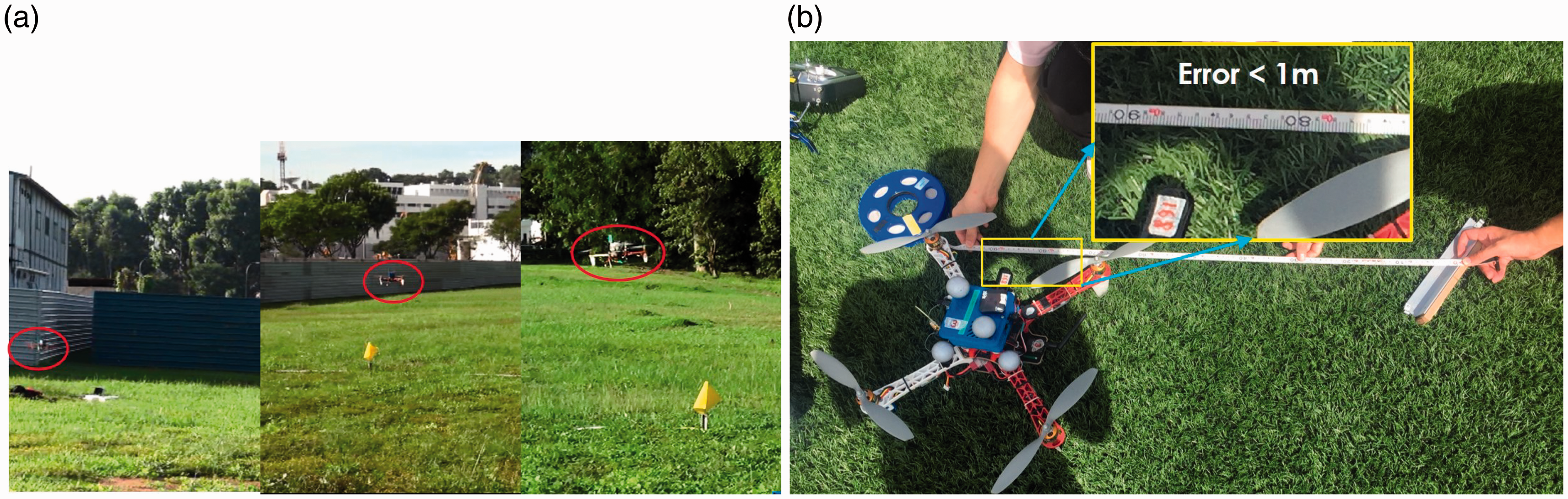
Test environment.

To evaluate the active RL Algorithm 2, flight tests for two UAVs were carried out first as shown in Figure 10, where the moving UAV and the beacon are, respectively, circled in yellow and red. UWB modules were installed on both quadcopters, with one of them placed on the ground as the static beacon. Ten different starting (launching) points were chosen for ten different vectors ${\mathrm{OP}}_0$ . The norms of these vectors were randomly generated from 20 through 50 m, with the corresponding bearings in NE frame from 15° through 95°. The ground truth of the starting points was determined by measuring distance and bearing, respectively. During the experiment, the moving UAV will first take off from the starting point, then fly along the nonlinear and piecewise linear paths as in the simulation before landing. The vector connecting the static beacon and the landing point can be measured similarly as in the case of launching points. In addition, flight experiments for three UAVs were conducted to further corroborate the effectiveness of our proposed RL method, where two UAVs moved simultaneously and one UAV hovered in the sky.

UWB based RL workflow

Figure 11(a) illustrates the workflow of the UWB-based RL system. The UWB module on a hovering quadcopter actively sends ranging requests to neighboring UAVs for distance measurement and communication based on the two-way time of flight ranging method described in Guo et al. ²⁵ Once a distance is obtained by UAV2 and UAV3, it will be calibrated by linear regression where the calibration parameters are determined by a series of experiments in different environments. ²⁵ This calibrated range then goes through the outlier detection before it is stored in the database. To reduce the computation and avoid excessive repetition of similar data, only selected distance measurements and neighbor’s information are recorded and stored. Note that RL initialization algorithm is executed first and its output serves as the initial state estimate for EKF. The follow-up localization is sustained by EKF in a recursive way. Finally, the RL estimate update will be fed into the flight controller for quadcopter navigation as depicted in Figure 11(b).

Figure 11.

System structure. (a) UWB-based relative localization workflow, (b) Diagram of flight control workflow.

Evaluation

Flight tests for two UAVs

Tables 1 and 2 show the absolute estimation error on each direction, respectively, at the launching and landing points for 10 tests. The flight trajectories are shown in Figure 12(b), where each test includes a 1.5 m × 1.5 m nonlinear path (red, phase I), a 6 m linear path (green, phase II) and landing path (blue). Note that the green curves tend to maximize the ranging span relative to the static quadcopter for reducing RL errors as mentioned in Error analysis section. The corresponding ground truth and estimate are also illustrated in Figure 12(a), with circles denoting the error bound of 1 m and 1.5 m, respectively, around the launching and landing points. As can be seen from the tables and Figure 12(a), most of the estimates at the launching points fall within the error bound of 1 m, with the biggest one no larger than 1.5 m. The estimates at the landing points degrade a little, but most still fall within the error bound of 1.5 m. Such a performance is acceptable if we consider that the landing occurs after 12 m of movement, and inevitably the undesirable drift during landing leads to a deviation from each RL estimate. The linearization in EKF may also contribute to the increased error. Nonetheless, a better initial estimate tends to improve the convergence of EKF. ²⁶

Table 1.

Absolute estimation error at launching points.

Test	Range (m)	Angle (°)	$\left|x\right|$ Error (m)	$\left|y\right|$ Error (m)
1	20	24.5	0.267	0.920
2	24	15.5	0.096	1.039
3	27	94.2	0.045	1.187
4	30	51.5	0.498	1.338
5	34	87.5	0.632	0.210
6	37	42.5	0.150	0.858
7	40	78.5	0.755	0.662
8	45	33.5	1.166	0.951
9	47	69.5	0.690	1.106
10	50	60.5	0.103	0.023
		Mean	0.440	0.830

Table 2.

Absolute estimation error at landing points.

Test	Range (m)	Angle (°)	$\left|x\right|$ Error (m)	$\left|y\right|$ Error (m)
1	20	40.2	1.138	1.779
2	24	31.7	1.0	1.062
3	27	108.9	1.417	1.294
4	30	63.7	0.02	0.967
5	34	97.6	2.30	0.355
6	37	51.6	1.174	0.798
7	40	88.0	0.612	0.476
8	45	42.5	1.192	1.094
9	47	76.2	0.186	0.676
10	50	70.3	0.822	0.929
		Mean	0.986	0.943

Figure 12.

Variation of estimation error and flight trajectories. (a) Comparison of relative position estimate and ground truth, (b) Trajectories of 10 flight tests.

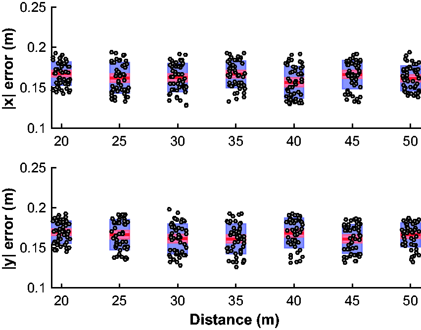
We also examine the variation of the estimation error of the starting point during the whole test, as shown in Figure 13. Note that totally seven different parts of path are involved in the whole duration of RL, corresponding to seven different estimates. From Figure 13, we observe that the error keeps decreasing with the increasing traveling distance, and the ranging along the piecewise linear path drastically reduces the error of the initial estimation. Such a result demonstrates the efficacy of reducing error by enlarging the ranging span as revealed in Theorem 4.1. On the other hand, the decrease of error after each change of heading suggests the necessity of changing heading. We also notice that after some steps the estimation error tends to stabilize, implying that the increase of ranging span is no longer able to counter the displacement error. It would be interesting to explore the relationship when the displacement error increases the estimation error would increase.

Figure 13.

Variation of estimation error at the launching point. (a) |x| error, (b) |y| error.

Flight tests for three UAVs

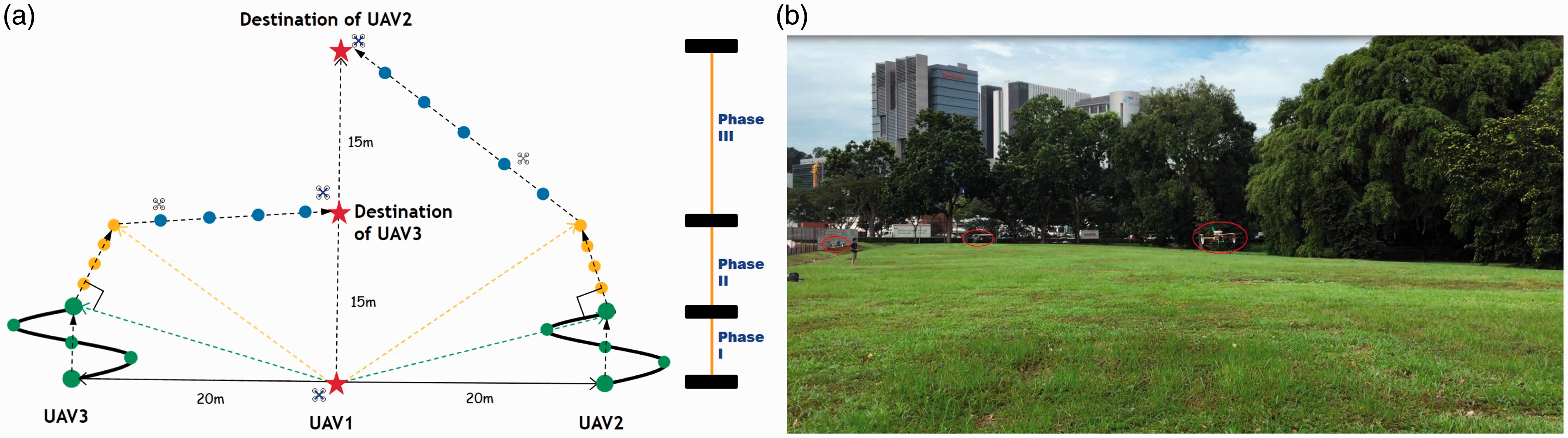
To further validate the performance of the proposed RL method, flight tests of three UAVs were conducted at Dover in Singapore with an area of 30 m × 40 m (Figure 15(b)). First, to support RL estimation among three UAVs, we had to design a new UWB ranging and communication topology, which is different from that utilized for two UAVs. Without clock synchronization among UWB modules, a master-slave ranging mode is adopted to avoid sensing conflicts as shown in Figure 14. Specifically, in our RL context, the module installed on the UAV1 (denoted as M) will actively send its ranging request and odometry data to the module on UAV2 and UAV3 (denoted as S, assume that they are equivalent). The responder module (UAV2 or UAV3) will automatically respond to the ranging request it receives from UAV1 and at almost the same time, collect the ranging and odometry data, which has been synchronized by the master node one time slot afore.

Figure 14.

Ranging topology in master-slave pattern.

Figure 15.

Fight demo of three UAVs at Dover. (a) Demo scenario at Dover, (b) Flight video shot of 3 UAVs at Dover.

Figure 16.

Flight performance based on RL estimate. (a) Performance of the relative localization for 3 UAV's (b) Accuracy of the relative localization measured after landing.

Subsequently, the UWB module M installed on UAV1 transmits and receives ranging command signal as well as odometry information from UAV3 at $M_{t_2}^{T_x}$ and $M_{t_3}^{R_x}$ , respectively. And the distance to UAV3 can be achieved by $(M_{t_3}^{R_x}-M_{t_2}^{T_x}-{\delta }_S)\times c/2$ . UAV1 switches ranging ID of UAV2 and UAV3 alternately in each loop at a fixed ranging rate of 20 Hz.

Since the reference of our relative position estimate can be any customized coordinates, a baseline herein, which is parallel to a ditch nearby with 233° relative to the north, was first selected for calibrating the ground truth. UAV2 and UAV3 are desired to navigate to their destinations based on the gap between the preconfigured destinations and their real-time RL estimates to UAV1. In this test, the destination points relative to UAV1 were set preliminarily based on the method in “Methodology” section and marked by yellow flags as shown in Figure 16(a). UAVs will hover over their destination points once they reach them. Such performance is able to demonstrate the practicability of our UWB-based RL and the accuracy of landing reveals the applicability of the proposed RL method. The following gives a detailed description on the flight experiment.

Initially, UAV1 was set in the middle of UAV2 and UAV3 with 20 m interval as shown in Figure 15(a). Once all of the UAVs were powered on, UAV1 started automatically to range and communicate with UAV2 and UAV3. After taking off, UAV1 hovered over its launching point while UAV2 and UAV3 flied along a preset non-linear trajectory for collecting distance data and calculating the initial relative position, namely phase I. The RL estimates were improved when UAV2 and UAV3 flied along a piecewise linear path during phase II. Based on the difference between the on-line RL estimates and their preset destinations, in phase III, UAV2 and UAV3 navigated directly to their desired target positions (the red stars in Figure 15(a)). The flight video shot is shown in Figure 15(b). Finally, all of these three UAVs hovered over their destination as seen in Figure 16(a) with the position error less than 1 m (Figure 16(b)). More details concerning the trajectories of three UAVs are depicted in Figure 17 where UAV2 and UAV3 eventually hovered over their relative targets to UAV1, at (0,30) and (0,15), respectively, and the RL estimation errors both fell within the 1 m error bound (cyan circle). Note that the RL error was measured after UAVs landed and in fact there always existed an inevitable drift during landing (e.g. avoiding to land on the marker, wind disturbance, near-ground effect, and control accuracy). Such drift would cause an undesirable deviation from each RL estimate. Despite this, a RL accuracy with less than 1 m can be acceptable when considering the maximum inter-UAV distance reaches 30 m in this scenario. ^a

Figure 17.

Flight paths of three UAVs.

Conclusion and future work

In this article, we studied the UWB based RL problem for an UAV team. An active RL problem of a moving UAV with respect to a static UAV under motion constraint was introduced first. Specifically, the UAV is only allowed to move by a small distance D and we aim to find a ranging path to reduce the RL error as much as possible. We considered the problem under the assumption of noise-free self-displacements, and reformulated it as an optimal sensor placement under constraint. A lower bound of estimation error was obtained in terms of D and the sample size n, and it was found that one only needs to enlarge the ranging span and increase the number of rangings to reduce the error. In this light, we designed an active RL algorithm to enlarge the ranging span within the distance D, and applied the EKF to account for the noise in the displacement measurements. Simulations and experiments were conducted to validate the algorithm.

Second, we extend the EKF based RL method to a dynamic UAV group where the beacon UAV starts to move and the RL estimate from the first stage is fed into the proposed cooperative RL algorithm for initialization. To validate the accuracy of the cooperative RL estimate during UAVs’ simultaneous flight, a simulation without control laws was conducted and the error bound falls within 0.8 m on average.

In the future, we shall extend the current result to 3D case under more general constraint, and an UWB based formation flight will be explored and tested.