Multidisciplinary design optimization of the flapping wing system for forward flight

Abstract

The success of a flapping wing air vehicle flight is strongly related to the flapping motion and wing structure. Various disciplines should be considered for analysis and design of the flapping wing system. A design process for a flapping wing system is defined by using multidisciplinary design optimization. Unsteady aeroelastic analysis is employed as the system analysis. From the results of the aeroelastic analysis, the deformation of the wing is transmitted to the fluid discipline and the dynamic pressure is conveyed to the structural discipline. In the fluid discipline, a kinematic optimization problem is solved to maximize the time-averaged thrust coefficient and the propulsive efficiency simultaneously. In the structural discipline, nonlinear dynamic topology optimization is performed to find the distribution of reinforcement by using the equivalent static loads method for nonlinear static response structural optimization. The defined design process is applied to a flapping wing air vehicle model and the flapping wing air vehicle model is fabricated based on the optimization results.

Introduction

Flapping wing systems of birds, insects, and fish have drawn strong attention from the engineering community because they could offer extensive potential applicability to numerous small-scale aerial vehicles and propulsive devices/mechanisms. Flapping wing micro air vehicles (FWMAVs) imitate the flapping wing system for a more efficient flight. The FWMAVs have a dimension on the order of 15 cm and the flight speed of approximately 10 m/s. The unsteady aerodynamic performance is related to the flow characteristics at the low Reynolds number. Numerous research groups are actively studying the design of the FWMAV. The flapping performance, such as the thrust coefficient and propulsive efficient, is strongly related to the flapping wing system which consists of the flapping motion and wing structure. Thus, optimization of the flapping motion and wing structure is desired for the best flapping performance.

Many experimental and computational researches have been carried out to maximize the flapping performance. Anderson et al. ¹ showed that a harmonically oscillating foil could have very high propulsive efficiency, as high as 87%, under specific combinations of the flapping kinematics by water tunnel experiments. Pesavento and Wang ² found that the optimized flapping wing motions could save up to 27% of the aerodynamic power required by an optimal steady flight. In 2005, Tuncer and Kaya ³ utilized the steepest ascent search algorithm to maximize the thrust and/or propulsive efficiency of single flapping airfoils. In 2007, Kaya and Tuncer ⁴ obtained the optimal flapping kinematics to improve the maximum thrust and propulsive efficiency by using a nonuniform rational B-spline, and a gradient-based search algorithm was employed to find the optimum. In 2009, Kaya et al. ⁵ extended their optimization scheme to a biplane configuration. In 2011, Choi et al. ⁶ performed kinematic optimization for an efficient flight, and the results were applied to the wing structure for dynamic response topology optimization. In 2013, Choi et al. ⁷ investigated various flapping motions for maneuverability and sustainability flights.

Most past optimization researches considered the wing as a rigid body for kinematic optimization. Recently, some optimization studies consider the deformation of the wing structure to evaluate the aerodynamic performance.^8,9 However, optimization researches on flapping kinematics and the wing structure are rare for a practical flapping wing design. The research results from biologists and physicists indicate that the flexibility of the flapping wing has unnegligible effects on its performance, such as the thrust and propulsive efficiency.^10–13 Especially in the case of insect-inspired FWMAVs, the flexible wing is constructed using a combination of materials (carbon, nylon, and mylar) for the veins and latex membrane. The flexibility significantly depends on the vein distribution. In order to consider the flexibility, aeroelastic analysis is required to predict the response of a flapping wing system precisely. It is quite difficult to directly use the high-fidelity aeroelastic analysis in the optimization process due to the high computational cost. Many researches use the simple model that has a small number of elements for unsteady aeroelastic analysis. Thus, an analysis with moderate fidelity is generally carried out.

Many studies on optimization have been conducted considering aeroelasticity. Stewart et al. ¹⁴ performed shape optimization of the wings in forward flight. The aeroelastic model tightly coupled a structural plate finite element model with an aerodynamic model for the unsteady vortex lattice method (UVLM), and a gradient-based optimization was used to maximize the average thrust. Stanford and Beran ¹⁵ explored gradient-based aeroelastic optimization based on the complex interaction between fluid and structure for optimal performance. Ghommema et al. ¹⁶ optimized the shape of flapping wings in forward flight. The analysis was performed by combining a gradient-based optimizer with the UVLM. Several parameters affecting the flight performance were described. Stewart et al. ¹⁷ performed shape optimization of a plate-like flapping wing. The aeroelastic system was analyzed by using an unsteady vortex lattice aerodynamic model with a plate finite element model. Two multiobjective optimization formulations were defined for the wing shape and structure. The results showed that the added wing deformation had benefits for the thrust and more power is required for the flapping motion. It is noted that the studies on aeroelastic optimization generally concentrate on structural optimization of a plate-like flapping wing and do not solve the optimization problem using aerodynamic analysis. Moreover, moderate-fidelity computational tools were used and a nonlinear shell model was coupled to an UVLM to reduce the cost of aeroelastic analysis. However, UVLM cannot consider viscous effects such as a flow separation, transition, reattachment, etc. ¹⁸ It is noted that high-fidelity Navier–Stokes flow solvers are typically quite expensive. Most studies have a few design variables for a response surface-based surrogate optimization.^19,20

Some researchers have studied the reinforcement and planform of the flapping wing. Ansari et al. ²¹ developed an aerodynamic model and used the model for the analysis of 13 planforms. The planforms had different dimensions according to the area and aspect ratio. Ansari et al. ²² described the wing planform as a set of blade elements and used the parameterization technique which was limited and only allowed designs that were symmetric with respect to the midchord. Stewart et al. ²³ developed a novel parameterization technique and it would allow for planform designs that were not symmetric about the midchord. The planform of a rigid flapping wing was optimized for the forward and hovering flights. Topology optimization is carried out to keep certain rigidity of the flapping wing with a specific mass. It is noted that there are not many studies on the topology optimization of the flapping wing. The topology of stiff battens within a membrane wing has been studied for both fixed wings ²⁴ as well as flapping wings.^25,26 The stiffness of a membrane wing can also be varied by changing the applied prestress. The structural stiffness distribution can be controlled by the thickness of the wing for a plate-like wing.

Generally, computational fluid dynamic (CFD) analysis or experiments are utilized for kinematic optimization of the flapping motion while the structure is assumed to be rigid. However, the flexibility of the structure has a significant effect on kinematic and structural optimizations. Recently, structural optimization of a flapping wing structure is being actively studied to consider the flexibility of the flapping wing. A simple structure such as a plate-like flapping wing is usually used for structural optimization and aeroelastic analysis with UVLM is used to consider the flexibility. It is well known that UVLM cannot consider the viscous effects. However, the viscosity effects are crucial in the characteristics of the flapping. In order to consider the viscosity effect, aeroelastic analysis is required based on the high-fidelity Navier–Stokes flow solvers. It is generally quite expensive. This research considers various disciplines such as CFD analysis, structural analysis, high-fidelity aeroelastic analysis, and structural optimization. Aeroelastic analysis is required to identify the characteristics of the flapping wing structure and the analysis results should be systematically incorporated in the design process. When various disciplines are involved in an optimization process of a complicated system, a technique of multidisciplinary design optimization (MDO) should be utilized. Thus, an effective design process is needed for MDO of the flapping wing system.

In this research, a design process for a flapping wing system is defined by using an MDO method called multidisciplinary design optimization based on independent subspaces (MDOIS). ²⁸ In MDOIS, each discipline is independently solved and the coupled aspects are considered in the system analysis. Three-dimensional unsteady aeroelastic analysis is employed as the system analysis. The results of the system analysis are transmitted to the two disciplines: the wing deformation is transferred to the aerodynamic discipline and the dynamic pressure is provided to the structural discipline. Therefore, it can reduce the cost of high-fidelity unsteady aeroelastic analysis. In the aerodynamic discipline, an optimization problem is solved to maximize the time average thrust coefficient and the propulsive efficiency. The optimization process is carried out based on a design of experiment methodology and a well-defined surrogate model. The surrogate model is made from the results of two-dimensional unsteady aerodynamic analysis. The response surface method (RSM) ²⁹ is employed to establish the surrogate model and a genetic algorithm ³⁰ is used for the multiobjective function problem.

In the structural discipline, nonlinear dynamic response topology optimization is carried out to find the reinforcement distribution. Nonlinear dynamic response topology optimization is conducted by using the equivalent static loads method for nonlinear static response structural optimization (ESLSO). ESLSO has been extensively used for size, shape, and topology optimizations.^31–34 The objective function to minimize is the strain energy and the design variables are the intermediate density variables. The defined design process is applied to an initial flapping wing air vehicle (FWAV) model which is fabricated from experience and previous researches. The optimized flapping motion (kinematics) and reinforcement distribution are obtained from the design process. Finally, the optimized FWAV model is fabricated according to the optimization results.

The design process is applied to solve the problem by integrating various software systems. ADINA ³⁵ is used for unsteady aeroelastic analysis and FLUENT ³⁶ is used for unsteady aerodynamic analysis. Nonlinear dynamic analysis is performed using LS-DYNA. ³⁷ NASTRAN ³⁸ is used for the computation of the linear stiffness matrix and the calculation of the equivalent static loads (ESLs). OptiStruct ³⁹ is used for topology optimization and PIAnO ⁴⁰ is used for optimization using RSM. An in-house C++ program ⁴¹ is coded to integrate the systems.

Design process using MDO

This research starts from an initial FWAV as illustrated in Figure 1. The flapping motion along the vertical stroke plane is defined by a sinusoidal plunging motion. A design process is defined to optimize the flapping wing system of the model by using MDO.

Figure 1.

Initial model of the flapping wing air vehicle.

FWAV

As illustrated in Figure 1, an FWAV is fabricated based on the previously developed FWAV.^42,43 The components, which consist of a motor, a receiver, a speed controller, a battery, and gears, are selected from inexpensive commercially available components. The wing of the FWAV is comprised of the reinforcement and the membrane structure. A 1 mm thickness carbon rod is used for the reinforcement of the wing and a 0.02 mm mylar is used for the membrane structure. The tail wing, which consists of the vertical and the horizontal wings, is fabricated for the change of the flight direction. Table 1 shows the specifications of the model. The flapping motion causes wing deformation during the flight and the deformation significantly depends on the distribution of the reinforcement and flapping kinematics. Thus, the design of the wing structure should consider the relationship between the deformation and reinforcement.

Table 1.

Specifications of the initial flapping wing air vehicle.

Wing span	34 cm	Wing area	204 cm2
Weight	21 g	Maximum frequency	15 Hz
Fuselage length	26 cm	Upstroke angle	38°
Gear ratio	20:1 reduction	Downstroke angle	−5°

The three-dimensional flapping kinematics can be mathematically formulated by introducing many independent model parameters such as the frequency, the flapping amplitude, and the mean position. The flapping motion is implemented by the movement of the leading edge. The movement of the leading edge is assumed to be harmonic as illustrated in Figure 2. The flapping motion can be described as follows

$\theta (t)=\alpha +{\theta }_0\cos (\omega t)$

(1)

where $\theta (t)$ stands for the flapping motion, α is the mean position, ${\theta }_0$ is the flapping amplitude, ω is the angular frequency in rad/s, and t is the time.

Figure 2.

Flapping motion of the FWAV.

In classical aerodynamics, the Reynolds number ( $\mathrm{Re}$ ) is defined as follows

$\mathrm{Re}=\rho \mathrm{uc}/\mu$

(2)

where ρ is the fluid density, u is the far-field velocity, c is the chord length, and μ is the fluid dynamic viscosity. The drag coefficient C_D and the lift coefficient C_L are defined as

$C_D=\frac{F_x}{0.5\rho u^{2}S}$

(3)

$C_L=\frac{F_y}{0.5\rho u^{2}S}$

(4)

where F_x and F_y are the components of the resulting aerodynamics force along horizontal (parallel with u direction) and vertical (normal to u direction) directions, respectively. S is the reference area and equals to c in a two-dimensional problem. The time-averaged thrust coefficient ${\overline{C}}_T$ and the power input coefficient ${\overline{C}}_P$ in one flapping cycle can be calculated by equations (5) and (6). Correspondingly, the propulsive efficiency η is defined in equation (7)

${\overline{C}}_T=-{\overline{C}}_D=-\frac{1}{T}{\int }_t^{t+T}{C}_D(t)\text{d}t$

(5)

${\overline{C}}_P=\frac{1}{T}{\int }_t^{t+T}{C}_L(t)\stackrel{·}{y}(t)\text{d}t$

(6)

$\eta =\frac{{\overline{C}}_{T}u}{{\overline{C}}_P}$

(7)

where T is the period in seconds with $T=1/f$ and $\stackrel{·}{y}(t)$ is the first-order time derivative of $y(t)$ . In this research, the section of the wing moves up and down and $y(t)$ is the location of a point in the wing section. The propulsive efficiency is the ratio of the power for generation of the thrust to the power input required to keep the flapping motion. The power input coefficient accounts for the rate of the average work required to maintain the flapping motion. In this research, only the aerodynamic power is considered. ³

Description of the design process

As mentioned earlier, the flapping wing system is optimized using an MDO method called MDOIS. ²⁸ Various techniques for MDO are introduced and the features, advantages, and disadvantages are described in Martins et al. ⁴⁴ MDOIS is a practical MDO method that can be applied to practical engineering problems.^45,46 It is a single level MDO method, which has a system analysis and decomposed disciplines as illustrated in Figure 3. Disciplines are coupled only in the analysis process. An independent optimization problem is defined for each discipline. The coupling aspects are evaluated in the system analysis and transferred to each discipline. The optimization problem of each discipline is solved independently. Therefore, the computational cost is reduced significantly because the system analysis is not directly used in optimization. When each discipline changes its design variables through optimization, the results will affect other disciplines. It is evaluated from the system analysis of the next cycle. If all the design variables are unchanged in optimization, the process terminates.

Figure 3.

Flowchart of MDOIS.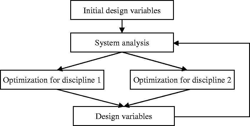

The aerodynamic performance of the FWMAV is mainly affected by the flapping motion and wing structure. Kinematic optimization and structural optimization can be defined in each discipline. The flapping kinematics causes wing deformation, and the deformation significantly affects the aerodynamic performance. Thus, the design of the flapping wing system should consider the relationship between the flapping motion and wing structure. Three-dimensional unsteady aeroelastic analysis is utilized for this in system analysis because the pressures on the three-dimensional flapping wing are required in structural design. It is important to reduce the number of the costly system analyses.

Optimization of the flapping wing system can be divided into kinematic optimization and structural optimization. In kinematic optimization, the objective function to maximize is the time average thrust coefficient and the propulsive efficiency. The design variables are the flapping kinematic parameters. In structural optimization, the objective function to be minimized is the strain energy and the artificial material density in every finite element of the structure is treated as the design variable for topology optimization. The design variable has a certain value between 0 and 1. If the design variable is close to 0, the corresponding element is considered empty.

The two optimizations are physically separate so they can be carried out independently. In other words, only local design variables are used for each discipline and a discipline has its own objective function and constraints. Therefore, MDOIS is suitable to use in this case.

A design process is defined by considering the flow of MDOIS and the process is presented in Figure 4. The flapping wing system is decomposed into two disciplines—aerodynamic discipline and structural discipline. The deformed shape and pressure distribution are determined in system analysis and transmitted to each discipline where they are used as constant parameters. After that, an independent optimization process is carried out in each discipline. The optimum solution from each discipline is transmitted again to the system analysis. This procedure makes one cycle and the process continues until the convergence criterion is satisfied.

Figure 4.

Design process for the flapping wing system.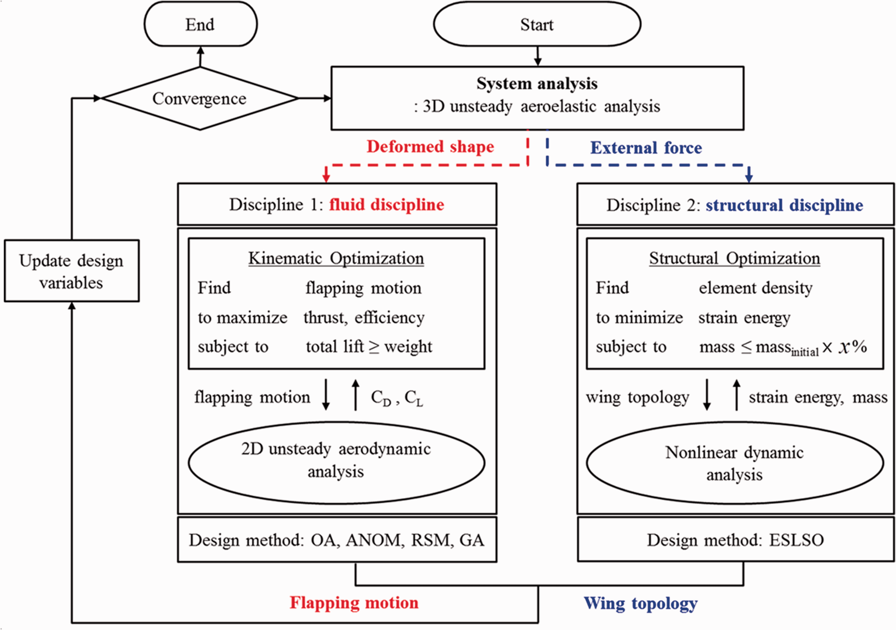

Two types of analyses are required for the two disciplines. They are unsteady aerodynamic analysis in the aerodynamic discipline and nonlinear dynamic analysis in the structural discipline. From the system analysis, the deformed shapes of the wing structure are transferred to the aerodynamic discipline because the time-dependent shape of the airfoil is important for the calculation of the aerodynamic performance. In the aerodynamic discipline, kinematic optimization is carried out to maximize the aerodynamic performance such as the time-averaged thrust coefficient and propulsive efficiency. Two-dimensional unsteady aerodynamic analysis is conducted for kinematic optimization because three-dimensional unsteady aerodynamic analysis is extremely expensive in the optimization process. Obviously, two-dimensional unsteady aerodynamic analysis cannot predict the three-dimensional effects (e.g. the wing tip vortices and the spanwise flows). The results of two-dimensional analysis are not as accurate as those of three-dimensional analysis. However, we expect that the trends of two-dimensional kinematic optimization are acceptable approximations for three-dimensional unsteady aerodynamic analysis. ⁴⁷ The two-dimensional unsteady aerodynamic analysis uses the cross-section wing at the halfway point in the spanwise direction.

For structural design, the pressure distribution is required in the time domain because the flapping motion is transient. The time-dependent pressures (dynamic pressure) on the flapping wing are transferred to the structural discipline from the system analysis. In structural optimization, the dynamic pressure is used as the external loads for nonlinear dynamic analysis of the flapping wing structure. The flapping wing structure should pursue a light mass and sustain the aerodynamic force during the flapping motion. The objective of the structural optimization is defined based on the results of previous research. ⁶ Therefore, topology optimization is performed to find the distribution of reinforcement with a specific mass to maximize the stiffness of the wing structure. Nonlinear dynamic response topology optimization is conducted by using the ESLSO. In this research, the defined design process is applied to the model of Figure 1 that is the initial baseline design for the optimization process.

System analysis

The flexible wing structure has a strong interaction between the deformation and the surrounding airflow. The mesh system is fixed on a certain coordinate system in a general analysis of fluid. That is, the Eulerian description of the fluid flow is used for fluid analysis. However, the Eulerian description is no longer applicable in aeroelastic analysis because any part of the computational domain deforms. Structures are usually described by the Lagrangian formulation. Therefore, finite element analysis based on the arbitrary Lagrangian–Eulerian (ALE) method was developed and successfully applied to problems such as artificial heart pulsation and flapping flight. ⁴⁸ In this research, ADINA ³⁵ is employed to simulate unsteady aeroelastic analysis. The direct fluid structure interaction (FSI) coupling method is used to solve the coupling between the fluid and structure models. In this method, the time-dependent Navier–Stokes equations based on the ALE method are utilized assuming an incompressible laminar flow. In the research of the flapping wing, an important point is that the researchers of a fluid structural interaction problem frequently do not know how high a Reynolds number flow will be encountered and what turbulence model should be used. Hence, the problem is frequently best solved first by assuming laminar conditions. The fluid and structure governing equations based on the ALE method are merged into a single matrix equation by the finite element method. ⁴⁸ After that, the matrix is linearized and solved using an iterative algorithm such as the Newton–Raphson method. The direct FSI coupling method offers great robustness when solving a very difficult FSI problem, for example a flapping wing model with large deformation.

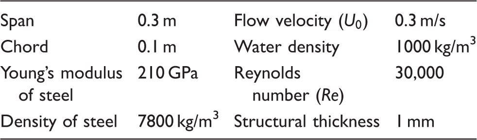
A water tunnel study was performed for the effect of spanwise flexibility on the thrust, lift, and propulsive efficiency of a rectangular wing oscillating in a pure heave by Heathcote et al. ¹¹ To validate the accuracy of the system analysis, the simulation results are compared with the results of Heathcote et al. ¹¹ Thus, the accuracy of system analysis is validated through the comparison. A schematic of the experimental setup is illustrated in Figure 5 where c is the chord length. A wing of 0.3 m span and 0.1 m chord is constructed. The leading edge at the wing root is actuated by a prescribed sinusoidal plunging motion. The motion can be described as follows

$y(t)=h\mathbf{cos}(\omega t)$

(8)

where $h$ is 0.175 and ω is 5.46. The analysis condition is shown in Table 2. The fluid model, which is illustrated in Figure 6, is employed to compute the flow field. The fluid domain, which is composed of tetrahedron elements, is the remeshing zone. The wing structure is located at the center of the fluid domain. The structure model is composed of solid elements as illustrated in Figure 7. The root of the wing is fixed to a point by rigid elements. Simulation is executed in 10 plunging periods. The one plunging period is divided into 58 and 115 points, respectively. This means the nondimensional time step. The overall wing thrust coefficient and the normalizing quantity of the tip displacement response are compared with the experimentally measured data of Heathcote et al. ¹¹ The two results are quite close as illustrated in Figure 8. The tip displacement in Figure 8(b) is a normalized value by the plunging amplitude of the wing root. From the validation, the simulation is employed for system analysis.

Figure 5.

Schematic of the spanwise flexible wing heaving periodically. ¹¹

Table 2.

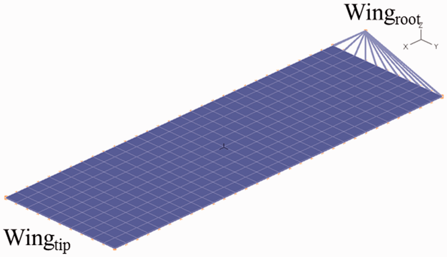
Analysis conditions for verification of aeroelastic analysis.

Span	0.3 m	Flow velocity (U0)	0.3 m/s
Chord	0.1 m	Water density	1000 kg/m3
Young’s modulus of steel	210 GPa	Reynolds number (Re)	30,000
Density of steel	7800 kg/m3	Structural thickness	1 mm

Figure 6.

Fluid model for the rectangular wing.

Figure 7.

Solid finite element model of the thin rectangular steel.

Figure 8.

Time histories of thrust coefficient and tip displacement: (a) thrust coefficient and (b) tip displacement.

In this research, the fluid and structure models are made for aeroelastic analysis of the initial model in Figure 1. Figure 9 presents the fluid model and the analysis conditions are shown in Table 3. The fluid model has about 70,000 tetrahedron elements. The elements near the wing structure are dense. The flapping frequency is assumed to be 11 Hz. Figure 10 illustrates the finite element model for the structure model and the material properties are shown in Table 4. The finite element model has two shell element layers for structural optimization and each layer has 6760 shell elements. Two shell element layers are divided into the design domain (carbon) and the nondesign domain (mylar) for topology optimization. The design domain is the inner layer of the shell elements without the leading edge and rigid connection points. Common nodes are used for the design and nondesign domains. The pressure of the nondesign domain is transferred to the design domain through the common nodes. Therefore, the two domains should have the same degrees of freedom, and the two domains are modeled by shell elements. Actually, the nondesign domain should be modeled by membrane elements that do not have bending degrees of freedom, so this modeling process can generate some numerical error. The pressures are always applied on the nondesign domain and the nondesign domain is supported by the design domain. Therefore, the shell element layer of the design domain is changed during the topology optimization process except for the nondesign domain. The boundary condition is imposed on the root of the leading edge. All the degrees of freedom in six directions are fixed. The cross-section of the wing structure is assumed to be a thin plate. Unsteady aeroelastic analysis is carried out in 10 periods with 1820 time steps in one flapping period to facilitate regeneration of the elements because the wing deformation is large. In the first cycle, the analysis conditions are $\alpha =15$ , ${\theta }_0=20$ , and $\beta =0$ for unsteady aeroelastic analysis because the initial model of FWAV is fabricated according to these values.

Figure 9.

Fluid model of the wing for aeroelastic analysis.

Table 3.

Properties of the fluid model for aeroelastic analysis.

Condition	Value
Flow velocity	3 m/s
Air density	1.225 kg/m3
Air viscosity	1.7894 ×  ${10}^{-5}$  kg/(m s)
Reynolds number	24,645

Figure 10.

Finite element model of the wing for aeroelastic analysis.

Table 4.

Material properties of the structure model for aeroelastic analysis.

Property	Value
Span/chord	0.17 m/0.12 m
Young’s modulus of carbon	170.3 GPa
Density of carbon	2001.2 kg/m3
Young’s modulus of mylar	3.28 GPa
Density of mylar	1400.6 kg/m3
Carbon thickness	0.5 mm
Mylar thickness	0.1 mm

Kinematic optimization in the aerodynamic discipline

In the aerodynamic discipline, kinematic optimization is carried out by using the deformed shape from the system analysis. The objective function to be maximized is a multiobjective function which is composed of the thrust coefficient and the propulsive efficiency. Unsteady aerodynamic analysis is required to evaluate the objective function. It is difficult to use a gradient-based optimization algorithm because the sensitivity analysis with unsteady aerodynamic analysis is extremely expensive. Moreover, two-dimensional unsteady aerodynamic analysis is utilized because three-dimensional unsteady aerodynamic analysis is quite expensive. The relationship of the design variables between the three-dimensional wing and the two-dimensional airfoil is defined as follows: First, the three-dimensional wing is flapped based on the design variables of kinematic optimization in the unsteady aeroelastic analysis. Second, the two-dimensional airfoil is assumed by the cross-section at the halfway point in the spanwise direction. The deformation of the section is obtained. In the same cycle of the design process, the deformations of the airfoil are assumed to be the same. The position of the rigid airfoil is changed by the design variables. Finally, the x and y positions of the two-dimensional airfoil is calculated in addition to the position of the rigid motion and the deformation.

In this research, the design process in the aerodynamic discipline is defined for the kinematic optimization as illustrated in Figure 11. First, the design variables and their levels are determined. An orthogonal array (OA) ²⁹ is selected and the objective function is evaluated for each row of the OA by unsteady aerodynamic analysis. In the matrix experiment, the deformed shape of all rows is assumed to be the same because the system analysis provides only one result. Therefore, the matrix experiment is conducted by a modified shape from the deformed shape of the system analysis. The modification is made according to the design variables. A candidate optimum solution (Solution 1) is obtained from the OA. That is, Solution 1 is the best one out of the rows of the OA. After that, analysis of mean (ANOM) ²⁹ is performed by using a one-way table. Another candidate optimum solution (Solution 2) is obtained from the ANOM and a confirmation experiment is carried out. The detailed process is explained in Park. ²⁹ In the continuous design, the other candidate optimum solution (Solution 3) is obtained by using a surrogate model. The surrogate model is made by the candidate points of the OA. A genetic algorithm is utilized to find the optimum of the surrogate model. Since the solution is from an approximate surrogate model, a confirmation experiment is carried out as well. These three solutions are compared and an appropriate one is selected according to the design purpose.

Figure 11.

Design process for kinematic optimization.

Two-dimensional unsteady aerodynamic analysis

Unsteady flow fields around the moving wings with the deformed shape are simulated by the commercial CFD solver FLUENT. ³⁶ The time-dependent Navier–Stokes equations are solved using the finite volume method, assuming incompressible laminar flow. The mass and momentum equations are solved in a fixed inertial reference frame incorporating a dynamic mesh.

The mesh that is illustrated schematically in Figure 12 is employed to compute the flow field. The computational domain is the remeshing zone which consists of the unstructured triangular mesh. The airfoil is located at the center of the computational domain and the no-slip wall boundary condition is applied. The spatial scale of the domain and corresponding boundary condition are also presented in Figure 12. The airfoil moves based on the coordinate of the deformed shape according to the time. The C-type mesh structure in the very close neighborhood of the airfoil is illustrated in Figure 13, and the grid size is 201 × 101 nodes (201 along every single airfoil surface and 101 in the vertical direction) with the thickness of the first layer grid around the airfoil equal to 0.0002c. The mesh is generated by ICEM CFD. ⁴⁹

Figure 12.

Mesh topology with boundary conditions.

Figure 13.

Grid very close to the airfoil.

Application of the deformed wing shape

The coordinates of the deformed wing shape are obtained with respect to the time from the system analysis. The reason is that the coordinates should be considered according to the time in two-dimensional unsteady aerodynamic analysis. Therefore, an analysis method is required for the deformed wing shape. Garvin et al. ⁵⁰ performed unsteady CFDs simulation for the fish motion. The x and y coordinates of the moving body were taken from a video and utilized in the CFD simulation to capture the fish motion according to the time. The user-defined function (UDF) and dynamic mesh module in the commercial software system FLUENT ³⁶ were used in the simulation. The dynamic meshing option in FLUENT can accommodate the mesh points of a moving body. The mesh points of the fish body move with a prescribed velocity given by a customized code. The code is written in the C language.

In this research, the same method is utilized for the simulation of a deformed wing shape. The application process is shown in Figure 14. First, the x and y positions of the corresponding deformed wing shape are obtained from the aeroelastic analysis (system analysis). Second, the mesh is created based on the initial geometry of the wing section and then unsteady aerodynamic analysis is carried out based on the x and y positions of the deformed wing shape according to the time by using the UDF and dynamic mesh module of FLUENT.

Figure 14.

Overview of coupled aeroelastic analysis and aerodynamic analysis.

In order to validate the accuracy of the present approach, the results of the two-dimensional unsteady aerodynamic analysis are compared with the data of a previous research. ⁵¹ In aeroelastic analysis, the NACA0014 airfoil is used, and it is assumed to be a rigid body because the previous research ⁵¹ used the rigid body model for simulation. The objective of the validation is the verification of the analysis method using the x and y positions of the wing shape according to time. The plunging motion of the airfoil is as follows

$y(t)=\mathrm{hc}\mathbf{cos}(\omega t)$

(9)

where h is 0.4, c is 0.064 m, and ω is 1084.375 rad/s. The analysis conditions are $u=34.7$  m/s and Re = 10,000. The x and y coordinates of the airfoil are obtained from the aeroelastic analysis. Simulations are executed in seven periods with 500 time steps in one plunging period. The coupling between the pressure and the velocity is achieved by means of the SIMPLEC algorithm. ³⁶ Meanwhile, discretization of the pressure and momentum terms is the second-order scheme and the second-order upwind scheme. The time discretization is the first-order implicit scheme, which is a more straightforward method in FLUENT for the dynamic mesh module. The time history of the drag coefficient in one period is illustrated in Figure 15, with the results of Tuncer and Kaya. ⁵¹ These results show a good agreement, even though different mesh schemes are employed in the two studies.

Figure 15.

Validation for unsteady aerodynamic analysis.

Design formulation for kinematic optimization

Thrust is primarily generated by the flapping motion of the initial model because the wings of FWAV flap in a vertical stroke plane. The model should be designed to have maximum thrust and high efficiency. The kinematic optimization problem is formulated as follows

$\text{Find}\alpha ,{\theta }_0,\beta \text{to}\hspace{1em}\text{minimize}f(\alpha ,{\theta }_0,\beta )=(1-b)\frac{{\overline{C}}_T-{\overline{C}}_{T,max}}{{\overline{C}}_{T,min}-{\overline{C}}_{T,max}}\text{subjectto}\mathrm{\hspace{1em}\hspace{1em}\hspace{1em}}+b\frac{\eta -{\eta }_{max}}{{\eta }_{min}-{\eta }_{max}}-{\overline{C}}_T\le 0-\frac{1}{T}{\int }_t^{t+T}{F}_y(t)\text{d}t+\mathrm{weight}\le 05^{\circ }\le \alpha \le {25}^{\circ },{10}^{\circ }\le {\theta }_0\le {30}^{\circ },\mathrm{\hspace{1em}\hspace{1em}\hspace{1em}}{0}^{\circ }\le \beta \le 8^{\circ }$

(10)

where α is the mean position of the flapping motion; ${\theta }_0$ is the flapping amplitude; β is the initial angle of attack; b is the weighting factor; ${\overline{C}}_{T,min}$ and ${\overline{C}}_{T,max}$ are the minimum and the maximum time-averaged thrust coefficients in the design array for constructing the RSM model, respectively; and ${\eta }_{min}$ and ${\eta }_{max}$ are the minimum and the maximum propulsive efficiency in the design array for constructing the RSM model, respectively. The lift force according to time is $F_y(t)$ . The weight in a constraint is a constant of 21 g which is the weight of the initial FWAV model. The design variables are presented in Figure 16. The weighting factor b in the objective function is assumed to be 0.5. It is fixed during the progress of the MDOIS loop. The time-averaged thrust coefficient and the propulsive efficiency are simultaneously maximized because the primary objective of the target model is forward flight.

Figure 16.

Design variables for kinematic optimization of the flapping wing: (a) front view and (b) side view.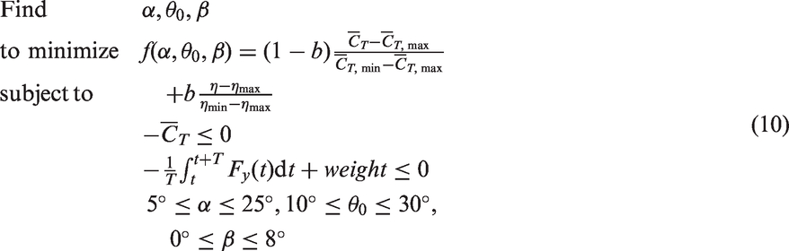

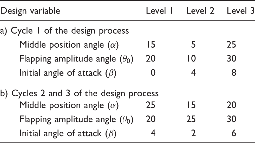
The surrogate model is a versatile and valuable tool for a complex engineering problem. The greatest benefit of the surrogate model would be to save the cost of computational analysis with acceptable approximation accuracy. In this research, the RSM model is employed as the approximation method for the surrogate model, and the OA is used for the cases to make the RSM model. The design spaces are defined very carefully from the initial FWAV model. The OA is an array that easily enables the design of experiments and provides an efficient set of representative parameter combinations. ²⁹ The design variables have three levels and the design array consists of the union of the 18 samples obtained from a classical OA. Conventionally, it is represented by $L_{18}(3^3)$ , where the 18 indicates 18 trials in total, 3 is the number of levels, and 3 for the exponent is the number of design variables. RSM models are constructed to fit the time-averaged thrust coefficient, the propulsive efficiency, and the time-averaged lift force according to the design formulation, respectively. The commercial software PIAnO ⁴⁰ is utilized for the RSM models.

Optimization results of the kinematic optimization

Kinematic optimization is performed according to the design process of Figure 11. The genetic algorithm embedded in PIAnO ⁴⁰ is employed to solve the optimization problems. The maximum generation is set to be 500, and the genetic algorithm is terminated when the tolerance between the current objective function and the previous objective function is smaller than 1.0 × 10⁻⁸. The process is also terminated when the generation reaches 200. Consequently, three candidate optimum solutions are obtained by the design process of Figure 11. The best one is picked as the final solution. In the next cycle of the design process of Figure 4, the unsteady aeroelastic analysis (system analysis) is carried out based on the final solution of the previous cycle. Thus, the system analysis is performed based on the optimum value of each discipline (kinematic and structural optimizations) in the previous cycle. The design process of kinematic optimization is repeated until the convergence criterion is satisfied. The convergence criterion is that the design variables are not changed compared to those of the previous cycle.

According to the cycle, design variables and levels are defined as shown in Table 5. The three solutions of each cycle are summarized in Table 6. In cycle 1, the design variables and levels of Table 5a are used. The best solution of cycle 1 is the result of OA as shown in Table 6. The solution is applied to the system analysis in cycle 2. In the system analysis of cycle 2, the distribution of wing reinforcement is also changed according to the result of structural optimization of cycle 1. In cycles 2 and 3, the kinematic optimization is performed based on Table 5b. The best solution is also the result of OA at each cycle as shown in Table 6. The solutions of cycle 2 and the solutions of cycle 3 are the same. Therefore, the final solution is $\alpha =20$ , ${\theta }_0=30$ , and $\beta =4$ .

Table 5.

Design variables and levels.

Design variable	Level 1	Level 2	Level 3
a) Cycle 1 of the design process
Middle position angle (α)	15	5	25
Flapping amplitude angle ( ${\theta }_0$ )	20	10	30
Initial angle of attack (β)	0	4	8
b) Cycles 2 and 3 of the design process
Middle position angle (α)	25	15	20
Flapping amplitude angle ( ${\theta }_0$ )	20	25	30
Initial angle of attack (β)	4	2	6

Table 6.

Results of kinematic optimization.

Cycle	Case	α	${\theta }_0$	β	Objective function
1	Orthogonal array  (solution 1)	25	20	4	0.4415
	ANOM  (solution 2)	15	30	4	0.4776
	RSM/GA  (solution 3)	24.96	17.5	4.1	0.5258
2	Orthogonal array  (solution 1)	20	30	4	0.3966
	ANOM  (solution 2)	20	30	4	0.3966
	RSM/GA  (solution 3)	14.98	30	4.51	0.4638
3	Orthogonal array  (solution 1)	20	30	4	0.4969
	ANOM  (solution 2)	20	20	2	0.3723  Constraint violation
	RSM/GA  (solution 3)	20.864	30	3.996	0.5198

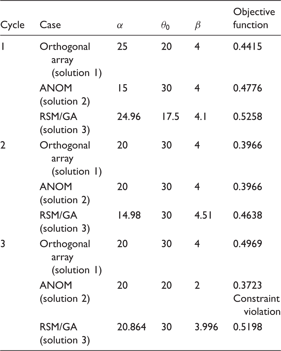
ANOM: analysis of mean; GA: genetic algorithm; RSM: response surface method.

Topology optimization in the structural discipline

Unsteady aeroelastic analysis is performed as the system analysis and the dynamic pressures of the wing surface are obtained from the system analysis. The pressures are imposed on the finite element model of the wing for topology optimization. The dynamic pressure is converted to the ESLs. ESLs are defined as the linear static load sets which generate the same response field in linear static analysis as that at a certain time of nonlinear dynamic analysis. The ESLs are made from the results of nonlinear dynamic analysis and used as external forces in linear static response optimization. Then the same response from nonlinear dynamic analysis can be considered throughout linear static response optimization. It is noted that the ESLs include the dynamic (inertia) effect of the structure.^34,52–56

Topology optimization is generally used to find the optimal layout of a structure within a specified region. ⁵⁷ The topology optimization method is classified into two methods. One is the homogenization method and the other is the density method. In the density method, design variables are the values for the artificial density function of the finite element. The density method based on the solid isotropic material with penalization is utilized for topology optimization. In this section, nonlinear dynamic response topology optimization using ESLSO is described. The design formulation and finite element model are explained.

Nonlinear dynamic topology optimization using ESLSO

ESLSO is adopted for nonlinear dynamic response topology optimization. The ESLs are static loads which generate the same displacement field in static analysis as the displacement field at each time step of nonlinear dynamic analysis. The ESLs are used in static optimization as external loads. Calculated ESLs at each time step are used as multiple loading conditions in topology optimization. The governing equation of nonlinear dynamic analysis is

$\mathbf{M}(\mathbf{b}){\stackrel{\mathrm{··}}{\mathbf{z}}}_{\text{N}}^t+\mathbf{C}(\mathbf{b}){\stackrel{·}{\mathbf{z}}}_{\text{N}}^t+{\mathbf{K}}_N({\mathbf{b}\mathbf{,}\mathbf{z}}_{\text{N}}^t){\mathbf{z}}_{\text{N}}^t=\mathbf{f}(t)\mathrm{\hspace{1em}\hspace{1em}\hspace{1em}}(t=t_0,t_1,\dots ,t_l)$

(11)

where $\mathbf{M}(\mathbf{b})$ is the mass matrix, $\mathbf{C}(\mathbf{b})$ is the damping matrix, ${\mathbf{K}}_{\text{N}}({\mathbf{b}\mathbf{,}\mathbf{z}}_{\text{N}}^t)$ is the stiffness matrix, ${\stackrel{\mathrm{··}}{\mathbf{z}}}_{\text{N}}^t$ is the acceleration vector, ${\stackrel{·}{\mathbf{z}}}_{\text{N}}^t$ is the velocity vector, ${\mathbf{z}}_{\text{N}}^t$ is the displacement vector, $\mathbf{f}(t)$ is the external load vector at the tth time step, and l is the total number of time steps in nonlinear dynamic analysis. The subscript “N” implies that the responses are obtained from the nonlinear dynamic analysis. The ESLs are calculated as

${\mathbf{f}}_{\mathrm{eq}}^s={\mathbf{K}}_{\text{L}}{\mathbf{z}}_{\text{N}}^s(s=1,2,\dots ,l)$

(12)

where ${\mathbf{f}}_{\mathrm{eq}}^s$ is the ESLs vector, ${\mathbf{K}}_{\text{L}}$ is the linear stiffness matrix, the notation s is matched with t in equation (11), and the subscript “L” means the value from linear analysis. The ESLs are calculated by multiplying the linear stiffness matrix and the displacement vector from nonlinear analysis. The number of ESLs is the same as that of the time steps.

ESLSO has been developed for size, shape, and topology optimizations.^{33,52–56,58} In this research, the method is applied to the structural design of the FWAV. The overall process of topology optimization using ESLSO is illustrated in Figure 17. The process is repeated until the convergence criterion is terminated. The repetition process is called a cycle. The steps of the nonlinear dynamic topology optimization using ESLSO are as follows:

Step 1. Set cycle number $k=0$ , the initial design variables ${\mathbf{b}}^{(k)}={\mathbf{b}}^{(0)}$ .

Step 2. Perform nonlinear dynamic analysis with ${\mathbf{b}}^{(k)}$ in equation (11).

Step 3. Calculate ESLs in the time domain by using equation (12).

Step 4. Perform linear static topology optimization with ESLs.

Step 5. Transform the values of the design variables into values of transformation variables using equation (13)

${\alpha }_i=\{0\mathrm{\hspace{1em}\hspace{1em}\hspace{1em}}\text{when}\mathrm{\hspace{1em}\hspace{1em}\hspace{1em}}{b}_i\le {\varepsilon }_{1}1\mathrm{\hspace{1em}\hspace{1em}\hspace{1em}}\text{when}\mathrm{\hspace{1em}\hspace{1em}\hspace{1em}}{b}_i>{\varepsilon }_1;\mathrm{\hspace{1em}\hspace{1em}\hspace{1em}}i=1,\dots ,n$

(13)

where ${\alpha }_i$ is the transformation variable for the ith corresponding design variables b_i. The total number of design variables and transformation variables is the same. The parameter ${\varepsilon }_1$ is a certain value between 0 and 1. If the value of the design variable is smaller than ${\varepsilon }_1$ , the corresponding transformation variable is regarded as 0. If not, the corresponding transformation variable has a value of 1. Thus, all design variables are replaced to 0 or 1 by using the transformation variable ${\varepsilon }_1$ .

• Step 6. Update the design. The elements, which have a transformation variable of value 1, remain in the finite element model. The elements, which have a transformation variable of value 0, are removed from the finite element model. The updated finite element model is used for nonlinear dynamic analysis in the next cycle.

• Step 7. When $k=0$ , go to Step 2 for the next cycle. Otherwise, check the convergence criterion.

Figure 17.

Process of topology optimization using ESLSO. ESLSO: equivalent static loads method for nonlinear static response structural optimization.

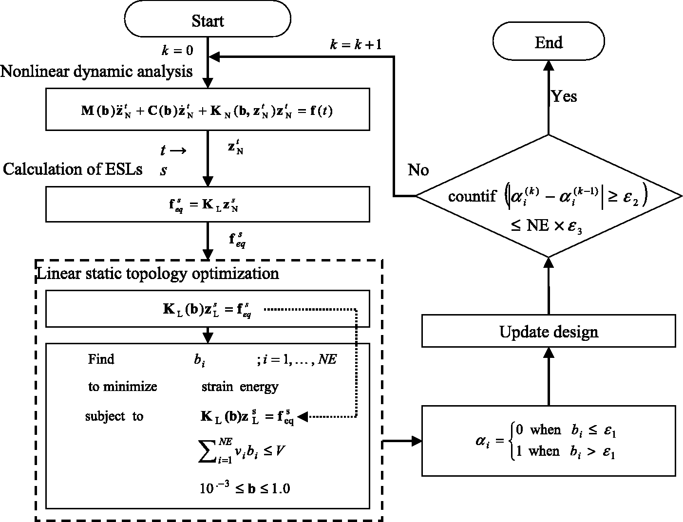
If the convergence criterion is satisfied, the optimization process terminates. If the convergence criterion is not satisfied, go to Step 2 of the next cycle. The convergence criterion is defined as

$\mathrm{countif}(|{\alpha }_i^{(k)}-{\alpha }_i^{(k-1)}|\ge {\varepsilon }_2)\le n\times {\varepsilon }_3$

(14)

where ${\varepsilon }_2$ is an arbitrary value between 0 and 1 and ${\varepsilon }_3$ is another user-defined small number. The number of design variables that change more than ${\varepsilon }_2$ is counted first. If the counted number is less than the certain value $n\times {\varepsilon }_3$ , then the process terminates. The topology result of the wing is applied to the structure model of the unsteady aeroelastic analysis (system analysis) of the next cycle.

ESLSO can perform nonlinear dynamic topology optimization using well-established nonlinear dynamic analysis and linear static response topology optimization.

Finite element model of the flapping wing

The surface pressures are obtained from the unsteady aeroelastic analysis (system analysis). The finite element model for topology optimization is generated from the structural model of unsteady aeroelastic analysis. The total number of the nodes and elements is the same as that of the structural model of the unsteady aeroelastic analysis. Figure 18 presents the finite element model of the wing. In the first cycle of the design process, the finite element model is the same for the system analysis and topology optimization. In the next cycle of the design process, the finite element model for the system analysis is changed because of the results of the topology optimization. The finite element model for topology optimization is still the same as the finite element model of Figure 18. In the topology optimization, the pressure condition of the wing surface is changed according to the results of the system analysis. In the initial FWAV model, the root of the leading edge is attached to the body frame as illustrated in Figure 1. Thus, the root of the wing is connected to one point by rigid elements. The boundary condition is imposed on the point and all the degrees of freedom in the six directions are fixed. The finite element model is composed of two shell element layers as illustrated in Figure 19. In Figure 19, the finite element model is divided into the design domain (carbon) and the nondesign domain (mylar). The density of an element in the design domain will have 0 or 1 in topology optimization while the density of the nondesign domain is always 1.

Figure 18.

Finite element model of the wing.

Figure 19.

Design domain and nondesign domain.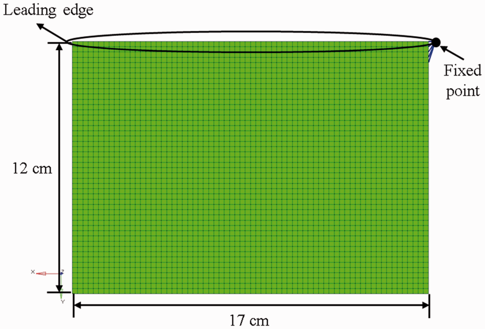

The design domain is the inner layer of the shell elements without the leading edge. One layer has 6760 shell elements. Common nodes are used for the outer and inner shell elements. The Young’s modulus of the design domain (carbon) is 170.3 GPa, the Poisson’s ratio is 0.3, and the material density is 2001.2 kg/m³. The Young’s modulus of the nondesign domain (mylar) is 3.28 GPa, the Poisson’s ratio is 0.4, and the material density is 1400.6 kg/m³. The thickness of the design domain is 0.5 mm and the thickness of the nondesign domain is 0.1 mm. The pressures are always imposed on the nondesign domain and the nondesign domain is supported by the design domain. Therefore, the topology of the reinforcement (carbon) is changed during the iteration of topology optimization. The dynamic surface pressures, which are obtained from the unsteady aeroelastic analysis, are applied to the nondesign domain of the finite element model at every time step of nonlinear dynamic analysis.

Design formulation for nonlinear dynamic topology optimization

In general, more flexible flapping wings are superior to stiffer wings. However, too much flexibility leads to a net drag, hence only a suitable amount of flexibility is desirable for thrust generation. The flapping wing structure should have some flexibility as well as certain rigidity, and a small amount of rigidity guarantees flexibility.^12,13,59 It means that the reduction of rigidity means an increase of the flexibility. In this research, the objective function is minimization of the strain energy and a constraint is defined for the specific value of the initial mass. It means that the objective function (strain energy) and the mass constraint can pursue rigidity and flexibility, respectively. Therefore, the maximum stiffness structure with a specific mass is obtained because it can support the aerodynamic force of the wing surface with the minimum mass. In other words, the wing structure has some flexibility because the stiffness of the structure is maximized while reducing the mass.

Nonlinear dynamic topology optimization using ESLs is formulated as follows

$\text{Find}{b}_i;\mathrm{\hspace{1em}\hspace{1em}\hspace{1em}}i=1,\dots ,\text{N\_DV}\text{to}\hspace{1em}\text{minimize}\text{strainenergy}\text{subject}\hspace{1em}\text{to}{\mathbf{K}}_{\text{L}}{(\mathbf{b})\mathbf{z}}_{\text{L}}^{\text{s}}-{\mathbf{f}}_{\text{eq}}^{\text{s}}=0\text{mass}\le {\text{mass}}_{\text{initial}}\times 30\%{10}^{-3}\le \mathbf{b}\le 1.0$

(15)

The design variable $b_i$ is the density of the $i\text{th}$ element in the design domain. The objective function is the summation of the strain energy at all the time steps. The constraint is that the mass of the structure should be less than 30% of the initial mass. $\text{N\_DV}$ is the number of design variables, which is 6644. The utilized software systems are LS-DYNA for nonlinear dynamic analysis, NASTRAN DMAP for calculating the ESLs, and OptiStruct for topology optimization.

Results of topology optimization

As mentioned earlier, nonlinear dynamic response topology optimization is performed to find the reinforcement of the wing structure. The dynamic pressure from the three-dimensional unsteady aeroelastic analysis is imposed on the flapping wing as the external loads. The summation of the strain energy is minimized in nonlinear dynamic topology optimization. If all the design variables are unchanged in the optimization, the optimization process is terminated. In nonlinear dynamic response topology optimization, mass fraction, ${\varepsilon }_1$ , ${\varepsilon }_2$ , and ${\varepsilon }_3$ are defined as 0.3, 0.5, 0.3, and 0.015, respectively. The results according to the cycle of the design process are illustrated in Figure 20. The remaining elements show the distribution of the reinforcement of the wing.

Figure 20.

Optimization results of the wing: (a) cycle 1, (b) cycle 2, and (c) cycle 3.

There are two cycles: one for the entire design process and one for ESLSO for topology optimization. The one for ESLSO is the inner cycle and the other is the outer cycle of the entire design process. If the entire design process converges in five cycles, the design process of Figure 4 is repeated five times. In the first cycle of the design process, nonlinear dynamic topology optimization converges in three cycles. That is, the design process of Figure 17 is repeated three times. Nonlinear dynamic topology optimization converges in three inner cycles in the second outer cycle of the design process. In the third outer cycle, nonlinear dynamic topology optimization converges in two inner cycles. The density value of the element is close to 1 when the color of the element is close to black. The reinforcement of the wing structure according to the progress of the outer cycle has more obvious outlines. After topology optimization, the shape of reinforcement is utilized in the structure model for three-dimensional unsteady aeroelastic analysis of the next outer cycle as illustrated in Figure 21. Consequently, the design process of Figure 4 converges in three cycles because all the design variables are unchanged in kinematic and structural optimizations.

Figure 21.

Application of the optimization results for the structured model.

As mentioned earlier, the initial model of Figure 1 is made by the results of some previous studies. The primary objective of the FWAV is the forward flight. A new FWAV is fabricated according to the optimization results. Components of the initial model, which consist of a motor, a receiver, a speed controller, and a battery, are also used for the optimized FWAV. The design variables for the initial model and optimized model are shown in Table 7. The weight is slightly increased because the reinforcement is increased in the optimized model. The maximum flapping frequency is decreased to 15 Hz due to the increase of the flapping amplitude. The two models are illustrated in Figure 22. This study shows the possibility of optimizing the flapping wing system. The kinematic and structural disciplines are simultaneously optimized to consider the flexibility of the wing. In the future, it will be necessary to establish the experimental system and the test method for the performance comparison.

Table 7.

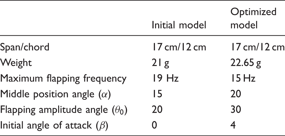
Comparison of the initial model and the optimized model.

	Initial model	Optimized model
Span/chord	17 cm/12 cm	17 cm/12 cm
Weight	21 g	22.65 g
Maximum flapping frequency	19 Hz	15 Hz
Middle position angle (α)	15	20
Flapping amplitude angle ( ${\theta }_0$ )	20	30
Initial angle of attack (β)	0	4

Figure 22.

Flapping wing air vehicle: (a) initial model and (b) optimized model.

Conclusions

A design process is defined for optimization of the flapping wing system by using MDO. The design process consists of the system analysis, the aerodynamic discipline, and the structural discipline. From the system analysis, the deformed shapes of the wing are transferred to the fluid discipline and the dynamic pressures are transmitted to the structural discipline. In the fluid discipline, kinematic optimization is conducted to enhance the performances such as the thrust and propulsive efficiency. The OA, ANOM, RSM, and GA are employed for optimization and two-dimensional aerodynamic analysis for a two-dimensional airfoil is utilized for the optimization process. In the structural discipline, ESLSO is utilized for nonlinear dynamic response topology optimization of the wing structure. The strain energy is minimized to find the stiffest structure with a specific mass. The external loads are calculated from three-dimensional aeroelastic analysis. The design process is applied to a real FWAV model. The results of kinematic optimization and topology optimization are obtained. The optimized FWAV model is fabricated based on the optimization results.

Consequently, a design process that utilizes MDO is proposed. The design process is applied to a design problem of FWAV. The number of costly unsteady aeroelastic analysis is reduced. Thus, the design process can be applied to various problems of flapping wing. The defined design process may be of benefit when designing the flapping wing system of an FWAV. In the future, the experimental system and the experiment method will be studied for comparison of the performance. Besides, this research will be expanded to the design of various FWAVs to accommodate the hovering flight, the maneuverability flight, the efficient flight, etc.