Sage Journals: Discover world-class research

Abstract

Future integration of small unmanned aircraft within an urban airspace requires an a posteriori understanding of the building-induced aerodynamics which could negatively impact on vehicle performance. Moving away from generalised building formations, we model the centre of the city of Glasgow using Star-CCM+, a commercial CFD package. After establishing a critical turbulent kinetic energy for our vehicle, we analyse the CFD results to determine how best to operate a small unmanned aircraft within this environment. As discovered in a previous study, the spatial distribution of turbulence increases with altitude. It was recommended then that UAVs operate at the minimal allowable altitude within a congested area. As the flow characteristics in an environment are similar, regardless of inlet velocity, we can determine areas within a city which will have consistently low or high values of turbulent kinetic energy. As the distribution of turbulence is dependent on prevailing wind directions, some directions are more favourable than others, even if the wind speed is unchanging. Moving forward we should aim to gather more information about integrated aircraft and how they respond to turbulence in a congested area.

Keywords

CFD Urban Aerodynamics Nonlinear Control Quadrotor Dynamics

Introduction

Considering the significant increase in the number of commercially available multi-rotor vehicles, as well as the interest expressed by businesses to implement these devices for a wide range of purposes, it would seem then that UAV integration within an urban environment is inevitable. This paper aims to highlight some of the issues facing multi-rotor platforms on the path to their eventual certification for low-level, urban operation. Currently, regulations concerning the operation of commercially and privately owned vehicles are broad. The Civil Aviation Authority’s ANO 2009 defines any unmanned aircraft with an operating mass of less than 20 kg as a ‘Small Unmanned Aircraft’.¹ The implication of this classification is that such vehicles are exempt from the majority of regulations which would apply to manned aircraft. For the small unmanned aircraft, this means that both airworthiness approval and registration are not required. However, this classification imposes limitations on these vehicles to prevent them from: flying in congested areas; flying close to people or property and flying beyond visual line of sight. ANO 2009 further states that ‘a person shall not recklessly or negligently cause or permit an aircraft to endanger any person or property'. Specifically for flight in an urban environment, CAP 722² grants permission for aircraft of less than 7 kg to be flown, but no closer than 50 m to the nearest person or structure. Vehicles with a mass greater than 7 kg but less than 20 kg are not normally allowed to fly in congested areas at all, unless special permission is granted by the CAA.

Quantification of these operational constraints does not take into account either the prodigious advance in affordable platform autopilot systems or the maturity of advanced non-linear control laws refined for the small UAV application. The problem with simply maintaining the existing CAA operational requirements is that many of the commercial and homeland security tasks that could conceivably be offloaded to small UAVs require much closer operation to both persons and property – tasks such as close building inspection, small package delivery & precise tracking/surveillance of persons-of-interest. Given the current operational restrictions and the impact those have on potential commercial exploitation of UAV technology, it is imperative that research is carried out to specifically quantify the robustness of these vehicles in all operational conditions.

One of the main obstacles facing the establishment of a comprehensive regulatory framework is quantifying the ability of autonomous vehicles to perform adequately in a turbulent urban environment. The problem which arises is the understanding of fluid flow within a space of non-uniformly distributed structures of varying geometries. If we consider a potentially worldwide distribution of multi-rotor vehicles operating in urban areas, the scale of the problem becomes evident. However, efforts into researching the impact of building induced turbulence on such vehicles remains in its infancy

In an attempt to demonstrate the considerations that we must make when integrating small, unmanned aircraft within an urban environment, we have modelled a section of the centre of the city of Glasgow, within the commercial CFD package Star-CCM+. Whilst some work has approached the subject of UAV flight in a turbulent urban environment,³ most studies which model urban aerodynamics tend to focus on areas such as pedestrian comfort and pollutant dispersion.^4–6

Previous research by Murray and Anderson⁷ focused on the determination of 3D paths through a generic urban environment. By utilising CFD results of flow in this environment, we established that the variation in turbulent kinetic energy (TKE) was such that there were regions that would be severely detrimental to quadrotor operations. These areas were defined as possessing critical TKE values. By mapping an urban environment in terms of its critical TKE, safe paths were generated which avoided these areas and minimised the impact of turbulence on the vehicle dynamic response.

The intent of this study is to provide a qualitative analysis of the spatial variation of critical TKE in a realistic environment. If the future integration of small or micro-UAVs within an urban landscape is to be realised, our understanding of the complex aerodynamic interactions that will impact these vehicles must be increased.

Environmental modelling

Representation of urban environment

The buildings present in an urban environment can be generalised and classified as three main types, characterised by the flow around them, based on the building height, H and windward width, a_w. These classifications are outlined in Table 1 and an illustration of their application is shown in Figure 1.

Table 1.

Building classifications.

	Height/width relationship
Tall building	H > 1.25a_w
Tall building of transitional type	0.33a_w ≤ H ≤ 1.25a_w
Long face	a_w > 3H

Figure 1.

Building geometry and separation.

Just as there are three flow types for single buildings of varying height and windward width, there are also three separate flow classifications for twin building configurations. These classifications are defined by the aspect ratio of the buildings, W/H, where H is the building height and W is the street width. Table 2 highlights the differences in flow characteristics based on the aspect ratio of twin buildings.

Table 2.

Flow definition as a function of aspect ratio.

	Aspect ratio
Isolated Roughness	W/H > 1.25
Wake Interference	1.54 ≤ W/H ≤ 3.30
Skimming flow	W/H < 1.54

The details of flow characteristics surrounding the single and twin building configuration are well established in the literature.^8–11 Whilst these generalisations are useful in understanding flow behavior in an urban environment, as the layout of a cityscape becomes increasingly complicated, we have to rely on these representations less and less as we move towards a fuller understanding of urban flow characteristics for the purpose of airspace integration of small unmanned aircraft.

Discretisation of the fluid domain and validation of the CFD results, as well as a discussion of the difficulties encountered when modelling large scale flow fields, are outlined in a previous paper by Murray et al.¹² The size of the domain was determined using guidelines published by Franke et al.,¹³ and a logarithmic inlet velocity profile was created

u = \frac{u_{*}}{κ} [\ln (\frac{z - d}{z_{0}})]

(1)

To create our logarithmic inlet profiles, we consider two wind speeds, measured at a height of 10 m: $U_{10}$ = 5 m/s and $U_{10}$ = 10 m/s. The smaller value represents an average wind speed for Glasgow, measured at a local weather station. The larger value is a more extreme representation of wind speed magnitudes we may expect. The urban wind speeds themselves are a function of the environmental layout. Whilst we can readily obtain atmospheric data for the CFD boundary conditions, it is harder to define typical wind speeds without the utilisation of numerical simulation.

Just as we require a velocity profile for the inlet boundary condition, we have found the most success in using an inlet profile for the turbulence dissipation rate also,¹⁴ as well as a constant value for the TKE inlet condition

ɛ = \frac{u_{*}^{3}}{κ (z + z_{0})}

(2)

k = 1.5 u_{*}^{2}

(3)

The majority of research which characterises urban flow, in relation to pollutant dispersion and pedestrian comfort, can be used to assess which models are most appropriate for the operating environment of a quadrotor. Although the applications are varied, the literature provides insight into which approaches most accurately represent the turbulent urban environment.

Comprehensive research has been conducted into the validity of models such as the standard $k - ɛ$ , RNG $k - ɛ$ and the Reynolds-Stress model. Comparison of wind tunnel tests with numerical solutions demonstrates that the Reynolds-averaged models predict key flow characteristics such as rooftop recirculation.¹⁵ However, as the solution is steady state, it cannot account for transient effects such as the intermittency of the flow circulation and its redevelopment.

Although some early studies cited the Reynolds-stress model as being the most accurate in its prediction of pollutant concentration, it has often performed poorly in comparative studies of turbulence models.¹⁶ Thus, comparisons of modelling approaches tend to focus on the standard $k - ɛ$ model and its variants.

With pure consideration of linear eddy viscosity models applied to urban pollutant dispersion, the RNG $k - ɛ$ approach was found to be the most accurate when predicting concentration levels, which implies an accurate prediction of the velocity flowfield, as a result.¹⁷ However, if one were to utilise commercial code which did not make use of the RNG $k - ɛ$ model, such as Star-CCM+, the realisable and Kato-Launder modification approaches would work equally as well.¹⁷ For our simulation, we have adopted a segregated, steady solver and a realisable $k - ɛ$ turbulence model to capture the flow characteristics.

The time-averaged Navier-Stokes equations provide a statistical description of flow in an urban environment. With regard to flowfield generation, comparisons between experimental and numerical results yield weaknesses in the predictive capabilities of the RANS methods. This is due to the inability of the steady RANS computation to account for large scale fluctuations such as vortex shedding.^18,19 One solution would be to adopt unsteady approaches such as unsteady-RANS or large eddy simulation (LES). However, with regard to the study of a turbulent urban airspace, such approaches are far more computationally intensive. Given that we may one day wish to generate banks of numerical turbulence data for defining the operating environment of a small-UAV, utilisation of RANS models will facilitate the accomplishment of this feat in a relatively short timeframe, with acceptable accuracy.

Meshing

The domain is discretised into 843,703 hexahedral cells. Star-CCM+ allows the user to specify a base mesh size for the entire domain and then create block parts, where the mesh can be refined. In each of these parts, the mesh size is defined as a percentage of the base. Figure 2 shows the block parts that are used to refine the mesh around areas where a sufficiently high mesh density is required to capture all flow features. It also shows a plane section of the mesh which illustrates the change in the size of the hexahedral cells as the base size of the far field domain transitions to the finer mesh of the regions surrounding the buildings. Table 3 contains the size of the mesh in the far field domain and each of the block regions.

Figure 2.

Discretisation of fluid domain and refinement of mesh.

Table 3.

Hexahedral cell size in each region.

	Cell size (% of base)	Absolute cell size (m)
Domain (base size)	100	20
Block 1	60	12
Block 2	20	4

Vehicle dynamics

Rigid body dynamics

The dynamics of the quadrotor are covered extensively in literature and will be briefly described here. For a greater description of the system, see Ireland and Anderson.²⁰ The linear and angular velocities of the aircraft are described in a body-fixed frame of reference $B$ by the non-linear relationships

m \overset{\cdot}{v} = R_{W}^{B} [00 mg] - [00 \sum T] - ω \times mv

(4)

I \overset{\cdot}{ω} = [L (T_{3} - T_{4}) L (T_{2} - T_{1}) - Q_{1} - Q_{2} + Q_{3} + Q_{4}] - ω \times I ω

(5)

These are related to the position r and attitude η of the vehicle in an inertially-fixed world frame $W$ by the kinematic relationships

\overset{\cdot}{r} = R_{B}^{W} v

(6)

\overset{\cdot}{η} = R_{η} ω

(7) where the transformation matrices

R_{B}^{W}

and

R_{η}

are given by

R_{B}^{W} = [\cos θ \cos ψ \sin φ \sin θ \cos ψ - \cos φ \sin ψ \cos φ \sin θ \cos ψ + \sin φ \sin ψ \cos θ \sin ψ \sin φ \sin θ \sin ψ + \cos φ \cos ψ \cos φ \sin θ \sin ψ - \sin φ \cos ψ - \sin θ \sin φ \cos θ \cos φ \cos θ]

(8)

R_{W}^{B} = (R_{B}^{W})^{T}

(9)

R_{η} = [1 \sin φ \tan θ \cos φ \tan θ 0 \cos φ - \sin φ 0 \sin φ \sec θ \cos φ \sec θ]

(10)

The inertially-fixed frame of reference $W$ is represented by a mutually orthogonal set of right-handed axes. By adopting the north east down (NED) convention, the positive x-axis points north, the positive y-axis points east and the positive z-axis points down, aligned with the direction of the gravitational acceleration. The body-fixed frame of reference $B$ is also represented by an orthogonal set of right-handed axes, whose origin is coincident with the vehicle centre of gravity. Figure 3 illustrates the quadrotor vehicle and its frames of reference.

Figure 3.

Principal thrusts and torques acting on a quadrotor platform in a body-fixed reference frame, relative to an inertially-fixed world frame.²¹

The derivation of the thrust and torque variables, T and Q, will be expanded upon in the following section. It is through these terms that axial and angular perturbations are transmitted, resulting from the changes in rotor inflow caused by the variation in the component vector magnitude of the gust field.

Rotor inflow model

To accurately include the effects of turbulence on a quadrotor platform, a rotor inflow model was created to simulate the variation in thrust produced by changes in the inflow velocity, resulting from the translation of the quadrotor within a turbulent urban environment. The equations in this section are modified from the works of Leishman²² and Fay.²³ Whilst these approaches can be utilised independently of one another, we have combined both formulations. As well as accounting for the hub-fixed gust components, the value of the thrust coefficient, whose expression was derived by Fay,²³ is updated during the Newton-Raphson procedure outlined by Leishman.²²

Considering $u, v$ and w are the body-fixed translational velocities, we can define the edgewise velocity of the rotor to be

V = \sqrt{(u - G_{x})^{2} + (v - G_{y})^{2}}

(11)

The inclusion of the hub-fixed gust components, G_x and G_y, within the definition of the edgewise rotor velocity ensures that even if the quadrotor is hovering, climbing or descending, the longitudinal and lateral components of the gust field will still have an effect on the calculation of thrust.

We can now introduce a quantity known as the rotor advance ratio which is simply expressed as the edgewise velocity, V, normalised by the rotor tip speed, $Ω R$

μ = \frac{V}{Ω R}

(12)

The thrust produced by a rotor is determined by the rate of change of momentum across the rotor disk

T = \overset{\cdot}{m} Δ v

(13) where

\overset{\cdot}{m}

is the mass flow rate and

Δ v

is the change in velocity between the region far above the rotor, assumed to be at rest, and the far downstream wake. Application of the conservation of momentum in a direction normal to the disk, as well as the conservation of energy, results in a relationship between the rotor thrust and the induced velocity at the disk. The total inflow velocity comprises of an induced component, hub-fixed vertical motion component and a hub-fixed gust component. It is non-dimensionalised by the rotor tip speed and expressed as the total inflow ratio, λ

λ = \frac{v_{i} - w - G_{z}}{Ω R}

(14)

λ_{i} = \frac{v_{i}}{Ω R} = \frac{C_{T}}{2 \sqrt{μ^{2} + λ^{2}}}

(15) where

λ_{i}

is the induced inflow ratio, the component of the inflow resulting from the rotation of the propeller blades, neglecting external velocity sources such as vehicle motion and gust contributions.

The propeller blades are assumed to be rigid and the disk is oriented normal to the rotor shaft. As the positive, body-fixed z-axis of the quadrotor acts in the same direction as the induced flow, the body-fixed vertical velocity component will be negative when the vehicle climbs. Thus, the formulation of equation (14) reflects the fact that a negative vertical body velocity, w, will contribute positively to the total inflow. Combining equations (14) and (15)

λ = \frac{C_{T}}{2 \sqrt{μ^{2} + λ^{2}}} - \frac{w - G_{z}}{Ω R}

(16)

A value for the inflow ratio can now be obtained by solving equation (16) using a Newton-Raphson method, as described by Leishman. An iterative solution is necessary as the thrust varies as a function of inflow and vice versa. The only difference between the numerical approach applied in this paper and that of Leishman is that the convergence criterion is based on the thrust coefficient instead of the inflow ratio

ε = \frac{C_{T_{n + 1}} - C_{T_{n}}}{C_{T_{n + 1}}}

(17)

\frac{C_{T}}{σ a} = (\frac{1}{6} + \frac{1}{4} μ^{2}) θ_{0} - (1 + μ^{2}) \frac{θ_{tw}}{8} - \frac{1}{4} λ

(18)

T = ρ {AC}_{T} (Ω R)^{2}

(19)

Once the solution has converged, thrust is calculated using equation (19). Obtaining values for the torque coefficient is now straightforward, after solving the inflow equation

\frac{C_{Q}}{σ a} = \frac{1}{8 a} (1 + μ^{2}) \bar{C_{d}} + λ (\frac{1}{6} θ_{0} - \frac{1}{8} θ_{tw} - \frac{1}{4} λ)

(20)

Q = ρ {AC}_{Q} (Ω R)^{2} R

(21)

Modelling of the propeller aerodynamics

The propeller model in this study is based on the APC Slow Flyer 10″ × 4.7″ and experimental performance data are obtained from the work of Brandt and Selig.²⁴ Based on their measurements of the blade geometry, we can obtain values for the solidity ratio, σ and the linearised blade twist parameters

θ = θ_{0} - θ_{tw} (\frac{r}{R})

(22) where

θ_{0}

is the collective pitch and

θ_{tw}

is the blade twist rate.²² Whilst

θ_{0}

and

θ_{tw}

can be calculated from the geometry of the propeller, the lift curve slope, a, can usually be defined as equal to

2 π

, according to thin airfoil theory. However, examining Figure 4, constant lift–curve slope values will result in model inaccuracies over a range of advance ratios. This could be due to the assumptions made when deriving the expressions for the thrust and torque coefficients, such as uniform inflow across the disk and rigid propeller blades. Additionally, increased accuracy in blade element modelling has been observed by: taking 3D equilibrium into account; applying 3D correction factors which account for losses arising from tip and root vortices and by implementing a post stall model.^25,26 Rather than including a greater physical description of the aerodynamics into our model, we have opted to further increase the fidelity by augmenting the lift–curve slope term, such that the performance of our numerical model emulates experimental observation.

Figure 4.

Comparison of experimental measurements of thrust coefficient varying with vertical advance ratio against numerical inflow model with constant lift–curve slope term.

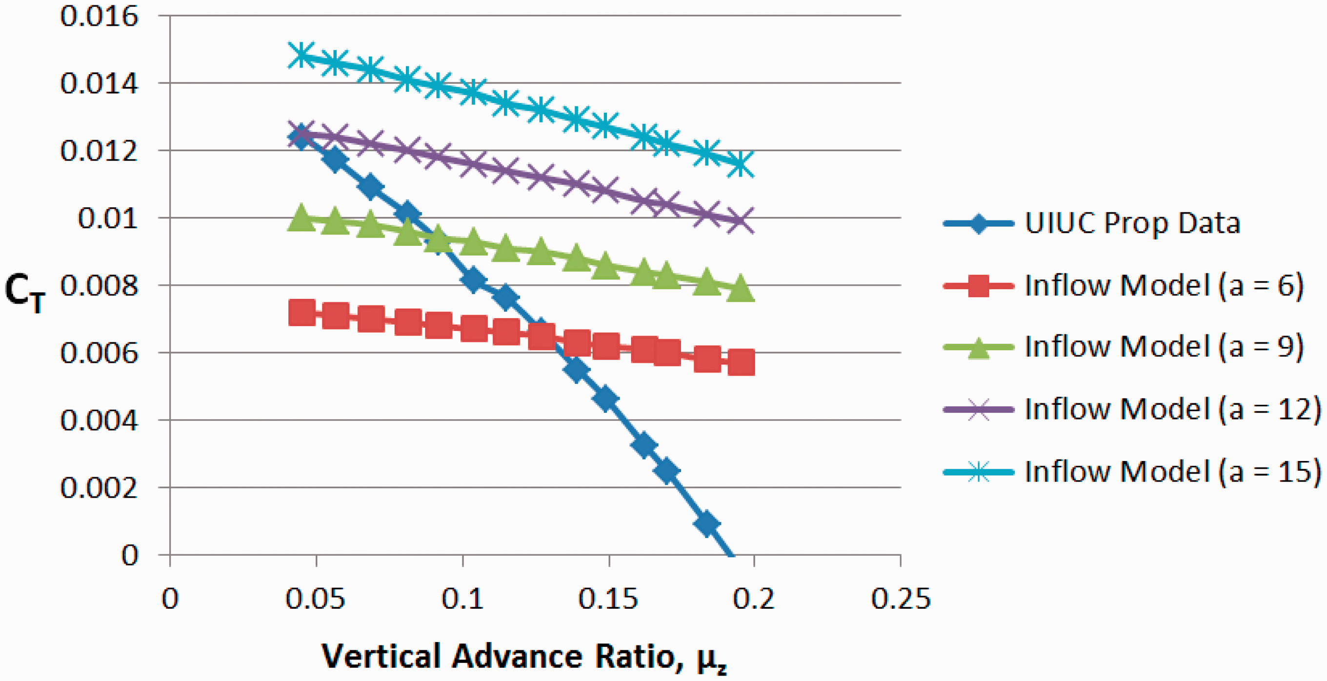
Whilst we recognise that such empirically derived expressions have no real physical meaning, they serve to encapsulate all the un-modelled effects and provide accurate performance results for variations in local flow conditions. This is the most important consideration when assessing the dynamic response of a small UAV in a turbulent environment. Also note that modelling inaccuracies are observed with: variations in RPM; increasing horizontal advance ratio and changes in descent velocity. Thus, we will now outline the procedure for the derivation of the augmented lift–curve slope terms.

Beginning with the variations in RPM, the value for a is continually modified until the thrust coefficient matches that of the experimental value, for the same propeller angular rate. Repeating this procedure, over a range of RPM values, yields an approximately linear relationship between a and RPM that can be expressed as follows

a_{rpm} = 0.001 Ω_{rpm} + 9.785

(23)

For the relationship between the vertical advance ratios and the lift curve slope, just as before, we can modify the value of a until our desired performance parameters match. As previously discussed, w does not represent the descent speed but the body-fixed vertical velocity of the quadrotor. As such, its value can be either positive or negative. When it is positive, this corresponds to vehicle descent and a negative value indicates that the vehicle is climbing. The combination of the body-fixed velocity and the local vertical gust magnitude will determine whether or not the resultant velocity will act in the same direction as the induced flow or against it. Thus, the vertical advance ratio can be expressed in two directions, $μ_{z}$ for velocities which contribute to the total inflow and $μ_{- z}$ for velocities which reduce the total inflow. The consideration of variations in $μ_{- z}$ is important as large values could result in the onset of the vortex ring state. We will address this concern after we have derived the appropriate empirical expressions for the lift slope. Maintaining constant RPM and increasing $μ_{z}$ , where

μ_{z} = \frac{w - G_{z}}{Ω R}

(24)

Thus, the relationship between a and the vertical advance ratio can be expressed as

a_{μ_{z}} = - 59.176 μ_{z}^{4} + 77.253 μ_{z}^{3} - 48.929 μ_{z}^{2} - 8.5752 μ_{z} + 0.007

(25)

For variations in the negative vertical advance ratio

a_{μ_{- z}} = 63544 a_{μ_{- z}}^{6} - 112989 a_{μ_{- z}}^{5} + 74471 a_{μ_{- z}}^{4} - 21756 a_{μ_{- z}}^{3} \dots + 2687.3 a_{μ_{- z}}^{2} - 97.817 a_{μ_{- z}} - 0.0093

(26)

Finally, determining the relationship between the lift curve slope and horizontal advance ratio from equation (12) by the same means

a_{μ} = - 136192 μ^{5} + 105144 μ^{4} - 29592 μ^{3} + 3577.3 μ^{2} - 130.93 μ + 0.0016

(27)

Combining equations (23), (25), (26) and (27)

a = a_{rpm} + a_{μ} + a_{μ_{z}} + a_{μ_{- z}}

(28)

Thus, by consolidating the four separate lift curve slope terms, after deriving them from empirical results, we can turn a simple uniform inflow model into an accurate representation of any propeller we wish. Note that the above polynomial lift curve expressions apply only to the APC Slow Flyer 10″ × 4.7″. Figure 5 demonstrates the accuracy with which the propeller performance is emulated when the augmented lift–curve slope terms are included. The only experimental data not collected by Brandt and Selig²⁴ is the variation in thrust coefficient with advance ratio. Those experiments were conducted within the Aerospace Sciences Research Division at the University of Glasgow.

Figure 5.

Variation in thrust coefficient with variations in: RPM; advance ratio; vertical advance ratio and negative vertical advance ratio.

Regarding the onset of the vortex ring state, the bottom right hand portion of Figure 4 illustrates the variation in performance, whilst operating in this condition. However, the vortex ring state is characterised by unsteadiness of the induced velocity, which is not evident as the experimental results were time averaged. Whilst the empirical expressions for inflow do exist, they also lack a description of the transient phenomena. Therefore, our expression for the variations in thrust coefficient due to increasing negative vertical advance ratio, from vortex ring state to the windmill brake state, is of suitable accuracy.

Furthermore, consider operational conditions where the application of momentum theory is still semi-valid²²

- 0.25 \leq \frac{w}{v_{h}} < 0

(29) where v_h is the induced velocity in hover. The mass of the vehicle is

m = 1.54

kg. Therefore, the thrust required by a single rotor in hover is

T = 3.78

N. The induced velocity in hover is then calculated using the following expression

v_{h} = \sqrt{\frac{T}{2 ρ A}}

(30) where ρ is the density of air and A is the area of the rotor disk. Thus, the induced velocity in hover is

v_{h} = 5.52

m/s. This implies that the maximum descent velocity achievable, before momentum theory assumptions break down completely is

w = 1.38

m/s, which is a reasonably rapid descent when considering quadrotor flight. It may then be that momentum theory assumptions hold and the onset of the vortex ring state can be avoided, for a wide range of operating conditions. However, if rapid descent is required, or the vehicle interacts with a strong vertical gust, the empirical relationship which was determined earlier should still provide acceptable performance predictions.

Statistical modelling of the temporal variation of velocity components

The CFD results are Reynolds-averaged, meaning that they do not possess any transient properties. However, turbulence is characterised by its unsteady behaviour. To resolve this issue, we can approximate the unsteadiness by employing a Dryden continuous gust model, a statistical approach to obtain the velocity fluctuations associated with turbulent conditions. This is particularly useful when using it in combination with a rotor inflow model as it is less computationally intensive, loading a single array of numerical CFD data as opposed to multiple arrays, one for each time step.

Extracting the TKE data from the Star-CCM+ simulations, we can define the relationship between k and the root-mean-square of the turbulent velocity fluctuations, $u'$ , as

u' \equiv \sqrt{\frac{1}{3} (u'_{x}^{2} + u'_{y}^{2} + u'_{z}^{2})} = \sqrt{\frac{2}{3} k}

(31)

Thus, a Dryden PSD can be created for longitudinal, lateral and vertical directions using the following equations²⁷

Φ_{v, w} (ω) = σ^{2} \frac{L_{g}}{π V_{QR}} \frac{1 + 3 (\frac{L_{g} ω}{V_{QR}})^{2}}{(1 + (\frac{L_{g} ω}{V_{QR}})^{2})^{2}}

(32)

Φ_{u} (ω) = σ^{2} \frac{2 L_{g}}{π V_{QR}} \frac{1}{(1 + (\frac{L_{g} ω}{V_{QR}})^{2})^{2}}

(33) where

σ = u'

and subscripts u, v and w represent the longitudinal, lateral and vertical directions, respectively. Once the PSD has been obtained, a time history can be created

G (t) = \sum_{m = 1}^{\infty} \sqrt{Φ (ω_{m}) Δ ω} \cos (ω_{m} t + ψ_{m})

(34) where

G (t)

is the magnitude of the gust velocity fluctuation about the mean velocity value.

Using this method, a transient term can be directly incorporated within our inflow model. Thus, at every time step, the gust magnitude will change, invoking an unsteady dynamic response. Additionally, as the magnitude of the PSD is determined by the TKE, fluctuations are greatest in areas where k is highest. The random nature of equation (34) also implies that even in hover, the quadrotor will be affected by the turbulence in such a way that we should observe axial and angular changes in its position.

Performance of quadrotor under the influence of atmospheric turbulence

Problematic areas in our environment are considered to contain values of critical TKE. At this point, we should define what we mean by a critical TKE value. Consider a quadrotor, or indeed any micro-UAV, operating in turbulent conditions where, as discussed earlier, there exist large temporal variations in velocity that are proportional to the square root of the magnitude of the local TKE value. In this environment, the control system of the autonomous vehicle attempts to mitigate the negative effects arising from the aerodynamic interaction between our micro-UAV and the turbulent conditions. As the TKE increases, the magnitude of the variation in velocity increases also. As a result, we observe larger vehicle displacements and increased changes in vehicle attitude. Once these deviations are sufficiently large, such that they exceed any imposed operational requirements, or if the control inputs are saturated and the vehicle becomes unstable, we can define the associated TKE as being the vehicle’s critical value. When operating in a turbulent urban environment, the objective becomes the maximisation of this critical value. If the increased turbulence does not cause our quadrotor to become unstable, then we must come up with a definition of what we consider to be its critical TKE value, based on operational metrics which we can use to assess the performance of a micro-UAV in an environment dominated by large, temporal variations in its flowfield. One such metric that we have considered is the boundedness of the vehicle. A term more commonly encountered in mathematics, we have used it here to describe spatial limits imposed on the vehicle. For the hovering UAV, this could be a requirement which states that movement is restricted to 1 m in each direction, for example. This creates a deviation sphere with a radius of 1 m, where the desired quadrotor position is at the centre. If the turbulence is such that the vehicle cannot stay within these virtual confines, then it has performed poorly based on the concept of boundedness. Although it has not become unstable, the point at which it fails to stay within these limits can be used to define the critical TKE also, as the performance of the autonomous quadrotor has not met operational requirements. Of course, such performance metrics can be defined to possess any value deemed necessary by the user. For this investigation, we will use the bounded criteria of 1 m in any direction as a judge of the controlled quadrotor performance.

Figure 6 demonstrates the dynamic response of a quadrotor hovering in turbulent conditions, influenced by two separate TKE values. Table 4 contains the maximum displacement from the desired hovering position in the X and Y directions. Displacement in the Z direction is not recorded as we can see from Figure 6 that the quadrotor is quite stable when maintaining a prescribed altitude.

Figure 6.

Top quadrotor response (TKE = 6 J/kg) bottom: quadrotor response (TKE = 9 J/kg).

Table 4.

Maximum values of displacement in X and Y directions.

TKE (J/kg)	+X (m)	−X (m)	+Y (m)	−Y (m)
6	1.1978	−0.8616	0.5724	−0.8333
9	1.6059	−1.6294	1.4246	−2.1218

Thus, we can ascertain from this data that our vehicle’s critical TKE value lies somewhere between 6 J/kg and 9 J/kg. Although the quadrotor exceeded its spatial boundary in the positive X direction only, for the lowest kinetic energy value simulated, this would be enough to declare that the quadrotor has not adhered to operational requirements. In fact, we should say that as a result of this, the critical TKE value is defined as the first instance when the vehicle has not performed according to the boundedness metric. Therefore, for the purposes of this investigation, we have assigned our vehicle with a critical TKE value of 6 J/kg, a value which is applicable only to the quadrotor that has been modelled for this investigation. It is a function of an individual vehicle’s properties, such as mass and moments of inertia, as well as the control strategy that has been adopted. Therefore, a vehicle operating in a turbulent urban environment could feasibly have a different critical TKE value from the other aircraft. If the mass of the aircraft were to be increased, larger forces would be required to elicit the kind of dynamic response that would cause it to become unstable. Thus, you could determine immediately that such a vehicle would have a larger operating TKE range than its smaller counterparts.

Quadrotor control

Control of the quadrotor is achieved using feedback linearisation, which allows the linearised closed-loop system to be tuned to provide a desired response. The control system uses a nested feedback loop configuration, where the attitude controller is informed by commands from the position controller.

Position control

Height control is achieved using the non-linear control law

u_{col} = \frac{m (g - {\overset{··}{Z}}_{d})}{K_{T} \cos φ \cos θ}

(35) where

{\overset{··}{z}}_{d}

is the desired acceleration in z and is determined by the state feedback law

{\overset{··}{Z}}_{d} = K_{z 1} (z_{d} - z) - K_{z 2} \overset{\cdot}{z}

(36)

The gain K_T is based on a linear model of the rotor system and relates the thrust of each rotor to its input u by $T_{i} = K_{T} u_{i}$ .

The roll and pitch commands for the attitude controller, $φ_{d}$ and $θ_{d}$ respectively, are obtained from the linearising feedbacks

φ_{d} = - a \sin \frac{m ({\overset{··}{x}}_{d} \sin ψ - {\overset{··}{y}}_{d} \cos ψ)}{K_{T} u_{col}}

(37)

θ_{d} = - a \sin \frac{m ({\overset{··}{x}}_{d} \cos ψ + {\overset{··}{y}}_{d} \sin ψ)}{K_{T} u_{col} \cos φ}

(38) where the desired accelerations in x and y are determined by the state feedback laws

[{\overset{··}{x}}_{d} {\overset{··}{y}}_{d}] = K_{xy 1} ([x_{d} y_{d}] - [x y]) - K_{xy 2} [\overset{\cdot}{x} \overset{\cdot}{y}]

(39)

The gains $K_{z 1}$ , $K_{z 2}$ , $K_{xy 1}$ and $K_{xy 2}$ are obtained from comparison of the linearised closed-loop systems with a desired second-order system.

Attitude control

Attitude control is achieved similarly, using the linearising feedbacks

u_{lat} = \frac{I_{x} {\overset{\cdot}{p}}_{d} + (I_{z} - I_{y}) qr}{K_{T} L}

(40)

u_{long} = \frac{I_{y} {\overset{\cdot}{q}}_{d} + (I_{x} - I_{z}) pr}{K_{T} L}

(41)

u_{yaw} = \frac{I_{z} {\overset{\cdot}{r}}_{d} + (I_{y} - I_{x}) pq}{K_{Q}}

(42) With the state feedback laws

[{\overset{\cdot}{p}}_{d} {\overset{\cdot}{q}}_{d} {\overset{\cdot}{r}}_{d}] = K_{η 1} ([φ_{d} θ_{d} ψ_{d}] - [φ θ ψ]) - K_{η 2} [p q r]

(43)

The gains $K_{η 1}$ and $K_{η 2}$ are obtained from comparison of the linearised closed-loop systems with a desired second-order system.

Generic environment vs. existing cityscape

In a previous investigation,¹² it was demonstrated that the turbulence generated by various building configurations can have a detrimental impact on the operation of a small UAV. Therefore, we cannot plan routes through an urban environment without first taking into consideration the variation in turbulence intensity that degrades vehicle performance. Implementing the A* algorithm, routes through 2D and 3D environments that avoided areas of increased turbulence were obtained. This knowledge of the variation of TKE throughout an urban environment provided us with a necessary first step towards the eventual integration of autonomous rotorcraft within a small to large city. However, the most complex building configuration analysed was a ‘plus’ configuration of four tall buildings of equal height, as shown in Figure 7.

Figure 7.

Spatial variation of TKE for the ‘Plus’ configuration.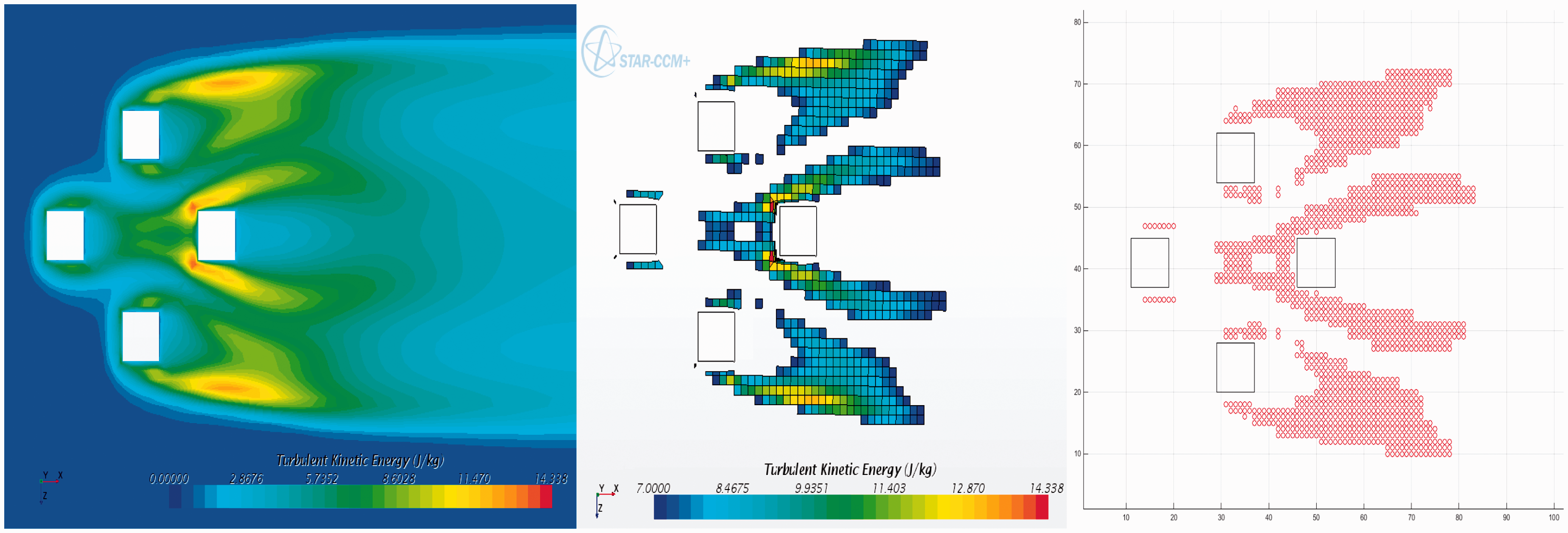

We can see that the symmetrical nature of this simplified urban environment generates symmetrical flow profiles with clearly defined corridors of low TKE that are considered navigable when utilising a 2D A* algorithm or some other optimal guidance scheme.^28–30 This is not representative of most cities where buildings can: be of unequal height; differ in their geometry and be distributed in a non-uniform manner. Ideally, when considering integration of micro-UAVs within an urban airspace, an analysis of the turbulence generated should be carried out for each inhabitable region of the city that cannot be generalised and is unique to that city alone. This allows us to better understand the specific aerodynamic phenomena which may have a detrimental impact on the operations of autonomous, unmanned aircraft.

To illustrate the process of determining the suitability of micro-UAVs operating in urban environments, we have modelled the flow within an area of the city of Glasgow known as George Square. A side-by-side comparison of this area and its CFD counterpart can be seen in Figure 8.

Figure 8.

(Left) George square (Right) CFD CAD model.

Although the structures are greatly simplified, we assume the large scale geometric features which are modelled will dominate the development of the flow field that impacts the dynamics of our vehicle.

Now that we have a representation of what a realistic urban environment would look like, we can begin to assess the CFD results and determine the spatial variation in TKE for different wind speeds and directions. Following on from this, we should be able to ascertain environmental limitations that will prevent the operation of micro-UAVs during periods of undesirable weather conditions.

Results

Variation in TKE with height

If we analyse plane sections of each environment at different heights, we can gain some insight into whether or not there exist altitudes at which navigation in a turbulent urban environment is more desirable. Figure 9 demonstrates how the magnitude of the spatial variation in TKE increases with height, as was also observed when studying the generic ‘plus’ building configuration. As our vehicle can operate in turbulent regions where TKE values do not exceed 6 J/kg, it is evident that for $U_{10}$ = 5 m/s, there are no limitations to where our aircraft can go in this environment, as far as detrimental aerodynamic interactions are concerned. If we consider $U_{10}$ = 10 m/s; however, we can filter out all values of TKE below the critical value and identify regions where the dynamic response of our aircraft will be undesirably large and exceed the imposed operational limits of 1 m deviation, in any direction.

Figure 9.

left to right, top to bottom: plane sections of TKE at heights of 10 m, 20 m, 30 m and 40 m. U₁₀ = 5 m/s.

Figure 10 illustrates the areas which are deemed inaccessible at various heights throughout our chosen environment. This would suggest that the concept of critical TKE is binary in nature, when it is not. Further action can be taken to restrict the impact that stochastic variations in the flow will have on our aircraft, for non-critical values. Although we have met environmental conditions sufficient for flight, performance could be optimised by minimising the extent of the turbulence that will be encountered. Considering the context of future UAV airspace integration, it would be recommended that one does not descend from the freestream, containing low TKE values, into the relatively heavy turbulence of the canopy layer. Instead, we should encourage low altitude flight which maintains a minimum safe vertical and horizontal distance from people and structures, whilst experiencing a manageable amount of building induced turbulence. Analysing Figures 9 and 10, an operating height of 10 m would seem to be most desirable. Not only because the spatial extent of critical turbulence values is minimised, but also because TKE magnitude is lower across the entire domain at this altitude. Thus, for the remainder of this study, we will assume that all operations are carried out at this prescribed height.

Figure 10.

Left to right, top to bottom: plane sections of TKE_crit at heights of 10 m, 20 m, 30 m and 40 m. U₁₀ = 10 m/s.

Entry points and aerodynamic similarities

For integrated UAVs taking off within a city, ascending to and maintaining this altitude should not present many problems, given the relationship between turbulence intensity and height. However, if an aircraft is about to transition from a rural area, for example, into a congested area, we would have to identify entry points which allow safe access to an urban environment for any given wind direction and magnitude. Entry points would be areas of the city which have consistently low values of TKE under certain weather conditions. Locations of such points will vary with wind direction and may be limited depending on how capable an aircraft is at rejecting disturbances caused by building-induced turbulence.

Figure 11 shows a side-by-side comparison of the TKE and velocity magnitude fields for $U_{10}$ values of 5 m/s and 10 m/s. We can see that flow characteristics are almost identical for both inlet velocities. This is convenient as it allows us to identify regions, where TKE and wind speeds possess extreme values, independent of inlet boundary conditions. The benefit of this is that when current restrictions on small unmanned aircraft operations in congested areas are relaxed, a single CFD analysis can immediately identify regions throughout a city which require more detailed study or are to be avoided completely.

Figure 11.

Aerodynamic similarities and environmental entry points at z = 10 m. Left: U₁₀ = 5 m/s. Right: U₁₀ = 10 m/s.

If we imagine a scenario where a small unmanned aircraft must cross or inhabit George Square for some purpose, it would be wise to fly down a street which is least likely to have a detrimental impact on performance. Looking at the upper right portion of Figure 11, the red arrows mark streets which at first glance appear to be suitable. However, recalling Figure 10, we can see that at a height of 10 m, whilst the streets contain relatively low turbulence values, emerging into the square itself without an a posteriori awareness of the spatial variation in TKE could be severely detrimental to performance. The same applies to descent from the free stream into the canopy layer, as alluded to earlier. By mapping out an urban environment purely in terms of critically turbulent regions, we are able to establish a greater understanding of the operational limits that weather conditions will impose on small unmanned aircraft in the future, integrated within an urban airspace.

Impact of wind direction on spatial distribution of critical turbulence regions

As environmental conditions are subject to change, variations in wind speed and direction should be considered when assessing the suitability of UAV flight in a congested area. We established previously that urban flow characteristics do not vary as a function of prevailing wind speed; however, the magnitude of flow velocity and TKE do. From Figure 11, where $U_{10}$ = 5 m/s, we can see that at our operating height of 10 m, our critical value of 6 J/kg is not exceeded anywhere within the domain. In the previous section, for $U_{10}$ = 10 m/s, we have already highlighted the importance of a posteriori awareness of the distribution of critical TKE regions for increased wind speeds. Thus, we shall now look at the impact of wind direction on the variation of turbulence.

Figure 12 shows how the turbulence profile in George Square changes when the wind acts along the positive and negative X and Y axes separately. For three out of four of the wind directions analysed, the spatial extent of critical TKE is vast. For any one of these environments, we could plan a feasible route that avoided areas of high turbulence, although it would be wise to wait until a time when the wind speed has reduced such that our environment contains fewer regions which are inaccessible. However, if our aircraft are operating with no consideration of prevailing wind direction, we could not possibly begin to determine what a safe route might look like. An area which is deemed operable for one wind direction could become hazardous if the direction shifts during flight.

Figure 12.

Variation in TKE_crit distribution with prevailing wind direction.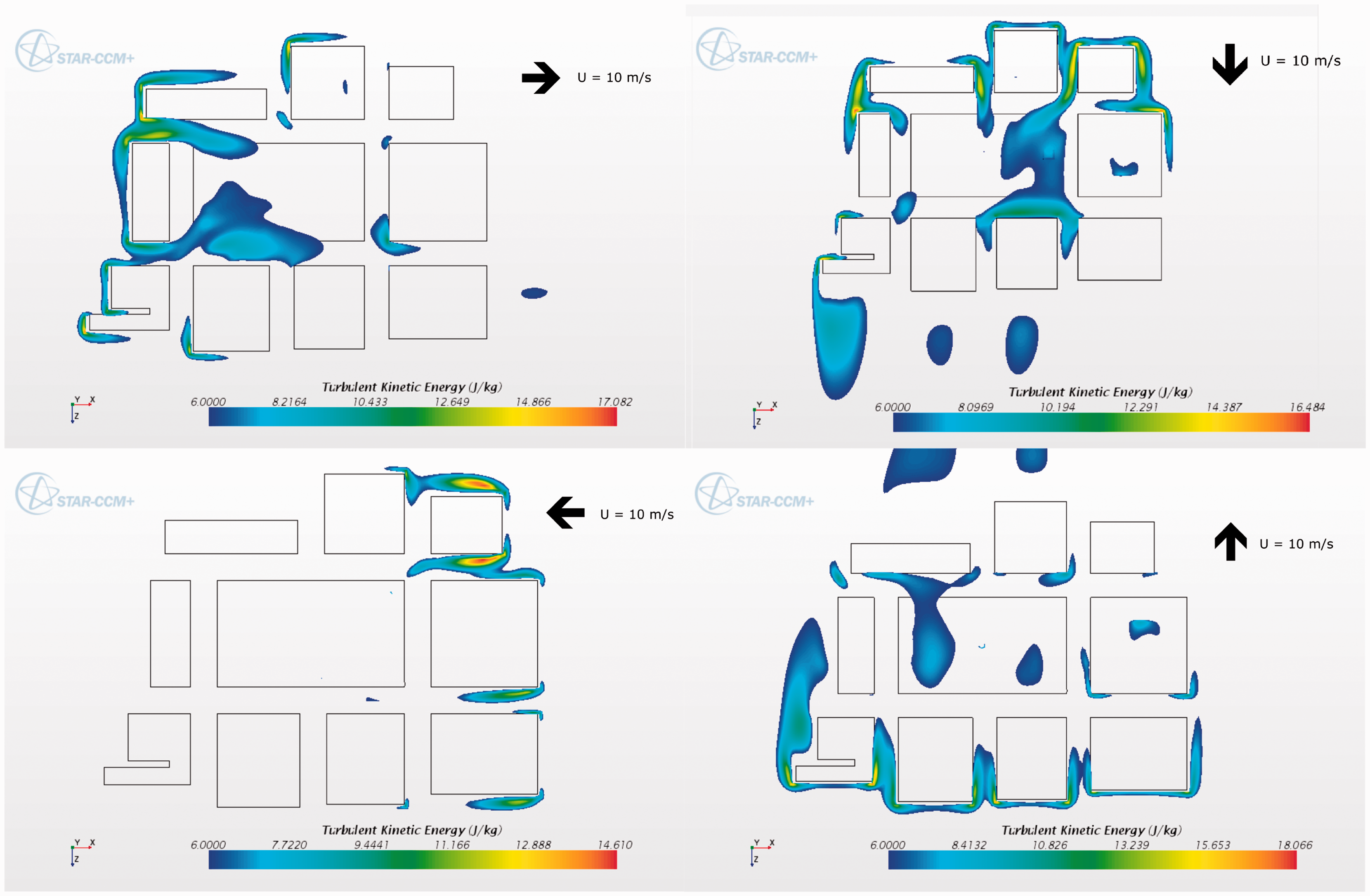

Figure 12 illustrates that given certain wind directions, an environment can be considered to be detrimental to aircraft operations. However, if we analyse the distribution of TKE when the wind is acting in the negative X direction, we see that most of George Square can be inhabited by a small unmanned aircraft. This demonstrates that for identical wind speeds, the prevailing direction could have a great impact on the suitability of a certain area when it comes to UAV operations. Of course, we have only studied four wind directions. The wind could be coming from any direction and shift at any time throughout the day.

Infrastructure development

We have demonstrated that a small unmanned aircraft cannot operate in a congested area without any consideration given to aerodynamic interactions. If we allow these vehicles to operate without a proper understanding of the distribution of turbulence in an urban environment, it could only be determined as either reckless or negligent and damage to persons or property is a very possible outcome. To integrate small unmanned aircraft within this environment, we must amass a data bank which contains numerical results of fluid flow throughout a city for a wide range of weather conditions. As these vehicles are limited in the amount of data that they can store onboard, an infrastructure which allows the free exchange of this data should be developed.

One such method may be to issue daily flight conditions which determine periods of operation within a congested environment when all small unmanned aircraft are grounded. This is a broad approach which presents the simplest solution to this particular problem. However, for commercial UAVs, such a broad approach may represent an undesirable drop in productivity. Similarly, for law enforcement aircraft, it could represent a decrease in effective policing. These are a few of many examples of applications that would be impacted by employing this method.

Another method may be to have all aircraft operate as part of a large, wireless network. Adopting this approach, aircraft could respond instantaneously to changes in environmental conditions and make path planning or other operational decisions immediately. This online method, along with a suitable traffic management system, would maximise the amount of time that aircraft could spend in the air, only withdrawing from the environment completely under extreme conditions.

Any proposed method would also depend on the physical characteristics and control system of each unmanned aircraft. These impact the critical TKE value which determines the conditions that are most detrimental to autonomous aircraft flight. This means that less robust vehicles might spend more time on the ground than their more capable counterparts. This highlights the immediate need to increase focus in the area of disturbance rejection for small unmanned aircraft. The greater the ability an individual vehicle has to withstand the impact of turbulence, the less of a concern the spatially distributed turbulent regions in congested areas become.

Conclusion

With the increased availability and application of UAV technology, the requirement to understand the myriad of environments that we expect aircraft to operate in becomes unavoidable. If small unmanned aircraft are to be utilised in any capacity within a congested area, it is imperative that we understand the flow characteristics in such an environment and quantify their impact on the flight trajectory of the aircraft. Attempting to operate aircraft with no consideration of the aerodynamic effects of building-induced turbulence would result in a detrimental drop in performance. As such, progression towards a future where these vehicles are integrated within an urban airspace is hindered by the lack of reliable data.

Utilising Star-CCM+, we have demonstrated that the spatial distribution of critical TKE is dependent on conditions such as: operating altitude; wind speed and prevailing wind direction. With regard to operating altitude, it was found that flying as low as possible helps to mitigate the impact of turbulence acting on small unmanned aircraft.

CFD results also indicated that when entering an urban environment, descent from the free stream and through the canopy layer is ill advised due to the relationship between altitude and increased turbulence. Thus, as a result of the similarity of flow characteristics, regardless of wind speed, the areas where turbulence is consistently minimised can act as an access point for UAVs. Furthermore, the extent of spatially distributed regions of critical TKE was found to be dependent on the prevailing wind direction. If knowledge of the turbulence within an environment can be combined with real time monitoring of changes in wind direction, paths through a potentially hazardous environment may become feasible. Such a proposal would require the development of an infrastructure which allows communication of changing weather conditions to vehicles from data centres that contain banks of CFD data. This would allow aircraft to make informed decisions on changes in route and whether or not it may be necessary to temporarily ground a vehicle.

However we approach this problem, one thing is certain if we are to integrate UAVs within urban environments: consideration of the building induced aerodynamics and how it impacts vehicle performance must be made. With an increased understanding of how to safely operate in any number of conditions, we can begin to move towards loosening the regulations which currently impede our ability to effectively utilise UAV technology for civil and commercial benefit.

Footnotes

Declaration of conflicting interests

The author(s) declared no potential conflicts of interest with respect to the research, authorship, and/or publication of this article.

Funding

The author(s) disclosed receipt of the following financial support for the research, authorship and/or publication of this article: Funded by the Engineering and Physical Sciences Research Council (EPSRC).

Appendix

References

Civil Aviation Authority. CAP 393: air navigation: the order and the regulations. Version 4.1, April 2015.

Civil Aviation Authority. CAP 722: unmanned aircraft system operations in UK airspace – guidance, 6th ed. UK: Directorate of Airspace Policy, 2015.

Sutherland M and Etele J. Urban wind field generation using LES for application to quadrotor flight. In: Proceedings of the 29th congress of the international council of the aeronautical sciences, St. Petersburg, Russia, 7–12 September 2014.

Salim

Buccolieri

Chan

et al.

Numerical simulation of atmospheric pollutant dispersion in an urban street canyon: comparison between RANS and LES. J Wind Eng Ind Aerodyn 2011; 99: 103–113.

Tominaga

Stathopoulos

. Numerical simulation of dispersion around an isolated cubic building: model evaluation of RANS and LES. Build Environ 2010; 45: 2231–2239.

Sini

. Pollutant dispersion and thermal effects in urban street canyons. Atmos Environ 1996; 30: 2659–2677.

Murray CWA and Anderson D. 3D route planning in a turbulent urban environment. In: AUVSI’s unmanned systems conference, GA, USA, 4–7 May 2015.

Kittiyoungkun S. Aerodynamic problems of urban UAV operations. Internal Report. Department of Engineering and Applied Science, Cranfield University, Cranfield, UK, 2010.

Ohba

. Experimental Study of effects of separation distance between twin high-rise tower models on gaseous diffusion behind the downward tower model. Wind Eng Ind Aerodyn 1998; 77–78: 555–566.

10.

Blocken

Carmeliet

. Pedestrian wind environment around buildings: literature review and practical examples. Build Phys 2004; 28: 107–159.

11.

Oke

. Street design and urban canopy layer climate. Energy Build 1988; 11: 103–113.

12.

Murray CWA, Ireland M and Anderson D. On the response of an autonomous quadrotor operating in a turbulent urban environment. In: AUVSI’s unmanned systems conference, FL, USA, 12–15 May 2014.

13.

Franke J, Hellsten A, Schlünzen H, et al. Best practice guideline for the CFD simulation of flows in the urban environment. COST Action 732, 1 May 2007. Belgium: COST Office.

14.

Blocken

Carmeliet

. Validation of CFD simulations of wind-driven rain on a low-rise building facade. Build Environ 2007; 42: 2530–2548.

15.

Meroney

Leitl

Rafailidis

et al.

Wind-tunnel and numerical modeling of flow and dispersion about several building shapes. J Wind Eng Ind Aerodyn 1999; 81: 333–345.

16.

Tominaga

Stathopoulos

. CFD simulation of near-field pollutant dispersion in the urban environment: a review of current modeling techniques. Atmos Environ 2013; 79: 716–730.

17.

Tominaga Y and Stathopoulos T. Numerical simulation of dispersion around an isolated cubic building: comparison of various types of

k - ɛ

models. Atmos Environ 2009; 43: 3200–3210.

18.

Xie

Castro

. Large-eddy simulation for flow and dispersion in urban streets. Atmos Environ 2009; 43: 2174–2185.

19.

Gousseau

Blocken

van Heijst

GJF

. CFD simulation of pollutant dispersion around isolated buildings: on the role of convective and turbulent mass fluxes in the prediction accuracy. J Hazard Mater 2011; 194: 422–434.

20.

Ireland M and Anderson D. Development of navigation algorithms for nap-of-the-earth UAV flight in a constrained urban environment. In: Proceedings of the 28th congress of the international council of the aeronautical sciences, Brisbane, Australia, 23–28 September 2012.

21.

Ireland M. Investigations in multi-resolution modelling of the quadrotor micro-air vehicle. PhD Thesis, University of Glasgow, Glasgow, UK, 2014.

22.

Leishman

. Principles of helicopter aerodynamics, 2nd ed. Cambridge, UK: Cambridge University Press, 2006.

23.

Fay G. Derivation of the aerodynamic forces for the mesicopter simulation. Unpublished Report. Stanford University, Stanford, CA. 2001.

24.

Brandt JB and Selig MS. Propeller performance data at low Reynolds numbers. In: 49th AIAA aerospace sciences meeting, Orlando, FL, USA, 4–7 January 2011.

25.

Carvalho I. Low Reynolds propellers for increased quadcopters endurance. Master’s Thesis, University of Beira Interior, Portugal, 2013.

26.

Morgado

Silvestre

Páscoa

. Validation of new formulations for propeller analysis. J Propulsion Power 2014; 31: 467–477.

27.

Hoblit

. Gust loads on aircraft: concepts and applications, Washington DC, USA: AIAA Education Series, 1988.

28.

Bagiev

Thomson

Anderson

et al.

Predictive inverse simulation of helicopters in aggressive manoeuvring flight. Aeronaut J 2012; 1175: 87–98.

29.

Hall

Anderson

. Reactive route selection from pre-calculated trajectories – application to UAV path planning. Aeronaut J 2011; 115: 635–640.

30.

McGookin M, Anderson D and McGookin EW. Application of MPC and sliding mode control to IFAC benchmark models. In: Proceedings of the UKACC international conference on control, Manchester, UK, 2–4 September, 2008.

A CFD-based procedure for airspace integration of small unmanned aircraft within congested areas

Abstract

Keywords

Introduction

Environmental modelling

Representation of urban environment

Meshing

Vehicle dynamics

Rigid body dynamics

Rotor inflow model

Modelling of the propeller aerodynamics

Statistical modelling of the temporal variation of velocity components

Performance of quadrotor under the influence of atmospheric turbulence

Quadrotor control

Position control

Attitude control

Generic environment vs. existing cityscape

Results

Variation in TKE with height

Entry points and aerodynamic similarities

Impact of wind direction on spatial distribution of critical turbulence regions

Infrastructure development

Conclusion

Footnotes

Declaration of conflicting interests

Funding

Appendix

References