Development of a low-order model of turbulent non-premixed flame global blow-off

Abstract

A novel model for the global extinction of recirculating non-premixed flames has been developed and validated. This model is based on the imperfectly stirred reactor approach, derived from the spatially integrated conditional moment closure equation, and enhanced with a stochastic model for the scalar dissipation rate, the key characteristics of which can be inferred from computational fluid dynamics data or experimental measurements. We refer to this new model as the stochastic imperfectly stirred reactor. The model’s output is the probability of extinction, which corresponds to the proportion of a flame’s stoichiometric isosurface experiencing local extinctions. A review of the literature suggests that for a flame to blow off globally, about 30% of the stoichiometric isosurface must be extinguished. This criterion was tested against two atmospheric Cambridge swirl spray flame experiments using ethanol and kerosene as fuels. Time-averaged computational fluid dynamics data for these experiments, at conditions far from blow-off, allowed for a calculation of the blow-off velocity within 13% of the experimental values. The stochastic imperfectly stirred reactor model can in principle predict a combustor’s complete blow-off curve with only a limited number of computational fluid dynamics solutions which can be obtained even without a finite-rate turbulent combustion model, as long as the mixture fraction field is reasonably well captured.

Introduction

Understanding the global blow-off (BO) behaviour of a gas turbine combustor is crucial for characterising engine operability. BO, also known as global extinction, refers to the inability of a flame to stabilise, with stability here used loosely as a term to describe either the range of air/fuel ratios (AFRs) where stable combustion can occur or as a measure of the maximum velocities a combustor can tolerate. ¹ If a sufficient number of stable and unstable conditions are known, they can be translated into the operational envelope of the combustor. Stability performance thus informs combustor design from inception to optimisation. Typically, aviation combustion systems operate in non-premixed modes with liquid fuel injections and swirling airflows, leading to complex mixing, heat transfer, and BO behaviour. In new combustor development, however, BO behaviour is rarely predicted, and no empirical correlations or computationally inexpensive numerical methods currently exist that can confidently associate BO with a particular design or geometry change, such as the fuel injector, combustor liner port positions, or the heat shield. Stability assessments thus rely on physical experiments at specific inlet conditions. The ‘lean blow-off’ (LBO) point is identified by gradually reducing fuel flow until flame extinction, repeated across air mass flows to capture stable and unstable regions. LBO points define the stability limit under high AFR conditions, important for reducing pollutants.

Computational fluid dynamics (CFD) simulations may be employed to predict stability limits and the LBO curve, but developing a practical numerical approach for gas turbine combustors is challenging. Physically, extinction occurs due to excessive heat loss or radical depletion, with turbulent non-premixed flames adding complexity due to strong turbulence-mixing-chemistry interactions. Predicting turbulent flame extinction dynamics is actually one of the most important performance measures of turbulent combustion models, with varying success achieved to date primarily through large eddy simulation (LES). ² Most studies, however, focus on localised extinction in lab-scale flames (e.g. see Giusti and Mastorakos, ³ Mohaddes et al. ⁴ and Zhang and Mastorakos^5,6), such as the Sandia jet, ⁷ the Sydney swirl flame,^8,9 and the Cambridge swirling flames,^10,11 rather than full LBO characterisation. Zhang and Mastorakos ⁵ notably used conditional moment closure (CMC) coupled with LES to evaluate the full LBO curve of a swirling non-premixed flame, achieving 25% accuracy in BO limits and duration trends. However, similar works are rare in the combustion CFD literature, and high computational demands continue to hinder practical applications. As a result, developing methods with lower computational cost are needed so as to explore more geometries and operating conditions during the design process.

If one were to predict the LBO curve with CFD, one would need to perform a very large number of simulations, each one of which would have to include a very detailed modelling approach and hence would be a prohibitively expensive design methodology, given that it would have to be used for a range of geometries and operating conditions. This article presents a novel approach that can accelerate this process by reducing the number of necessary computationally intensive reacting CFD and is able to provide a fast and reasonably accurate prediction of BO. The model is based on a stochastic variant of the imperfectly stirred reactor (ISR) approach, ¹² hereafter referred to as the stochastic imperfectly stirred reactor (sISR) method. The sISR method can allow the prediction of a complete LBO curve of a burner with only a limited number of CFD solutions that could in principle be performed even without a finite-rate turbulent combustion model, as long as the mixture fraction field is captured reasonably well. The approach is here developed and evaluated against atmospheric lab-scale recirculating flames using ethanol or kerosene as fuel, and the overall philosophy of this modelling framework is discussed.

The article is organised as follows. First, an overview of the phenomenology of extinction in laminar and turbulent flames is provided based on a short review of the literature. The lessons learnt are then used to develop a numerical model that leverages the sISR method. The model development and all details regarding the coupling of sISR with CFD are summarised next, followed by a demonstration of the approach and its validation against the atmospheric Cambridge swirl spray burner for which blow-off experimental and reference CFD data are available. Conclusions and recommendations for future work close the article.

Phenomenology of extinction

Early studies by Spalding and Jain ¹³ and Liñán ¹⁴ established that in laminar non-premixed flames, if fuel and air mass flow rates exceed a critical strain rate, chemical reactions cease and the flame extinguishes. In such flames, combustion relies on molecular mixing, often expressed as the scalar dissipation rate (SDR), defined as $N\equiv D\mathrm{\nabla }\xi \mathrm{\nabla }\xi$ , where $D$ is the diffusivity of the mixture fraction $\xi$ (ranging from 0 in the oxidiser to 1 in the fuel). Extinction occurs when SDR reaches a critical value $N_{\mathrm{ext}}$ , depending on thermodynamic and chemical properties alone, independent of flow configuration.

Peters and Williams ¹⁵ extended this to turbulent flames, viewing them as laminar flamelets stretched and contorted by the turbulent flow and affected by stochastic variations in SDR. They proposed that when the stoichiometric SDR, $N_{\mathrm{st}}\equiv (N|\xi ={\xi }_{\mathrm{st}})$ , exceeds a critical extinction threshold $N_{\mathrm{st},\mathrm{ext}}$ , ‘holes’ form along the flame sheet. If too many holes develop, the flame sheet continuity is lost, causing local extinction. The probability of sheet continuity, $p_{\mathrm{cont}}\equiv P(N_{\mathrm{st}}\le N_{\mathrm{st},\mathrm{ext}})$ , is linked to flame stability, with the flame extinguishing when this probability drops below a critical level that is about $p_{\mathrm{cr},\mathrm{cont}}=60\mathrm{\%}-70\mathrm{\%}$ . Alternatively, we can think of the critical level being $p_{\mathrm{cr}}\equiv 1-p_{\mathrm{cr},\mathrm{cont}}=30\mathrm{\%}-40\mathrm{\%}$ for the probabilistic distribution of holes in the flame: $p\equiv P(N_{\mathrm{st}}>N_{\mathrm{st},\mathrm{ext}})$ . This probabilistic approach, inspired by continuum percolation theory, can be applied to gas turbine flames to understand BO and we will use it in the remainder of this article. Global extinction, or BO, can be seen as a cumulative effect of local extinctions, weakening flame structure and altering local mixing until the entire flame extinguishes. ¹⁶

The approach by Peters and Williams ¹⁵ assumes a quasi-steady view of extinction, which has limitations. Extinction is not an instantaneous process; it unfolds over time, with ongoing chemical reactions creating ‘memory’ effects, such as radical buildup in laminar flames ¹⁷ and stability in turbulent flames even when SDR surpasses the quasi-steady $N_{\mathrm{ext}}$ . ¹⁸ Additionally, extinction can result from other factors, such as heat losses and droplet interactions that deplete heat or fuel. Localised extinctions can also transiently reduce SDR below $N_{\mathrm{ext}}$ , potentially allowing re-ignition, though ignition and extinction dynamics differ. ¹⁹ Heat and radical transport from nearby hot regions can further stabilise the flame despite exceeding $N_{\mathrm{ext}}$ . Despite its limitations, however, the critical continuity probability $p_{\mathrm{cr},\mathrm{cont}}$ by Peters and Williams ¹⁵ is supported by several studies on turbulent flame structure and stability. For example, the Sandia piloted jet flame experiments ⁷ and related simulations (e.g. see Ihme and Pitsch ²⁰ and Wandel and Lindstedt ²¹ ) analyse local extinction using the burning index (BI) by Xu and Pope. ²² BI, defined as $Y_{(|\xi )}/Y_r$ with $Y_{(|\xi )}$ denoting the first moment of the conditional probability density function (PDF) of a selected scalar and $Y_r$ as a reference peak value in a strained counterflow laminar flame, characterises the degree of local extinction. In turbulent flames, BI values indicate near-complete burning at higher values and extinction at lower ones. Although BI is not directly equivalent to $p_{\mathrm{cr},\mathrm{cont}}$ (or $p_{\mathrm{cr}}$ ), similarities are observed when examining temperature and key combustion products like ${\mathrm{CO}}_2$ and ${\mathrm{H}}_2$ O. In the Sandia flame experiments, flames near BO show a lower temperature-based BI, with flame F exhibiting BI values around 70%, and species-based BI values around 55%–60%, aligning with the critical threshold $p_{\mathrm{cr},\mathrm{cont}}$ of 60%–70%. Sevault et al.’s measurements on oxy-fuel jet flames further support this threshold, showing that flames close to BO have a burning probability near 68% in the neck region, indicating high likelihood of local extinction above this level. Similarly, LES studies of the Cambridge methane swirl flame by Zhang and Mastorakos analysed BO transients, showing the extinguished fraction of the flame surface area prior to blow-off to be in the 20%–40% range, consistent with the probabilistic distribution of holes in the flame. These examples suggest a near-universal threshold for $p_{\mathrm{cr}}$ at 30%–40% even if the data is based on simplified configurations and fuels.

Model development

After the above review of the literature, it is postulated that 30%–40% of the stoichiometric isosurface must be extinguished for global BO of a non-premixed recirculating flame to occur. Predicting BO thus requires quantifying the portion of the isosurface with local extinctions exceeding $p_{\mathrm{cr}}\approx 30\mathrm{\%}$ . To achieve this and develop a predictive yet computationally inexpensive tool for BO, we here propose a methodology based on a stochastic variant of the ISR approach, which we call sISR. The sISR approach is derived from the spatially integrated CMC equation coupled with detailed chemistry and augmented with a stochastic model for the SDR that goes beyond the quasi-steady state view of extinction by Peters and Williams. ¹⁵ By running several realisations of potential BO scenarios, the sISR model’s output is the probability of complete extinction, $p_{\mathrm{ext}}$ , of the combustor tied to the isosurface of the stoichiometric mixture fraction, which can then be interrogated and compared with $p_{\mathrm{cr}}$ so as to quantify BO propensity. In the current implementation, $p_{\mathrm{ext}}$ is subject to three controlling parameters linked to the SDR and determined from CFD or any knowledge about the SDR behaviour coming from experimental measurements and correlations. As such, the calculation of $p_{\mathrm{ext}}$ can be done a priori and many combustor geometries and/or simulations at different conditions can be interrogated quickly. By extension and by suitable interpolation/extrapolation rules of simple ‘global’ quantities tied to the mixing field, it also possible to predict a complete LBO curve of a burner with only a limited number of CFD solutions that could be performed even without a finite-rate turbulent combustion model, as long as the mixing field is captured reasonably well.

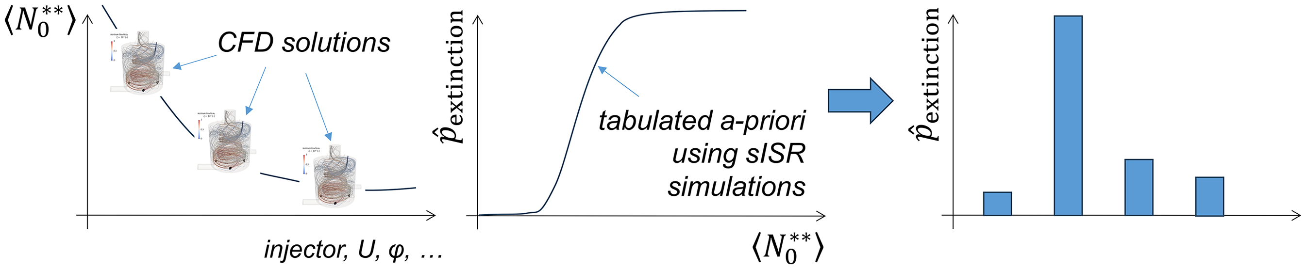
The workflow is summarised in Figure 1. In the following, the sISR simulation methodology will be presented including the governing equation, numerical setup, calculation of $p_{\mathrm{ext}}$ , and the stochastic SDR model, followed by a link to the CFD-derived mixing field and necessary CFD-exported variables.

Figure 1.

Proposed workflow for evaluation BO propensity based on sISR and CFD. Here $⟨N_0^{**}⟩$ refers to a representative time-averaged value of the SDR. BO: blow-off; sISR: stochastic imperfectly stirred reactor; CFD: computational fluid dynamics; SDR: scalar dissipation rate.

Governing equation

The governing equation for an ISR model, based on the singly conditioned CMC method, approximates the full multi-dimensional CMC equation as a zero-dimensional form. ¹² This formulation incorporates the mixture fraction PDF and SDR, extracted from reference CFD simulations with ‘frozen’ flow and mixing fields, allowing ISR to be used as a postprocessor with many chemical mechanisms of arbitrary complexity. In an ISR, conditionally averaged scalars based on the mixture fraction are spatially homogeneous within a volume $V$ here surrounding the stoichiometric flame isosurface. Unlike a perfectly stirred reactor, ISR accommodates mixture fraction inhomogeneities, crucial for analysing local extinction and finite-rate chemistry phenomena. Originally developed by Bilger and co-workers (e.g. see Klimenko and Bilger ¹² and Gkantonas ²³ ), various ISR equations exist, with recent updates by Iavarone et al. ²⁴ and Gkantonas et al. ²⁵

For brevity, the derivation is omitted, but the governing equation is derived from the transport equation of the mass fraction $Q_{\alpha }\equiv Y_{\alpha }|\xi =\eta$ (of species $\alpha$ ) conditioned on the mixture fraction and the mixture fraction PDF, $P_{\eta }$ , with $\eta$ being the sample space variable of the mixture fraction $\xi$ . In the sISR model, a transient term is included as stationarity cannot be assumed. Other key assumptions performed here include (i) differential diffusion is neglected due to the absence of highly diffusive species; (ii) spray evaporation effects are ignored, given their minimal impact near the stoichiometric isosurface; (iii) the model assumes unmixed inlet streams with $P_{\eta }$ at the inlet consisting of two Dirac $\delta$ -functions at $\eta =0$ and $\eta =1$ , reflecting the non-premixed nature of the flames in question.

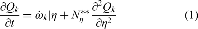
Based on the above the ISR equation becomes a simple transient reaction-diffusion equation given by the following equation:

$$\frac{\mathrm{\partial }{Q}_k}{\mathrm{\partial }t}={\dot{\omega }}_k|\eta +N_{\eta }^{**}\frac{{\mathrm{\partial }}^2{Q}_k}{\mathrm{\partial }{\eta }^2}$$

(1)

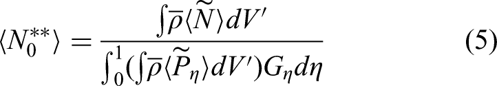
where ${\dot{\omega }}_k|\eta$ is the chemical source term (modelled with first-order closure ¹² ) and $N_{\eta }^{**}$ is the conditional profile of the SDR within the ISR, also known as core-averaged SDR profile. In equation (1), $N_{\eta }^{**}$ is the only variable linked to the mixing field and as such it should reflect the conditions of the flame experienced around the stoichiometric isosurface. Here, we will model $N_{\eta }^{**}$ based on the amplitude mapping closure (AMC) model, ²⁶ as in $N_{\eta }^{**}=N_0^{**}(t)G(\eta )$ , where $G_{\eta }\equiv \exp (-2[{\mathrm{erf}}^{-1}(2\eta -1){]}^2)$ is a prescribed Gaussian-like profile and $N_0^{**}$ a representative SDR that is allowed to fluctuate stochastically. The stochastic variation of $N_0^{**}$ will be explained later.

Numerical Setup

As far as the boundary conditions of equation (1) are concerned, the air temperature and composition must be imposed at the $\eta =0$ boundary and the saturation temperature of the liquid fuel and its composition at the $\eta =1$ boundary. The pressure and enthalpy are assumed constant. Equation (1) is virtually identical to the 0D-CMC equation where the SDR is typically considered to be steady and also using the AMC model. The sISR equation is hence initialised from a 0D-CMC solution with $N_0=⟨N_0^{**}(t)⟩$ . As far as the numerical setup is concerned, an operator splitting technique is implemented following solver choices and discretisation schemes identical to Iavarone et al. ²⁴ Mixture fraction space is discretised into a specified number of nodes (here 76) clustered around the stoichiometric mixture fraction. Here, 76 nodes are used, ensuring adequate resolution of all reacting species and temperature. The total simulation time and number of realisations necessary are discussed in the following.

Probability of extinction

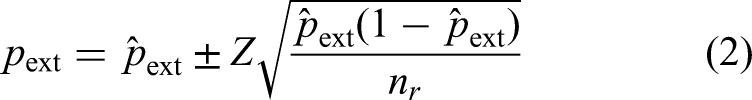
Since $N_0^{**}$ varies stochastically, several realisations of equation (1) are required to find the probability of extinction. If $n_r$ the number of realisations and $n_{\mathrm{ext}}$ the number of realisations where extinction occurs, then $p_{\mathrm{ext}}$ is simply $p_{\mathrm{ext}}=n_{\mathrm{ext}}/n_r$ . The error linked to a finite number of realisations can be estimated from probability theory for binomial trials as in:

$$p_{\mathrm{ext}}={\hat{p}}_{\mathrm{ext}}\pm Z\sqrt{\frac{{\hat{p}}_{\mathrm{ext}}(1-{\hat{p}}_{\mathrm{ext}})}{n_r}}$$

(2)

where ${\hat{p}}_{\mathrm{ext}}$ is the numerical estimate of $p_{\mathrm{ext}}$ and $Z$ is the Z-score for a particular level of confidence. An extinction event is here determined based on the temperature at the stoichiometric mixture fraction, that is, $T_{\mathrm{stoi}}\equiv T|{\eta }_{\mathrm{st}}$ , dropping below a certain threshold which could be, for example, anything in the range 1000–1500 K.

Stochastic scalar dissipation rate model

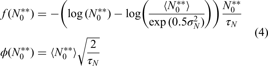
SDR fluctuations, that is, the temporal evolution of $N_0^{**}(t)$ , are modelled using a stochastic differential equation (SDE). Similarly to Pitsch and Fedotov ²⁷ and Gkantonas and Mastorakos, ²⁸ we develop the SDR based on a Stratonovich PDF and a lognormal assumption for the statistics of $N_0^{**}$ . A lognormal assumption for the stationary PDF of the SDR is typical even if experiments and direct numerical simulation (DNS) suggest small but consistent deviations from lognormality at the tails of the distribution. ²⁹ The SDE is given by the following equation:

$$d{N}_0^{**}=f(N_0^{**})dt+{\sigma }_N\varphi (N_0^{**})d{W}_t$$

(3)

where

$$\begin{array}{rl}f(N_0^{**})& =-(\log (N_0^{**})-\log \left(\frac{⟨N_0^{**}⟩}{\exp (0.5{\sigma }_N^2)}\right))\frac{N_0^{**}}{{\tau }_N}\\ \varphi (N_0^{**})& =⟨N_0^{**}⟩\sqrt{\frac{2}{{\tau }_N}}\end{array}$$

(4)

In equations (3) and (4), $d{W}_t$ is a Wiener process, ${\sigma }_N$ is one of the two parameters for the lognormal distribution and ${\tau }_N$ is a characteristic timescale specific to the temporal evolution of the SDR and its autocorrelation time. ${\sigma }_N$ includes contributions from both the mean and the variance of $N_0^{**}$ . Here, it is convenient to link the variance to the mean value by introducing the fluctuation parameter $F=\frac{⟨N_0^{*{*}^{\prime }2}⟩}{⟨N_0^{**}⟩}$ so that ${\sigma }_N=(\log ({\mathit{\text{F}}}^2+1){)}^{0.5}$ . Based on Markides and Chakraborty, ²⁹ we can safely assume that F is approximately the same as its unconditional counterpart for which Sreenivasan ³⁰ has proposed that it scales with $R{e}_{\lambda }^{1/4}$ , with $\lambda$ being the Taylor microscale. Taking into account that $R{e}_{\lambda }\approx \sqrt{(}15R{e}_l)$ with $R{e}_l$ a turbulent Reynolds number, we can consider that $F=(15R{e}_l{)}^{1/8}$ when the SDR fluctuation level is not known from CFD. ${\tau }_N$ induces a ‘memory’ effect to the evolution of $N_0^{**}$ and the various chemical reactions taking place. SDR fluctuations are primarily confined in high wavenumbers of the turbulent spectrum, so based on Gkantonas and Mastorakos ²⁸ and Vedula et al., ³¹ we will consider that ${\tau }_N$ is about 1.6 Kolmogorov timescales, that is, ${\tau }_N\approx 1.6{\tau }_k$ .

Equation (3) is here solved with a Milstein method (see Gkantonas and Mastorakos ²⁸ ) and the total simulation time is taken to be 1 second, which in most cases is O(1000 ${\tau }_N$ ) and provides enough sampling time for the SDE and equation (1) to develop. Multiple realisations are also necessary to calculate the probability of extinction. A maximum limit to the value of $N_0^{**}$ might also be imposed, essentially ‘clipping’ its lognormal distribution. One is a physical limit that is related to the steepest gradient the flame can ever encounter and is given by $N_{\lim }=D/{\lambda }_B^2$ . Another could be a statistical limit, which could be lower or higher than the physical limit, that can be explicitly linked to a given percentile of the distribution, such as the 99.999%-th percentile. Imposing a statistical limit can help avoid very rare events and outliers.

Link to mixing field and usage of CFD

As mentioned previously, three global parameters govern $N_0^{**}(t)$ , and by extension, the sISR model. Among these, the probability of extinction was found to correlate most strongly with the time-averaged value $⟨N_0^{**}⟩$ . Note that $⟨N_0^{**}⟩$ is the only parameter that can singularly alter the probability of extinction from 0% to 100%. It is therefore recommended to prioritise linking $⟨N_0^{**}⟩$ directly to the CFD solution whenever possible. While the remaining parameters, $F$ and ${\tau }_N$ , can also be extracted from CFD data, the reference simulations used here lacked suitable statistical detail. This limitation warrants careful consideration in future studies, including a systematic exploration of all parameters and how they are computed. As a first-order approximation, we instead use global turbulence characteristics, specifically, a representative integral length scale and velocity fluctuation, to estimate a characteristic Reynolds number $R{e}_l$ and a turbulence timescale ${\tau }_k$ for each flame. Based on these, we model $F$ and ${\tau }_N$ as $F=(15R{e}_l{)}^{1/8}$ and ${\tau }_N\approx 1.6{\tau }_k$ , respectively. Given a suitably time-averaged mixing field from an LES simulation (see also Iavarone et al. ²⁴ for a discussion in the context of ISR models), $⟨N_0^{**}⟩$ can then be estimated via:

$$⟨N_0^{**}⟩=\frac{\int \overline{\rho }⟨\tilde{N}⟩d{V}^{\prime }}{{\int }_0^1(\int \overline{\rho }⟨{\tilde{P}}_{\eta }⟩d{V}^{\prime })G_{\eta }d\eta }$$

(5)

where $⟨\widetilde{.}⟩$ denotes the time-averaged value of a LES-filtered (conditional or unconditional) scalar, and the volume integration region is a modelling choice. The volume integration region affects all reference CFD cells and it can be chosen so that a narrow or wide band (volume) around the stoichiometric isosurface is selected. This will be discussed in more detail later.

Although simplified estimates based on global turbulence quantities are used in this study due to limited statistical detail in the available CFD data, we also outline how these parameters may be obtained directly from LES or time-averaged CFD solutions, provided suitable turbulence statistics are available. In the context of LES, the parameter $F$ can be estimated from the variance of the SDR. This is done by performing a volume integration similar to equation (5), substituting $⟨\tilde{N}⟩$ with $\frac{\sqrt{⟨{\tilde{N}}^2⟩-⟨\tilde{N}{⟩}^2}}{⟨\tilde{N}⟩}$ . The parameter ${\tau }_N$ can, in principle, be derived from a mass-weighted integration or estimated from the autocorrelation time of the filtered SDR. However, typical sampling frequencies in LES simulations are often too low to reliably compute the autocorrelation time. As a practical alternative, we propose approximating ${\tau }_N$ using ${\tau }_N\approx 1.6{\tau }_k$ , where ${\tau }_k$ originates from a volume integration step analogous to equation (5), substituting $⟨\tilde{N}⟩$ with $1.6⟨(\nu /\epsilon {)}^{1/2}⟩$ with $\nu$ denoting the kinematic viscosity and $\epsilon$ the instantaneous dissipation rate of turbulent kinetic energy provided by the sub-grid scale model. This approach is not pursued in the present study, but could be implemented if suitable LES statistics are available.

In the context of time-averaged CFD, the same model for ${\tau }_N$ could be applied. For the estimation of $F$ , the local Reynolds number $R{e}_l$ can be approximated from the local turbulent kinetic energy $k$ and dissipation rate $\epsilon$ as $R{e}_l=\frac{k^2}{\nu \epsilon }$ . Furthermore, the mean scalar dissipation rate $⟨N⟩$ can be taken from the turbulence closure model employed for the variance of the mixture fraction around the mean, $\overline{{\xi }^{\prime 2}}$ . For example, under the common assumption that the dissipation rate of scalar fluctuations follows the dissipation of turbulent kinetic energy, one may use $N=\frac{C_d}{2}\frac{\epsilon }{k}\overline{{\xi }^{\prime 2}}$ , where $C_d\approx 2$ is a model constant.

Chemical mechanisms

Two chemical mechanisms are used in this work. As will be explained later, we investigate an ethanol and a kerosene flame. For the first, we consider the skeletal mechanism of Millán-Merino et al. ³² with 34 species and 69 reactions. For the kerosene flame, we consider the mechanism of Nehse et al. ³³ with 39 species and 174 reactions where kerosene is modelled as a single-component surrogate. The critical value above which extinction occurs corresponds to $N_{0,\mathrm{ext}}=443$ s⁻¹ for ethanol and $N_{0,\mathrm{ext}}=584$ s⁻¹ for kerosene. It is important to note that $N_{0,\mathrm{ext}}$ and by extension the probability of extinction depend greatly on the choice of chemical mechanism.

Investigated burner and conditions

The Cambridge swirl spray burner is selected for validation purposes, which consists of a square section enclosure, open to the atmosphere at the outlet and with a hollow-cone pressure atomiser fitted to a conical bluff-body holder. The swirling air flow is supplied through an annular duct surrounding the bluff body, allowing the generation of a swirl-stabilised flame. Experimentally, BO was achieved by operating at constant fuel mass flow rate and increasing the air mass flow rate until the OH* chemiluminescence measurement indicated an extinguished flame. For more details, see Yuan. ¹⁰ Here we investigate (i) an ethanol flame, as characterised experimentally by Yuan ¹⁰ and simulated with LES-CMC by Giusti and Mastorakos, ³ and (ii) a Jet-A (A2) flame, as characterised experimentally by Allison et al. ¹¹ and simulated with LES-CMC by Foale. ³⁴ In the ethanol flame, LBO was observed at case E1B (see Yuan ¹⁰ ) where the bulk velocity $U_b=21.6$ m/s and the fuel mass flow rate is 0.27 g/s (overall equivalence ratio being 0.15), but CFD data for stable case E1S1 with same fuel mass flow rate but bulk velocity 79% of the BO velocity are used here. In the kerosene flame, BO was also recorded at similar bulk velocity and fuel mass flow conditions. Here we focus only on a case with bulk velocity 74% of the BO velocity for which time-averaged CFD data are available. It is important to note that in both flames, stable conditions far from blow-off are only analysed. These are thus used to approximate $p_{\mathrm{ext}}$ at stable conditions and investigate if the BO velocity can be captured by appropriately scaling $⟨N_0^{**}{⟩}_{\mathrm{CFD}}$ . This will be discussed in more detail later.

The LES results available were not sufficient to even crudely approximate parameters the spatial distribution and mass-average values of $F$ and ${\tau }_N$ . Instead, a range of possible values was found based on global turbulence characteristics. Based on the experiments, $u^{\prime }$ is in the order of 20%–40% of the bulk velocity (i.e. in the order of 4–10 m/s) and the integral length scale $l$ is in the order of 1–5 mm, although they depend on space and are most likely anisotropic. This means that $F$ is in the range of 2.5–3.0 and ${\tau }_N$ in the range of 50–100 $\mu$ s in the Cambridge swirl spray burner.

Results and discussion

Stochastic ISR simulations and ‘combustor-agnostic’ BO evaluation

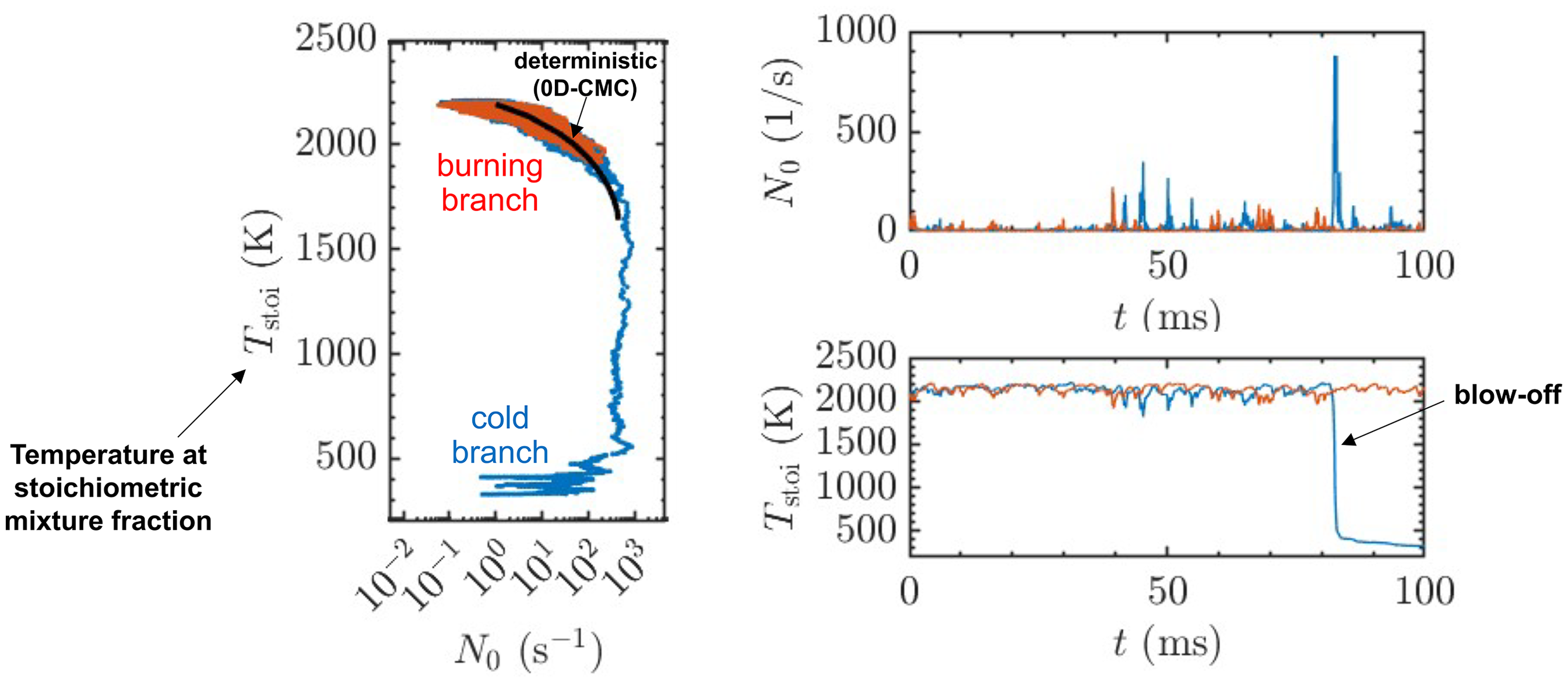
Figure 2 presents two representative sISR simulations of the ethanol atmospheric Cambridge swirl flame. On the right, two realisations are depicted: one fully burning for a duration of 100 ms and another blowing off after 80 ms of simulation. On the left, scatter plots of the corresponding temperature $T_{\mathrm{stoi}}$ and the local SDR are shown. Note that here $N_0^{**}$ is used interchangeably with $N_0$ . It becomes evident that after BO, a transition from the burning to the cold branch occurs. However, the stochastic nature of the SDR and the ensuing fluctuations result in a significant departure from the deterministic curve connecting $T_{\mathrm{stoi}}$ to $N_0$ , which is representative of strained laminar flames. Important differences between the stochastic and deterministic simulations are also apparent in all other reacting scalars, although these are not shown here. Instead, the focus is on the occurrence of BO across multiple realisations and the extraction of $p_{\mathrm{ext}}$ , which represents the proportion of the stoichiometric isosurface experiencing local extinctions.

Figure 2.

Representative stochastic imperfectly stirred reactor (sISR) simulations of the ethanol atmospheric Cambridge swirl flame showing two realisations, one burning and the other blowing off after 80 ms. Note that $N_0^{**}$ is replaced by $N_0$ above.

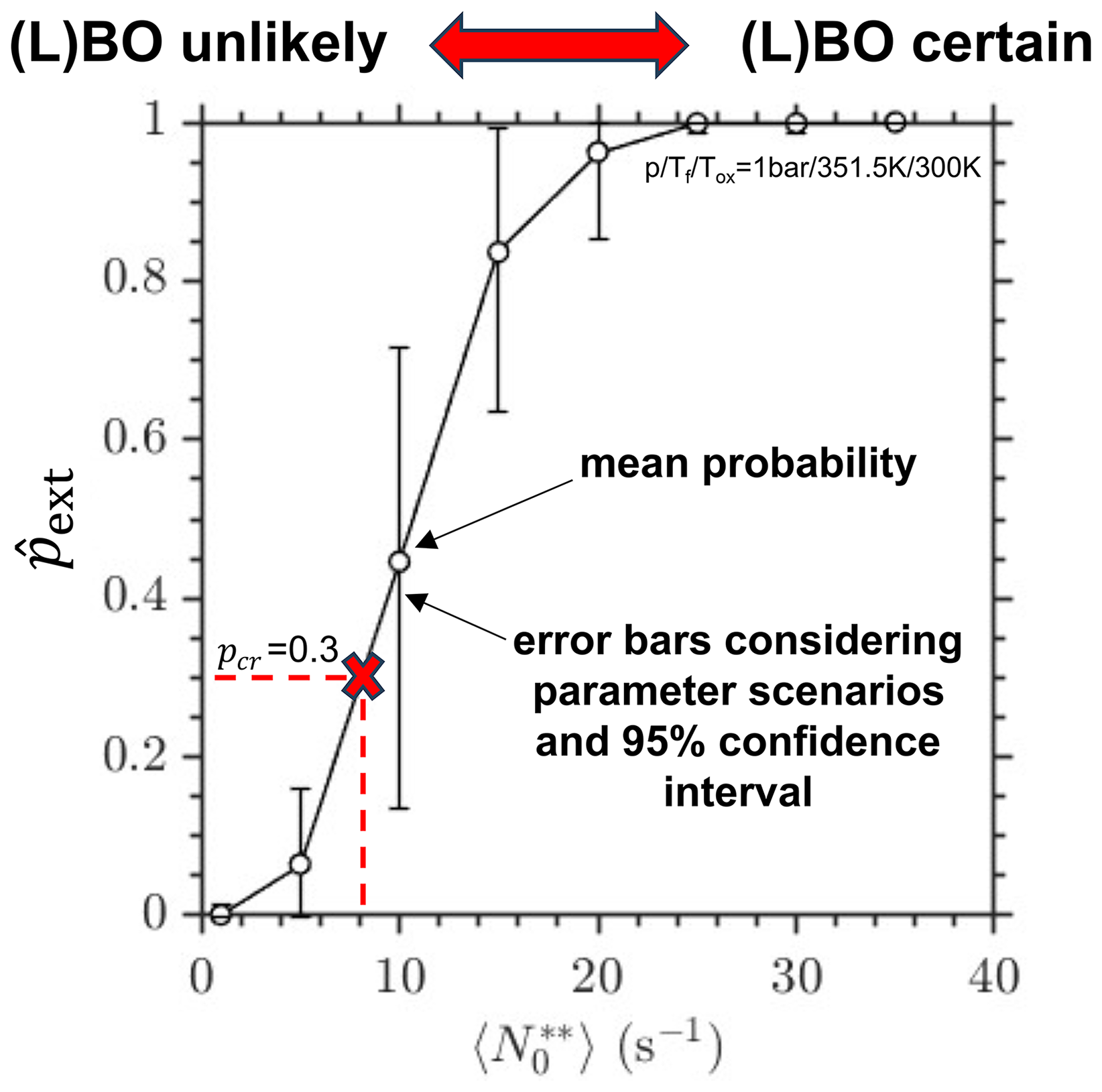
Following the sISR methodology and Figure 1, a ‘map’ for the probability of extinction can be created. This is illustrated in Figure 3 for the ethanol atmospheric Cambridge swirl flame. The black line represents the numerical $p_{\mathrm{ext}}$ estimate ${\hat{p}}_{\mathrm{ext}}$ versus $⟨N_0^{**}⟩$ . ${\hat{p}}_{\mathrm{ext}}$ follows a sigmoid-like function, increasing as $⟨N_0^{**}⟩$ rises. Consequently, as we move towards the right of the curve, the BO propensity increases. If we adopt $p_{\mathrm{cr}}\approx 30\mathrm{\%}$ as a critical threshold, the portion of the plot right and above the red dashed lines can be considered an unstable region where BO becomes certain. In Figure 3, the ${\hat{p}}_{\mathrm{ext}}$ curve and the error bars are derived from four different scenarios for a range of parameters $F$ and ${\tau }_N$ . The scenario-specific ${\hat{p}}_{\mathrm{ext}}$ versus $⟨N_0^{**}⟩$ curves and error bars have much smaller error bars as they are based solely on the binomial trial theory (not shown here). It is important to note, however, that we observe a sensitivity of ${\hat{p}}_{\mathrm{ext}}$ to parameters $F$ and ${\tau }_N$ , with the sensitivity to F being stronger in the investigated range. It is important to explore these sensitivities in greater detail in future studies by considering a broader range of scenarios.

Figure 3.

Numerical estimate of the probability of extinction and respective error based on 200 sISR realisations for the conditions of the ethanol atmospheric Cambridge swirl flame. Here a mean probability and aggregate error are reported from four different scenarios in the $F$ - ${\tau }_N$ space. The critical threshold for LBO, $p_{\mathrm{cr}}$ , is also indicated. sISR: stochastic imperfectly stirred reactor; LBO: lean blow-off.

Similar curves for the probability of extinction can also be created for the kerosene atmospheric Cambridge swirl flame, which are comparable in shape to that of the ethanol flame (not shown here). The evaluation of BO discussed above may be considered partly ‘combustor-agnostic’ as it does not specifically depend on any combustor characteristics apart from the operating conditions used and the pre-selected range for $F$ and ${\tau }_N$ . With a larger database encompassing a wider range of conditions and parameters, this evaluation could become fully combustor-agnostic. The link with the combustor will be established next where $⟨N_0^{**}⟩$ is referenced from the CFD data.

Analysis of CFD data and extrapolation from far-from-BO to near-BO conditions

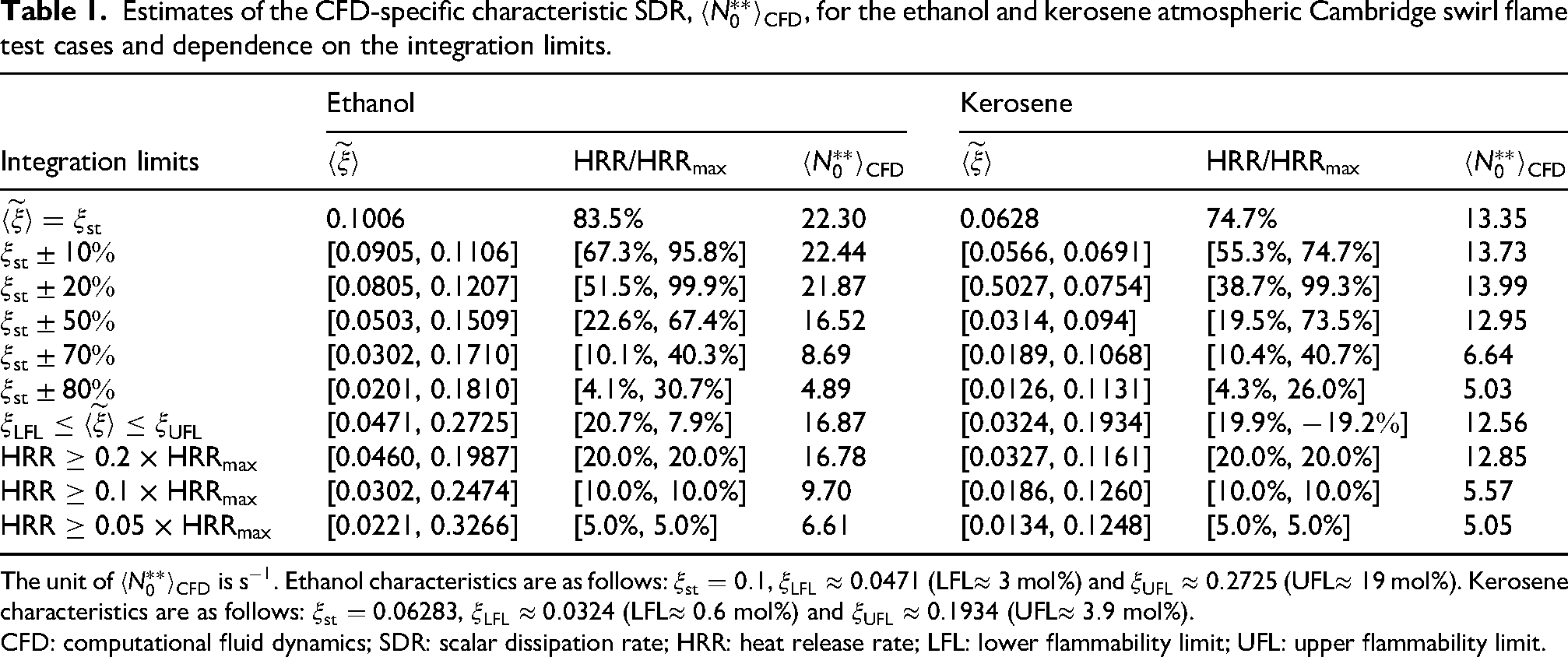
The estimates of $⟨N_0^{**}⟩$ based on the available CFD data are given in Table 1. Several integration limits have been considered when processing the data and in particular, the time-averaged value of the mixture fraction. The integration limits were chosen to be either (i) within pre-determined mixture fraction bands around the stoichiometric mixture fraction, (ii) or within the lower and upper flammability limits (LFL and UFL) of the given fuel-air mixture, or, finally, (iii) within a pre-determined heat release rate (HRR) range determined from a 0D-CMC solution at near-extinction conditions and normalised by the maximum HRR of the same solution. The corresponding mixture fraction and HRR ranges are provided in Table 1.

Table 1.

Estimates of the CFD-specific characteristic SDR, $⟨N_0^{**}{⟩}_{\mathrm{CFD}}$ , for the ethanol and kerosene atmospheric Cambridge swirl flame test cases and dependence on the integration limits.

	Ethanol			Kerosene
Integration limits	$⟨\tilde{\xi }⟩$	HRR/HRR ${}_{\max }$	$⟨N_0^{**}{⟩}_{\mathrm{CFD}}$	$⟨\tilde{\xi }⟩$	HRR/HRR ${}_{\max }$	$⟨N_0^{**}{⟩}_{\mathrm{CFD}}$
$⟨\tilde{\xi }⟩={\xi }_{\mathrm{st}}$	0.1006	83.5%	22.30	0.0628	74.7%	13.35
${\xi }_{\mathrm{st}}\pm 10\mathrm{\%}$	[0.0905, 0.1106]	[67.3%, 95.8%]	22.44	[0.0566, 0.0691]	[55.3%, 74.7%]	13.73
${\xi }_{\mathrm{st}}\pm 20\mathrm{\%}$	[0.0805, 0.1207]	[51.5%, 99.9%]	21.87	[0.5027, 0.0754]	[38.7%, 99.3%]	13.99
${\xi }_{\mathrm{st}}\pm 50\mathrm{\%}$	[0.0503, 0.1509]	[22.6%, 67.4%]	16.52	[0.0314, 0.094]	[19.5%, 73.5%]	12.95
${\xi }_{\mathrm{st}}\pm 70\mathrm{\%}$	[0.0302, 0.1710]	[10.1%, 40.3%]	8.69	[0.0189, 0.1068]	[10.4%, 40.7%]	6.64
${\xi }_{\mathrm{st}}\pm 80\mathrm{\%}$	[0.0201, 0.1810]	[4.1%, 30.7%]	4.89	[0.0126, 0.1131]	[4.3%, 26.0%]	5.03
${\xi }_{\mathrm{LFL}}\le ⟨\tilde{\xi }⟩\le {\xi }_{\mathrm{UFL}}$	[0.0471, 0.2725]	[20.7%, 7.9%]	16.87	[0.0324, 0.1934]	[19.9%, $-19.2\mathrm{\%}$ ]	12.56
HRR $\ge$ 0.2 $\times$ HRR ${}_{\max }$	[0.0460, 0.1987]	[20.0%, 20.0%]	16.78	[0.0327, 0.1161]	[20.0%, 20.0%]	12.85
HRR $\ge$ 0.1 $\times$ HRR ${}_{\max }$	[0.0302, 0.2474]	[10.0%, 10.0%]	9.70	[0.0186, 0.1260]	[10.0%, 10.0%]	5.57
HRR $\ge$ 0.05 $\times$ HRR ${}_{\max }$	[0.0221, 0.3266]	[5.0%, 5.0%]	6.61	[0.0134, 0.1248]	[5.0%, 5.0%]	5.05

The unit of $⟨N_0^{**}{⟩}_{\mathrm{CFD}}$ is s⁻¹. Ethanol characteristics are as follows: ${\xi }_{\mathrm{st}}=0.1$ , ${\xi }_{\mathrm{LFL}}\approx 0.0471$ (LFL $\approx 3$ mol%) and ${\xi }_{\mathrm{UFL}}\approx 0.2725$ (UFL $\approx 19$ mol%). Kerosene characteristics are as follows: ${\xi }_{\mathrm{st}}=0.06283$ , ${\xi }_{\mathrm{LFL}}\approx 0.0324$ (LFL $\approx 0.6$ mol%) and ${\xi }_{\mathrm{UFL}}\approx 0.1934$ (UFL $\approx 3.9$ mol%).

CFD: computational fluid dynamics; SDR: scalar dissipation rate; HRR: heat release rate; LFL: lower flammability limit; UFL: upper flammability limit.

As shown in Table 1, the resulting value of $⟨N_0^{**}⟩$ is sensitive to the choice of integration limits and shows a general decreasing trend as the integration limits widen. This is expected as a larger volume is considered and the aggregate SDR (and by extension, the effect of micromixing) becomes smaller. Out of the various integration limits, some have a more physical interpretation and will be discussed in more detail later. The dependence of $F$ and ${\tau }_N$ to the integration limits could not be examined here due to the lack of appropriate data but a significant sensitivity is similarly expected.

The CFD data used and the $⟨N_0^{**}⟩$ values presented in Table 1 are at conditions far from BO. The question then arises as to how we can predict the mixing field and the respective value of $⟨N_0^{**}⟩$ (and the rest of parameters) at conditions near to BO. Here, we will use a simple scaling law that connects the residence time of the burner/combustor to $⟨N_0^{**}⟩$ and allows us to extrapolate from smaller to higher bulk velocities.

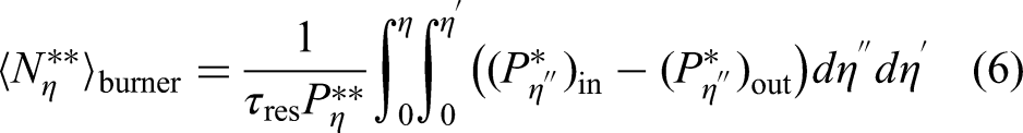
As discussed by Klimenko and Bilger, ¹² the volume weighted conditional SDR of any control volume, $⟨N_{\eta }^{**}⟩$ , can be found based on the double integration of the mixture fraction’s PDF transport equation to give as follows:

$$⟨N_{\eta }^{**}{⟩}_{\mathrm{burner}}=\frac{1}{{\tau }_{\mathrm{res}}{P}_{\eta }^{**}}{\int }_0^{\eta }{\int }_0^{{\eta }^{{}^{\prime }}}((P_{{\eta }^{{}^{″}}}^{*}{)}_{\mathrm{in}}-(P_{{\eta }^{{}^{″}}}^{*}{)}_{\mathrm{out}})d{\eta }^{{}^{″}}d{\eta }^{{}^{\prime }}$$

(6)

where ${\tau }_{\mathrm{res}}$ is the burner residence time and $P_{\eta }^{**}$ is the PDF of the mixture fraction at the inlet or outlet of the burner. If we ignore the effect of the mixture fraction PDFs to the shape and magnitude of $⟨(N_{\eta }^{**}⟩{)}_{\mathrm{burner}}$ when changing conditions, $⟨(N_{\eta }^{**}⟩{)}_{\mathrm{burner}}$ is inversely proportional to ${\tau }_{\mathrm{res}}$ which in turn is inversely proportional to the total mass flow running through the burner/combustor. As a first-order approximation, we can therefore link $⟨N_0^{**}⟩$ directly to the total mass flow since $⟨N_0^{**}⟩$ is a characteristic value tied to $⟨(N_{\eta }^{**}⟩{)}_{\mathrm{burner}}$ and the AMC model selected for the conditional SDR around the stoichiometric isosurface of the flame. If $⟨(N_{\eta }^{**}⟩{)}_{\mathrm{burner}}$ increases, the SDR field of the whole burner, including around the stoichiometric isosurface of the flame, should increase proportionally.

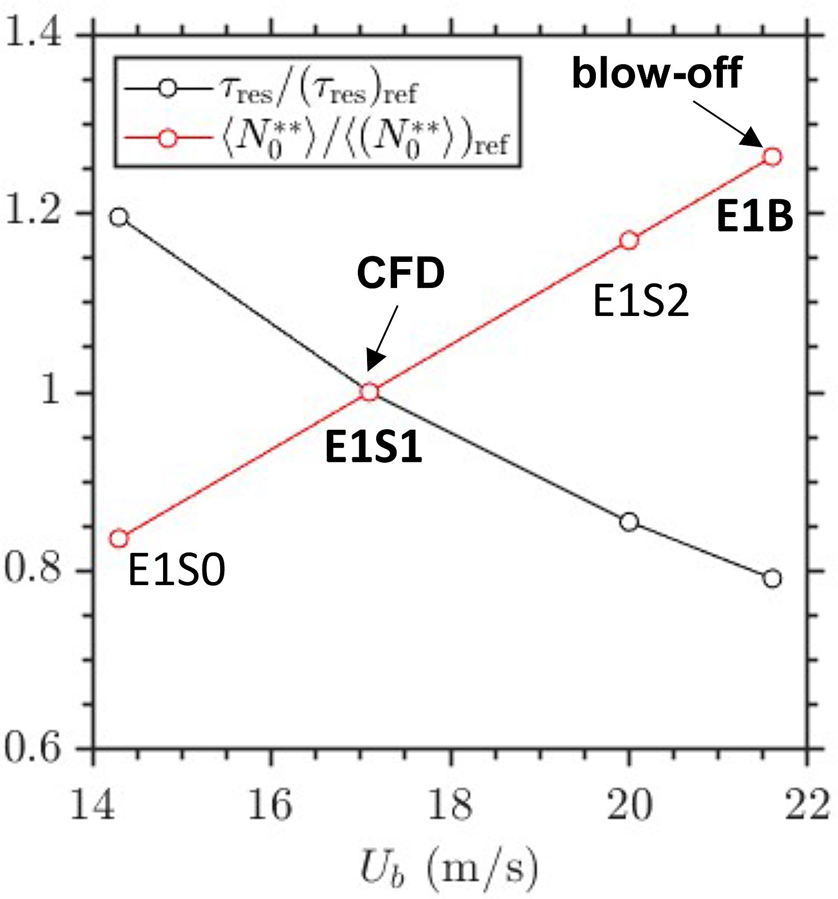
For constant fuel mass flow, it turns out that $⟨N_0^{**}⟩\propto U_b$ as the bulk velocity is directly proportional to the total mass flow. Using one CFD solution as an ‘anchor’ (reference), this allows us to scale $⟨N_0^{**}⟩$ with a simple linear relationship as shown in Figure 4. For the ethanol case, $⟨N_0^{**}⟩$ at BO conditions should be 1/0.79 $\approx$ 1.26 higher than the reference since $U_b/U_{\mathrm{BO},\exp }=79\mathrm{\%}$ . For the kerosene case, $⟨N_0^{**}⟩$ at BO conditions should be 1/0.74 $\approx$ 1.35 higher than the reference.

Figure 4.

Change of burner residence time with bulk velocity $U_b$ and simple linear relationship between $U_b$ and $⟨N_0^{**}⟩$ . Data are based on the ethanol atmospheric Cambridge swirl spray burner test cases. The reference is case E1S1 and the blow-off (BO) case is E1B.

Predicted BO velocity and comparison with experiment

Provided (i) the extraction of $⟨N_0^{**}⟩$ from the CFD data, (ii) the simple scaling rule to extrapolate from far-from-blow-off to near-blow-off conditions and (iii) the ‘combustor-agnostic’ numerical estimates of the $p_{\mathrm{ext}}$ , it becomes possible to predict the BO velocity of each test case. The procedure is outlined as follows:

Select the most suitable integration limits from Table 1 and extract the characteristic $⟨N_0^{**}{⟩}_{\mathrm{CFD}}$ (and parameters $F$ and ${\tau }_N$ where applicable) from the CFD data.

Create an interpolant for ${\hat{p}}_{\mathrm{ext}}$ (e.g. using linear interpolation) and determine the $p_{\mathrm{ext}}$ value corresponding to the CFD data.

Using the interpolant of Step 2 to find the parameter values (here $⟨N_0^{**}⟩$ ) at BO conditions, corresponding to ${\hat{p}}_{\mathrm{ext}}=p_{\mathrm{cr}}$ .

Use the scaling based on the residence time and the proportionality between bulk velocity and SDR to extrapolate and find the equivalent bulk velocity at the BO conditions of Step 3, $U_{\mathrm{BO},\mathrm{sim}}$ , using the data from Step 1.

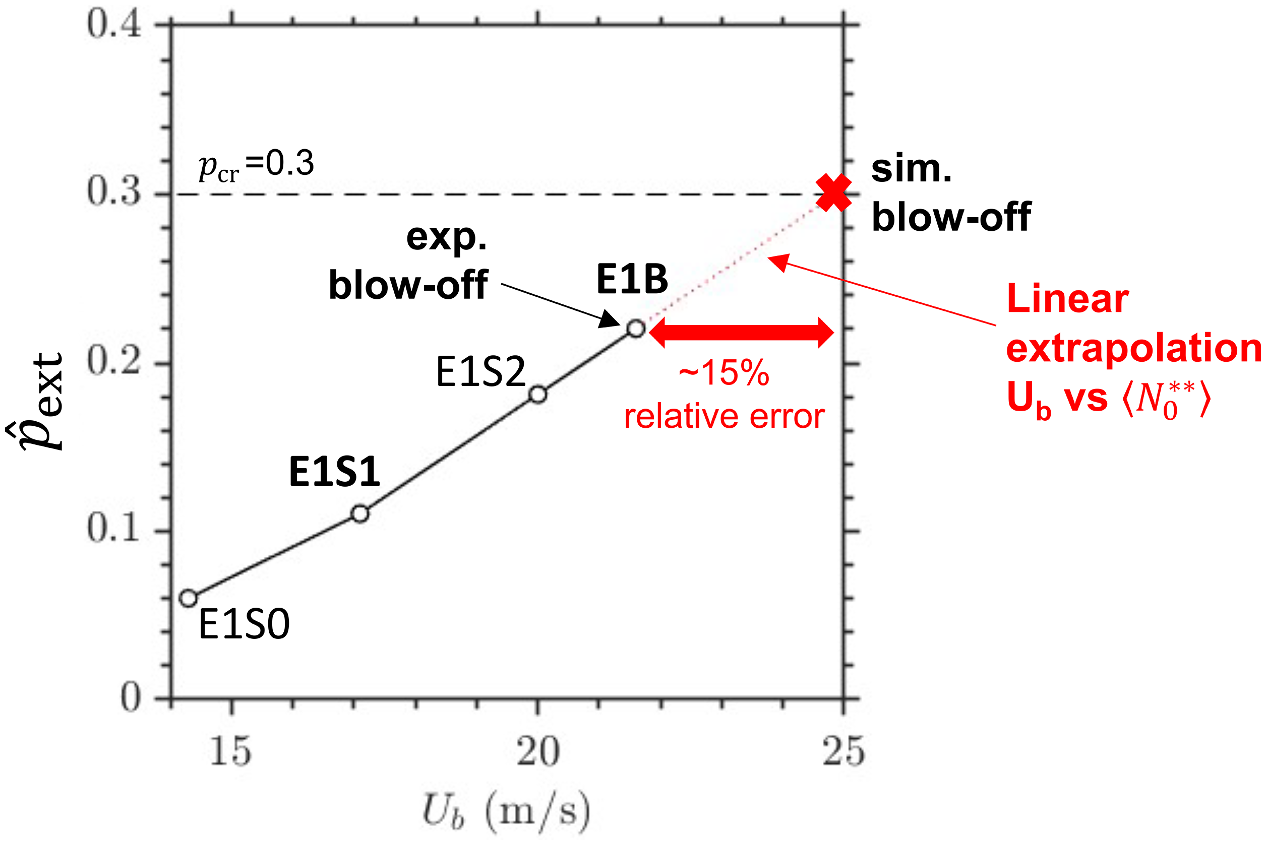
Figure 5 provides a representative example of this procedure for the ethanol atmospheric Cambridge swirl flame. The relative error between $U_{\mathrm{BO},\mathrm{sim}}$ and the experimental BO velocity is $\sim$ 15%, with $U_{\mathrm{BO},\mathrm{sim}}$ being overpredicted. Although the chemical mechanism could play a role, this overprediction occurs because the reference CFD-derived SDR value, $⟨N_0^{**}{⟩}_{\mathrm{CFD}}$ , for case E1S1 is likely underpredicted either due to a misrepresentation of the mixing field or suboptimal integration limits around the stoichiometric isosurface, used for calculating $⟨N_0^{**}{⟩}_{\mathrm{CFD}}$ .

Figure 5.

Application of blow-off velocity prediction procedure to ethanol atmospheric Cambridge swirl flame. Note that this result is not optimal and smaller errors can be achieved with a suitable choice of integration limits for the extraction of $⟨N_0^{**}⟩$ around the stoichiometric isosurface of the flame.

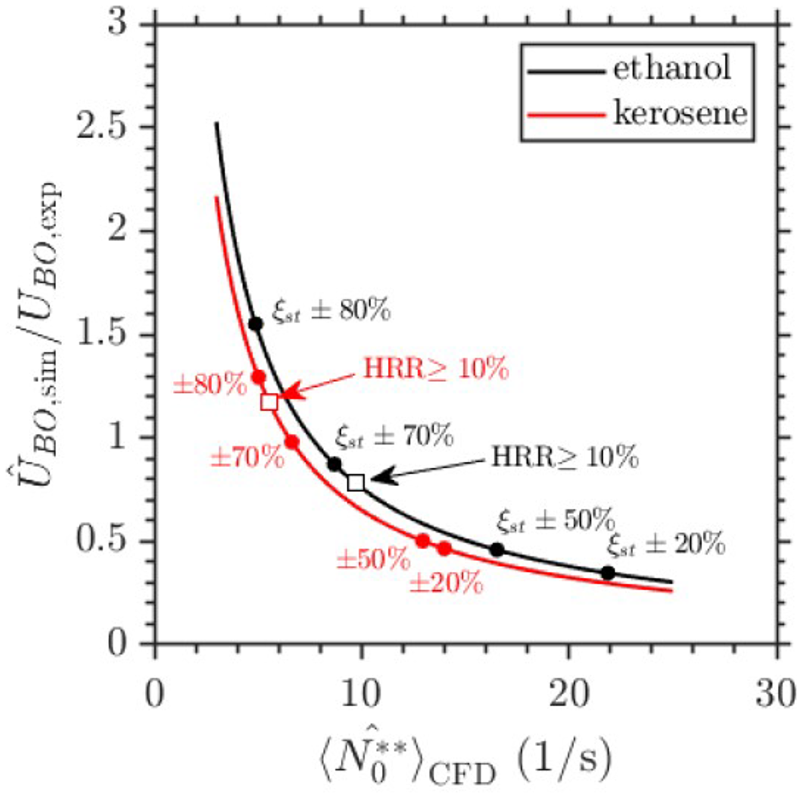
The sensitivity of the results to $⟨N_0^{**}{⟩}_{\mathrm{CFD}}$ can be better appreciated from Figure 6, which shows the ratio of $U_{\mathrm{BO},\mathrm{sim}}$ to the experimental BO velocity as a function of $⟨N_0^{**}{⟩}_{\mathrm{CFD}}$ for both the ethanol and kerosene atmospheric Cambridge swirl flames. The scatter points correspond to selected integration limits of Table 1, while the curves show a wider range of possible $⟨N_0^{**}{⟩}_{\mathrm{CFD}}$ values. A perfect match between experiments and simulations is achieved when $⟨N_0^{**}{⟩}_{\mathrm{CFD}}=7.6$ s⁻¹ for ethanol and 6.5 s⁻¹ for kerosene. Lower (higher) $⟨N_0^{**}{⟩}_{\mathrm{CFD}}$ values result in overprediction (underprediction) of the BO velocity.

Figure 6.

Ratio of predicted blow-off velocity to experimental blow-off velocity of the ethanol and kerosene atmospheric Cambridge swirl flames as a function of the CFD-specific SDR value, $⟨N_0^{**}{⟩}_{\mathrm{CFD}}$ . The scatter points correspond to selected integration limits. CFD: computational fluid dynamics; SDR: scalar dissipation rate.

The closest match for both flames is achieved with integration limits in the range of ${\xi }_{\mathrm{st}}\pm 70\mathrm{\%}$ . For the ethanol flame, this results in $U_{\mathrm{BO},\mathrm{sim}}\approx 0.87U_{\mathrm{BO},\exp }$ , and for the kerosene flame, $U_{\mathrm{BO},\mathrm{sim}}\approx 1.07U_{\mathrm{BO},\exp }$ . This corresponds to relative errors of 12.8% and 6.9%, respectively. It is noteworthy that the ${\xi }_{\mathrm{st}}\pm 70\mathrm{\%}$ limits correspond to $\sim$ 10% and 40% of the peak HRR at the lean and rich limits, respectively (see Table 1). This mixture fraction band contains a large part of the heat release zone but it is not symmetric. Extending the rich limit to 10% of the peak HRR to select a larger part of the heat release zone and achieve a symmetry around the HRR results in a larger underprediction for ethanol and a larger overprediction for kerosene.

Based on the above, we recommend using the integration limits to ‘tune’ the model. The ${\xi }_{\mathrm{st}}\pm 70\mathrm{\%}$ integration limits achieve the highest accuracy for both flames with a relative error of $\le 13\mathrm{\%}$ . Since $p_{\mathrm{cr}}=30\mathrm{\%}$ and the selected integration limits can be matched to any $p_{\mathrm{cr}}$ , the rule of thumb $p_{\mathrm{cr}}+X=1$ arises, where $X=70\mathrm{\%}$ in this context.

Conclusions

We introduce a novel low-order methodology for predicting the global extinction of recirculating non-premixed flames. This approach estimates the extinction probability, $p_{\mathrm{ext}}$ , representing the fraction of a flame’s stoichiometric isosurface undergoing local extinctions, and imposes a critical limit on $p_{\mathrm{ext}}$ to predict BO occurrence. The methodology uniquely combines a stochastic variant of the ISR model, termed the sISR model, with SDR characteristics extracted from time-averaged CFD data and a scaling approach from far-from-BO to near-BO conditions. Applied to two atmospheric Cambridge swirl spray flame experiments with ethanol and kerosene, the sISR model predicted BO velocities within 13% of experimental values by using a residence-time-based SDR scaling and estimating SDR fluctuations and timescales from global turbulence characteristics inferred by the experiments. Accurate predictions required setting integration limits around the stoichiometric isosurface to identify a representative SDR in the reference CFD data, with optimal limits found at ${\xi }_{\mathrm{st}}\pm 70\mathrm{\%}$ for a $p_{\mathrm{ext}}$ BO threshold of 30%. The significance of this model lies in its capability for rapid, accurate BO predictions using minimal CFD input, potentially without advanced finite-rate turbulent combustion models, thus enabling efficient exploration of combustor designs and conditions. Future work will expand this methodology to realistic combustors, enhance CFD data use to establish generally applicable guidelines for model ‘tuning’, and develop a comprehensive BO curve.