Combustion dynamics analysis of a pressurized airblast swirl burner using proper orthogonal decomposition

Abstract

Jet fuel-fired combustors in aero gas turbine engines have switched to lean burn to decrease nitric oxide emissions in recent years as a result of strict emission regulations. Lean operating conditions, however, exhibit a heightened sensitivity to thermoacoustic instabilities and such burners require careful consideration in design and operation. Similar to natural gas-fired combustors, they exhibit thermoacoustic instabilities, but the characteristics are more complex and less well-studied. This paper presents a numerical investigation of an airblast jet fuel swirl burner operating with preheated air at lean pressurized conditions. In order to understand the acoustic characteristics of the in-house designed burner (Magister UT burner), detached eddy simulations are performed at relevant aero engine conditions. Simulation results are then analyzed by means of our internally developed parallel modal analysis package, PARAMOUNT, to perform proper orthogonal decomposition (POD) on large datasets. The resulting modes are inspected to highlight flow features of interest and their associated acoustic frequencies at unforced conditions. Single frequency acoustic forcing is employed to study the acoustic response of the burner to perturbations at similar frequencies to its precessing vortex core. We show that parallel computation of POD modes is a viable tool to investigate the main flow features of swirl burners and is suitable for highlighting the important acoustic frequencies without the need to employ fully compressible computational fluid dynamics solvers. Additionally, the analysis method reveals the ways in which various flow structures correlate with each other and how external perturbations modify them.

Introduction

The ever more relevant concerns surrounding global climate change and pollutant emissions have long been the driving force in the design of gas turbine engines. ¹ Major advances in the field of aero gas turbine engine design including aerodynamics, combustion, cooling, and materials have been shaped by these concerns as well. ² These engines have to meet a long list of operational safety standards as well as environmental requirements which can bring about conflicting design goals and further complicate the design process.

An important hallmark of modern jet engine design has been the focus on combustion emissions such as unburnt hydrocarbons, carbon monoxide (CO), soot formation, and nitrogen oxides (NOx). Rich Quench Lean (RQL) operation mode has been a well-understood and widely used combustion technology that has successfully improved jet engine emissions.^3,4 As manufacturers continue to improve fuel efficiency and emission levels, low-emission combustion schemes become more desirable. Lean premixed pre-vaporized combustion (LPP) is one such combustion approach that is fundamentally different from the established RQL technology but comes with its own set of concerns and design challenges. ⁵

One of the major concerns in employing LPP technology in aero engines is the susceptibility of this combustion mode to thermoacoustic instabilities.^6,7 These instabilities arise as a feedback loop between oscillatory flow and perturbations in the heat release rate (HRR) of the flame. Provided that the HRR and acoustic pressures are sufficiently in-phase in order to satisfy the Rayleigh criterion, the instabilities can grow stronger and compromise the engine. ⁸

Thermoacoustic instabilities are challenging to resolve as they often occur having reached higher technology readiness levels where making design modification is more costly and prohibitive. ⁹ Aero engines often utilize swirling flows which can improve fuel-oxidizer mixing, enhance flame anchoring within the combustion chamber ¹⁰ and provide the basis for pre-filming airblast fuel atomization commonly studied and used in aero engines. ¹¹ The acoustically compact nature of the flame, however, can further complicate the concerns regarding thermoacoustic instabilities in such burners. The challenge is to predict this at an early design stage by means of computational fluid dynamics (CFD) simulations. ¹²

Large eddy simulation (LES) remains one of the most effective and popular numerical methodologies to investigate swirl-stabilized burners. Performing reliable LES of turbulent combustion phenomena, however, remains a significant undertaking that demands considerable computational resources and generates large amounts of data. The analysis of LES results has garnered significant attention in recent years with emphasis on investigating flow patterns within similar swirl burners in a variety of configurations using proper orthogonal decomposition (POD).^13–15 These exemplary investigations, however, typically focus on premixed combustion and highlight some difficulties and limitations of this approach. Firstly, performing POD on such LES results requires significant computational resources and manual intervention to consider many variables within the flow field that might be relevant to the investigation. Secondly, the interpretation of POD mode shapes requires expert domain knowledge and is largely a qualitative and subjective process. Finally, the secondary interplay between POD modes and across multiple variables and operating conditions is normally not considered.

Motivated by the challenges of thermoacoustic instabilities in LPP aero engine designs, this paper focuses on the analysis of combustion dynamics using POD inside an aero engine representative swirl burner under partially premixed conditions. To this end, the Magister UT Burner is an airblast pre-filming swirl burner designed at the University of Twente. It utilizes liquid jet fuel and operates with preheated air to 473 K at pressurized conditions. Coupled with its compact flame, it has been designed to study thermoacoustic instabilities at conditions characteristic of aero engines. We shall discuss this further in section “Burner Design.”

In order to analyze the combustion dynamics, detached eddy simulations (DESs) have been conducted by means of a weakly compressible flow solver to obtain a highly resolute simulation of the combustion phenomena in both space and time. In this approach, a Reynolds averaged Navier–Stokes (RANS) model is employed in regions of the flow with lower turbulence, while a LES model is used in regions with significant turbulence which in turn, enables an accurate prediction of the flow field while maintaining computational efficiency.

Preliminary cold flow experimental analysis of the burner conducted in our laboratory at the University of Twente hinted at the presence of a precessing vortex core (PVC) which is a coherent vortical structure that rotates around the burner axis and has a single or double helical structure. The PVC has been observed in both reacting and non-reacting or cold flows in swirl-stabilized combustors^16–18 and it has great implications on their performance due to having an effect on turbulent mixing and thermoacoustic characteristics. The precession frequency of the PVC in similar swirl-stabilized combustors has been shown to be highly sensitive to inlet air velocity and the gradient of rotational velocity and located in the inner shear layer of the vortex breakdown region.^19,20 While in most cases, the combustion phenomena have been shown to suppress the PVC, ²¹ it has been demonstrated that in some cases, the PVC frequency does not change between hot and cold flows. ²²

The experimentally observed PVC frequency was compared to the numerically predicted value to assess the validity of cold flow simulations. Additionally, liquid droplet injection experiments were conducted at Karlsruhe Institute of Technology (KIT) and used to further validate the cold flow simulation results as well as to find a suitable droplet distribution for the combustion simulations. The setup for numerical simulation of liquid fuel combustion and comparison with measurements are discussed in section “Liquid fuel measurements.”

The combustion simulation results were then analyzed by means of our in-house modal analysis software package called PARAMOUNT. This package was developed with the aim of facilitating modal analysis of large datasets such as DES and provide tools to inspect the relationship between POD modes and other variables of interest. The analysis employs a parallel computation approach to obtain a decomposition for flow variables of interest. We discuss this in section “POD formulation in PARAMOUNT.”

In our analysis, the POD results were inspected to infer combustion dynamics using the power spectral density (PSD) of POD mode coefficients as well as the associated POD mode shapes. The frequencies of interest were analyzed to understand their origin and provide insight into the burner combustion instabilities. A correlation methodology is introduced to cast light on how the multitude of modes across all considered variables correlate with each other and with other volume-integrated variables. Furthermore, the same methodology was applied to the result of a separate DES computation subject to acoustic forcing at the air inlet. A comparison between the POD analysis of the two simulations reveals the ways in which forcing modifies certain mode shapes and how external forcing manifests itself in terms of a change in various mode shapes. These findings are detailed in section “Results and Discussion,” followed by our concluding remarks.

Burner design

Magister UT Burner was designed with the aim of studying thermoacoustic instabilities in aero engines. It provides a relatively compact flame in a lean partially premixed setup within the combustion chamber while keeping the pressure drop across the burner at a minimum. The burner consists of three main components that fit together to form the flow passages as seen in Figure 1.

Figure 1.

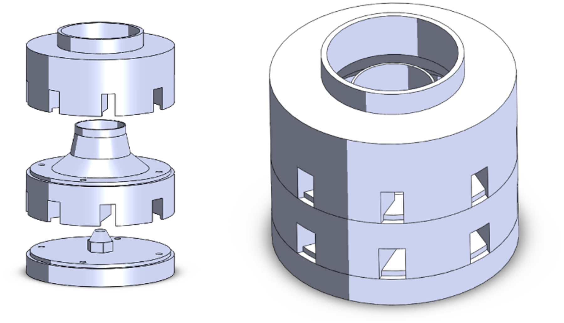
Overview of the Magister UT Burner components and geometry.

The burner directs the combustion air into two distinct sets of entry channels that each consists of eight ducts. The primary and secondary airflow through the two channels and meet each other further inside the burner to create a region of high shear force due to the significant velocity difference between the two. The design schematic can be seen in Figure 2 depicting primary air entry ducts labeled “A” and the secondary entry ducts labeled “B.” Liquid fuel is injected at the base of the burner by means of a hollow cone nozzle. Here the smaller droplets get entrained in the primary air flow but the bulk of the combustion fuel forms a thin wall on the inside of the burner. The fuel film travels further downstream into the shear region where it is further atomized in an airblast fashion.

Figure 2.

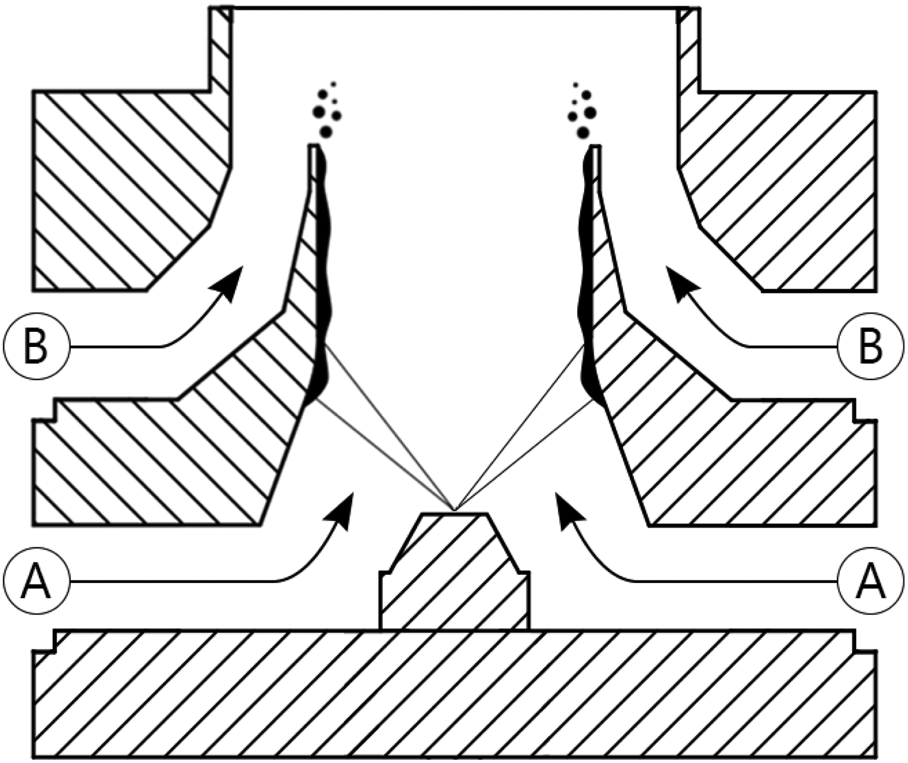
Magister UT Burner schematic.

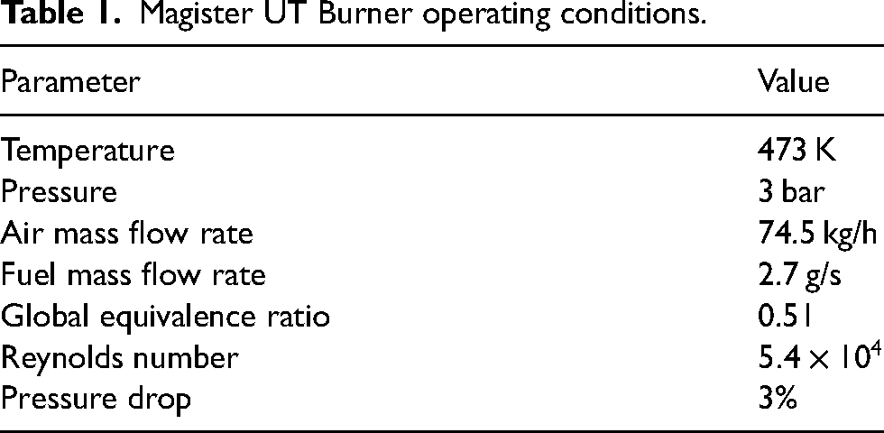
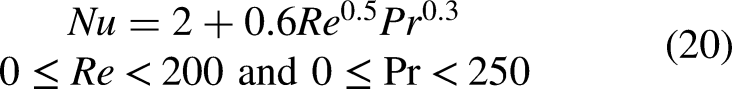
The operating conditions of the burner are summarized in Table 1. These conditions induce a swirl number of 1.2 in the flow and result in an exhaust temperature of around 1700 K and a power delivery of around 82 kW per bar (250 kW in total) while maintaining a low-pressure drop of around 3% suitable for thermoacoustic studies and representative for aero-engine combustors. The fuel selection is interchangeable between diesel and Jet-A fuel. For the purposes of this study, diesel is used as a liquid fuel.

Table 1.

Magister UT Burner operating conditions.

Parameter	Value
Temperature	473 K
Pressure	3 bar
Air mass flow rate	74.5 kg/h
Fuel mass flow rate	2.7 g/s
Global equivalence ratio	0.51
Reynolds number	$5.4\times {10}^4$
Pressure drop	3%

Numerical setup

The CFD approach employs Lagrangian tracking of the fuel droplets while the turbulent combusting flow is described in an Eulerian manner. To that end, the numerical grid is prepared by means of a semi-structured voxel methodology better suited for particle tracking. ²³ The three-dimensional (3D) mesh consists of roughly 20 million elements and includes the combustion chamber as well as an upstream casing in which the swirler is situated. The cross-section view of the burner mesh near the dump plane can be seen in Figure 3. Special attention has been paid to the shear region of droplet breakup and near-wall inflation layers to ensure proper resolution for the wall-bounded LES analysis. Orthogonal advancing-front surface meshing algorithm with an inflation layer growth rate of 1.2 results in a higher quality mesh with better boundary features. ²⁴ Stream-wise element elongation coupled with a slight chamber contraction is employed near the outlet boundary to prevent unwanted reflections and recirculation zones. ²⁵

Figure 3.

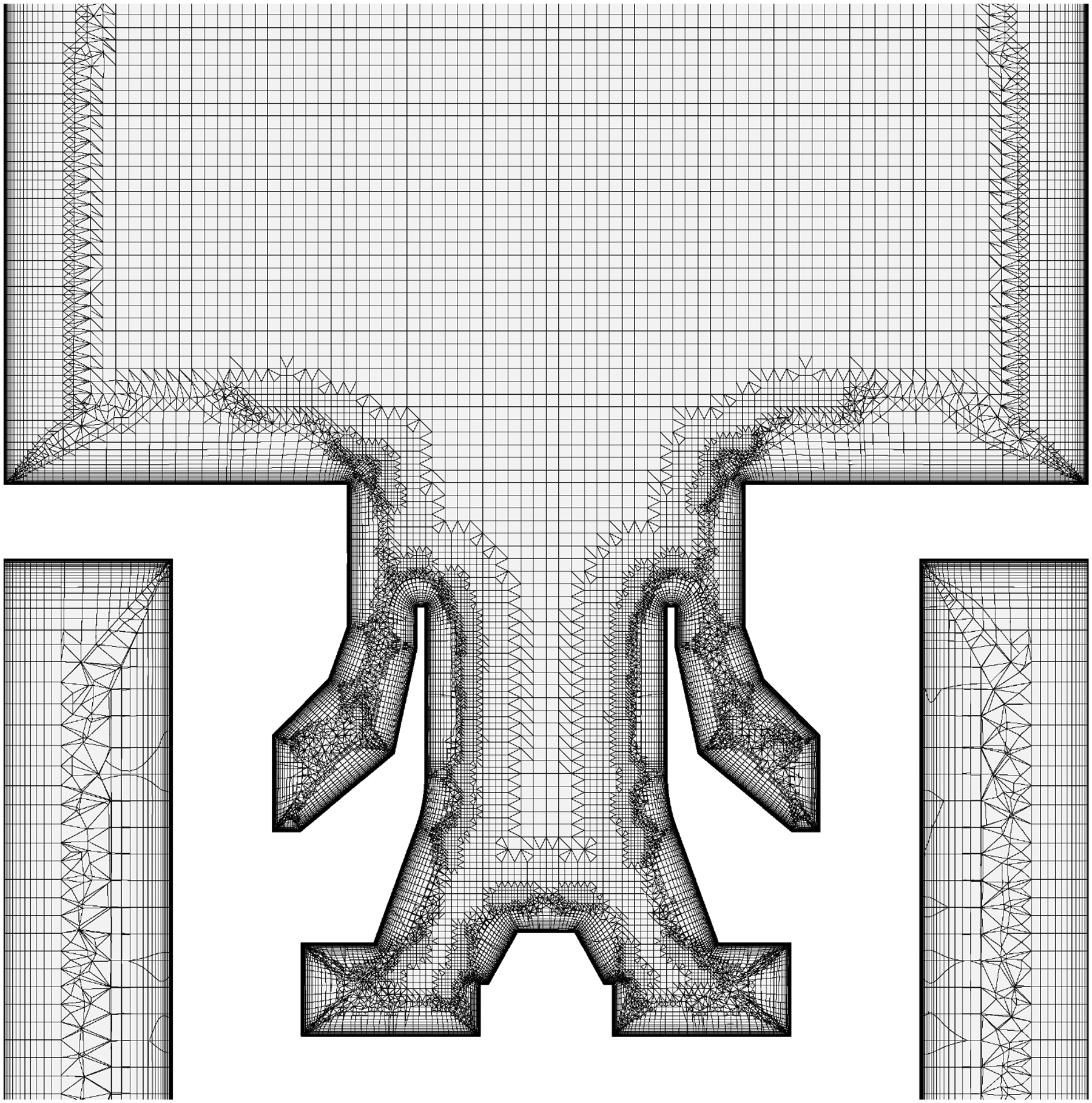
Cross-section view of the adopted voxel meshing scheme.

DES is then performed using flow analysis software Ansys CFX v19.2. In this framework, the wall boundary layer region is computed by the RANS model and the free shear flows away from walls are computed in LES mode. The handover between the two models is determined by means of a blending function limiter that compares the maximum edge length of the computational cell to the characteristic length computed based on local turbulence levels. The relevant equations for all the models used in this study are available in CFX documentations. 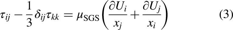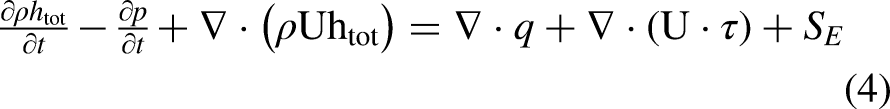²⁶ Here we highlight the governing equations for the LES model that is used to compute the bulk of the reactive flow.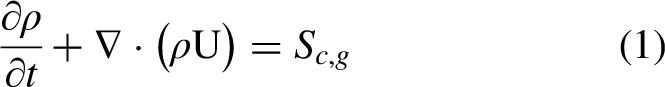

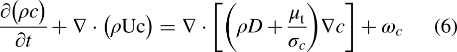
$$\frac{\mathrm{\partial }\rho }{\mathrm{\partial }t}+\mathrm{\nabla }\cdot \left(\rho \text{U}\right)=S_{c,g}$$

(1)

$$\frac{\mathrm{\partial }(\rho \text{U})}{\mathrm{\partial }t}+\mathrm{\nabla }\cdot (\rho \text{U}\times \text{U})=-\mathrm{\nabla }\rho +\mathrm{\nabla }\cdot \tau +S_{M,g}$$

(2)

$${\tau }_{ij}-\frac{1}{3}{\delta }_{ij}{\tau }_{kk}={\mu }_{\mathrm{SGS}}(\frac{\mathrm{\partial }{U}_i}{x_j}+\frac{\mathrm{\partial }{U}_j}{x_i})$$

(3)

$$\begin{array}{cc}& \frac{\mathrm{\partial }\rho h_{\mathrm{tot}}}{\mathrm{\partial }t}-\frac{\mathrm{\partial }p}{\mathrm{\partial }t}+\mathrm{\nabla }\cdot \left(\rho \text{U}{h}_{\mathrm{tot}}\right)=\mathrm{\nabla }\cdot q+\mathrm{\nabla }\cdot (\text{U}\cdot \tau )+S_E\end{array}$$

(4)

The solver uses a non-staggered grid with a second-order resolution for advection terms and turbulence modeling for the gaseous phase which solves the conservative form of the continuity equation detailed in equation (1). Here, $\rho$ refers to the mixture averaged density, $\text{U}$ refers to the LES filtered velocity vector, and $S_{c,g}$ denotes the source term in the gaseous phase. The mass source term in the liquid phase $S_{c,l}$ is discussed later in equation (21). Other notable and relevant governing equations for the LES of a filtered low Mach number reactive flow regime include the conservation of momentum and the conservation of energy equations shown in equations (2) and (4). Here, $S_M$ denotes the momentum source term. The large-scale turbulent flow is solved directly and the influence of the small scales is taken into account by $\tau$ which refers to the sub-grid scale (SGS) stress following an eddy-viscosity approach shown in equation (3). ${\mu }_{\mathrm{SGS}}$ represents the SGS viscosity and is calculated by means of the Smagorinsky formulation based on gradients of the filtered velocity using the Smagorinsky constant value of $0.1$ . $h_{\mathrm{tot}}$ refers to the total enthalpy of the flow, $q$ refers to the heat transfer from the flow and $S_E$ refers to the energy equation source term. For details on momentum and energy source terms, we refer the reader to CFX documentation guide. ²⁶

In view of the demanding computational resources needed to describe the combustion processes in detail, a simplified approach is adopted to describe the evolution of the turbulent reactive mixture using a reaction progress variable (RPV) as defined in equation (5) with 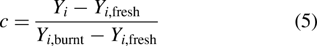$Y_{\mathrm{fresh}}$ referring to the mass fraction in the non-reacted fraction of the fluid and $Y_{\mathrm{burnt}}$ the species mass fraction in the burnt fractions. This variable is computed by solving the transport equation (6), where the turbulent Schmidt number for RPV is ${\sigma }_c$ =0.9. The source term ${\omega }_c$ in this equation is formulated using the burning velocity model (BVM) as seen in equation (7), where ${\rho }_{\mathrm{u}}$ is the density of the unburnt mixture and $\rho D$ referring to the mixture dynamic diffusivity. The closure term $S_{\mathrm{T}}$ ²⁷ is presented in equation (8) with the leading factor $A=0.5$ , turbulent velocity fluctuating component $u^{\prime }$ , laminar burning velocity $S_L$ , thermal conductivity of unburnt mixture ${\lambda }_{\mathrm{u}}$ , and integral turbulent length scale $l_{\mathrm{t}}$ . The dominant swirl present in the flow can cause a considerable amount of flame stretch and a careful selection of flame stretch factor $G$ is necessary to account for reduced flame velocity as a result of a large dissipation rate of turbulent kinetic energy. In CFX, $G$ is determined by means of an error function and empirical model coefficients. Here, a value of 10,000  ${\mathrm{s}}^{-1}$ was adopted in accordance with numerical simulations of similar combustors. ²⁸

$$c=\frac{Y_i-Y_{i,\mathrm{fresh}}}{Y_{i,\mathrm{burnt}}-Y_{i,\mathrm{fresh}}}$$

(5)

$$\frac{\mathrm{\partial }\left(\rho c\right)}{\mathrm{\partial }t}+\mathrm{\nabla }\cdot \left(\rho \text{U}c\right)=\mathrm{\nabla }\cdot \left[(\rho D+\frac{{\mu }_{\mathrm{t}}}{{\sigma }_c})\mathrm{\nabla }c\right]+{\omega }_c$$

(6)

$${\omega }_c={\rho }_{\mathrm{u}}{S}_{\mathrm{T}}|\mathrm{\nabla }c|-\mathrm{\nabla }\cdot (\rho D\mathrm{\nabla }\cdot c)$$

(7)

$$S_{\mathrm{T}}=AG{u^{\prime }}^{3/4}{s}_L^{1/2}{\lambda }_{\mathrm{u}}^{-1/4}{l}_{\mathrm{t}}^{1/4}$$

(8)

In addition to the BVM model used to describe the progress of the global reaction, a laminar flamelet-generated manifold library with a presumed probability density function (beta-PDF) with a unity Lewis number assumption $(L{e}_i=1)$ is used to determine the composition of the reacted and non-reacted fractions of the fluid. In this methodology, a library is used to tabulate mean species mass fractions $Y_i$ based on mean mixture fraction $Z$ , its fluctuation $Z^{″}$ and a scalar dissipation rate $\mathcal{X}$ as shown in equations (9) and (10):

$$Y_i=(1-c)Y_{i,\mathrm{fresh}}+c{Y}_i^{\mathrm{flamelet}}$$

(9)

$$Y_i^{\mathrm{flamelet}}=Y_i^{\mathrm{flamelet}}(Z,Z^{″},\mathcal{X})$$

(10)

Two additional transport equations are employed to track the evolution of $Z$ and $Z^{″}$ ^28,26 as shown in equations (11) and (12), respectively.

$$\frac{\mathrm{\partial }\left(\rho Z\right)}{\mathrm{\partial }t}+\mathrm{\nabla }\cdot \left(\rho \text{U}Z\right)=\mathrm{\nabla }\cdot \left[(\mu +\frac{{\mu }_{\mathrm{t}}}{{\sigma }_Z})\mathrm{\nabla }Z\right]$$

(11)

$$\begin{array}{c}\frac{\mathrm{\partial }\left(\rho Z^{″2}\right)}{\mathrm{\partial }t}+\mathrm{\nabla }\cdot \left(\rho \text{U}{Z}^{″2}\right)=\mathrm{\nabla }\cdot \left[(\mu +\frac{{\mu }_{\mathrm{t}}}{{\sigma }_{Z^{″2}}})\mathrm{\nabla }{Z}^{″2}\right]+2\frac{{\mu }_{\mathrm{t}}}{{\sigma }_Z}{\left(\mathrm{\nabla }Z\right)}^2-\rho \mathcal{X}\end{array}$$

(12)

Here, the statistical information on the mixture fraction $Z$ is obtained from the mixture fraction variance $Z^{″}$ . The last two terms in equation (12) refer to the production and the dissipation of the mixture fraction variance. The fuel chosen in this study similar to the experimental setup in the University of Twente is diesel. Diesel fuel consists mainly of paraffins, aromatics, and naphthenes. These hydrocarbons typically include between 12 and 20 carbon atoms with boiling temperatures in the range of 443 to 663 K. A possible choice of surrogate for diesel is a blend of trimethyl benzene (nine carbon atoms) and $n$ -dodecane (12 carbon atoms). ²⁹ In this study, $n$ -decane (10 carbon atoms) is chosen as a diesel representative fuel surrogate at the desired operating condition together with the specified laminar burning velocity. The local equivalence ratio is defined based on the mixture fraction as shown in equation (13). A beta function correlation based on maximum burning velocity $S_0^{max}$ and the corresponding equivalence ratio ${\phi }_{max}$ is used to model the burning velocity decay to zero at the fuel-lean ${\phi }_{\mathrm{l}}$ and fuel-rich ${\phi }_{\mathrm{r}}$ flammability limits as shown in equations (14) and (15). These limits are taken from the available experimental literature that closely matches the burner’s operating condition. ³⁰ The laminar burning velocity $S_L$ is therefore, dependent on the mixture fraction and the reference value $S_L^0$ and correction terms for temperature and pressure as expressed in equation (16). Here, the values for $\alpha$ and $\beta$ are quadratic functions in $\phi$ ^26,31 and $T_{\mathrm{u}}$ and $p$ refer to the temperature and pressure of the unburnt mixture. The flamelet library is then generated using a reaction mechanism involving 120 species and full NOx-producing pathways using Ansys CFX RIF. ²⁶

$$\phi =\frac{Z}{1-Z}\cdot \frac{1-Z_{\mathrm{st}}}{Z_{\mathrm{st}}}$$

(13)

$$S_L^0=S_0^{max}{\left(\frac{\phi -{\phi }_{\mathrm{l}}}{{\phi }_{max}-{\phi }_{\mathrm{l}}}\right)}^a{\left(\frac{{\phi }_{\mathrm{l}}-\phi }{{\phi }_{\mathrm{r}}-{\phi }_{max}}\right)}^b$$

(14)

$$a=2\frac{{\phi }_{max}-{\phi }_{\mathrm{l}}}{{\phi }_{\mathrm{r}}-{\phi }_{\mathrm{l}}}\text{ and }b=2\frac{{\phi }_{\mathrm{r}}-{\phi }_{max}}{{\phi }_{\mathrm{r}}-{\phi }_{\mathrm{l}}}$$

(15)

$$S_{\mathrm{L}}=S_{\mathrm{L}}^0{\left(\frac{T_{\mathrm{u}}}{T_{\mathrm{ref}}}\right)}^{\alpha }{\left(\frac{p}{p_{\mathrm{ref}}}\right)}^{\beta }$$

(16)

A RANS simulation using a shear stress transport (SST) turbulence model is used as the initial flow condition. The DES blending function denoting the switch from unsteady RANS to LES is selected such that the core region of the burner and the combustion chamber fall exclusively within the LES solution and the near wall regions are resolved using SST–RANS framework. ³² This approach prohibits the use of large time steps and in order to keep the Courant–Friedrichs–Lewy number at the most challenging mesh elements, below unity (CFL $\approx 0.8$ ), time steps of the microsecond order were required.

Compressibility effects in CFX are taken into account by means of implicit linearized formulation that relates the newly computed density value 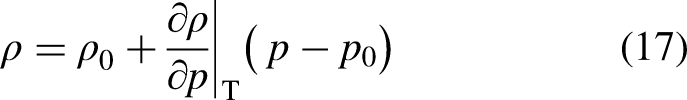$\rho$ to its old value ${\rho }_0$ and the changes in pressure. Due to this approach as shown in equation (17), we refer to the solver as weakly compressible.

$$\rho ={\rho }_0+{\frac{\mathrm{\partial }\rho }{\mathrm{\partial }p}|}_{\mathrm{T}}(p-p_0)$$

(17)

Liquid fuel combustion

Fuel droplets are introduced into the computational domain within the shear region to closely match the hybrid atomization process. The droplet diameters are defined by means of a Rosin Rammler size distribution according to equation (18) that defines the mass fraction 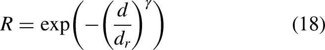$R$ above a given droplet diameter according to droplet size $d$ and a diameter dispersion parameter $\gamma$ . The drag force acting on the coupled droplet momentum transfer is described by a modified Schiller–Naumann drag model in order to limit the behavior in the inertial regime as seen in equation (19). The Ranz–Marshall correlation was adopted for the overall droplet heat transfer coefficient which relates the Nusselt number to Prandtl and Reynold numbers for flow past spherical particles according to equation (20). The mass transfer that defines the evaporation process is then calculated based on whether the evaporation falls above or below the droplet boiling temperature as formulated in equation (21). ³³ This depends on the particle dynamic diffusivity $\rho D$ , Sherwood number $Sh$ , molecular weights of the vapor and mixture in the continuous phase, $W_{\mathrm{C}}$ and $W_{\mathrm{G}}$ , as well as the molar fraction in the gaseous phase $X_v^V$ and equilibrium molar fraction at droplet surface $X_S^V$ . In the case that the droplet’s total vapor pressure $p_{\mathrm{v},\mathrm{tot}}$ is larger than its surrounding gas pressure $p_{\mathrm{amb}}$ the droplet is assumed to be under boiling conditions. The evaporation rate is then calculated using the ratio between the heat transfer to the droplet $Q_p$ and the latent heat of evaporation $Q_{\mathrm{evap}}$ .

$$R=\exp (-{\left(\frac{d}{d_r}\right)}^{\gamma })$$

(18)

$$C_D=max(\frac{24}{Re}(1+0.15R{e}^{0.687}),0.44)$$

(19)

$$\begin{array}{cc}& Nu=2+0.6R{e}^{0.5}P{r}^{0.3}\\ & 0\le Re<200\text{and}0\le Pr<250\end{array}$$

(20)

$$S_{c,l}=-S_{c,g}=\{\begin{array}{c}\pi d_p\rho DSh\frac{W_{\mathrm{C}}}{W_{\mathrm{G}}}\ln \left(\frac{1-X_S^V}{1-X_v^V}\right)\\ -\frac{Q_p}{Q_{\mathrm{evap}}}\text{ if boiling}\end{array}$$

(21)

Liquid fuel measurements

In order to characterize the liquid fuel atomization, experimental analysis was conducted to study the droplet size distribution downstream of the burner using phase Doppler anemometry (PDA). The burner operates under pressurized conditions and has poor optical accessibility in the atomization region, which prohibits the use of the PDA system on-site at UT. The experimental spray test facility at KIT aimed to make the measurements possible at a recreated setup with improved optical accessibility. This setup included a compressor, which supplied the system with air at atmospheric conditions, while water was fed by means of pressurized vessels. A hollow cone nozzle was used for the injection of water inside the airblast atomizer. The water was collected in a tank after being sprayed, while a vacuum pump was used to ensure that no droplet recirculation occurs in the surrounding air that might affect the data acquisition process. In a pre-filming airblast atomizer, the liquid accumulation acts as a buffer that decouples the film flow and the breakup process and diminishes the importance of liquid injection prior to pre-filming. ³⁴ It should be noted, however, that the smaller droplets are expected to be slightly underrepresented due to our atmospheric measurement setup.

The produced spray was characterized by a commercial PDA system, involving a receiver with three detectors at an off-axis angle of 30 $\circ$ . The laser used was a diode-pumped solid-state employing laser beams at wavelengths of 532 nm and 561 nm. The axial velocity component, as well as the diameter of the droplets, were measured by utilizing the 532 nm laser, while the 561 nm laser provided information on the radial velocity component. This configuration, taking into account the wavelength of the laser beams, the beam spacing, and their intersection angle, creates a measurement volume with a diameter of roughly 154  $\mu$ m and a length of roughly 2.7 mm, allowing measurement for droplet diameters up to approximately 300  $\mu$ m. The measurement technique was mounted on a three-axis translation system so that various positions in the spray region could be investigated as illustrated in Figure 4. A grid of measurement positions was identified and on each measured location, 50,000 droplet samples were acquired, containing information about the two velocity components as well as the diameter of each individual droplet.

Figure 4.

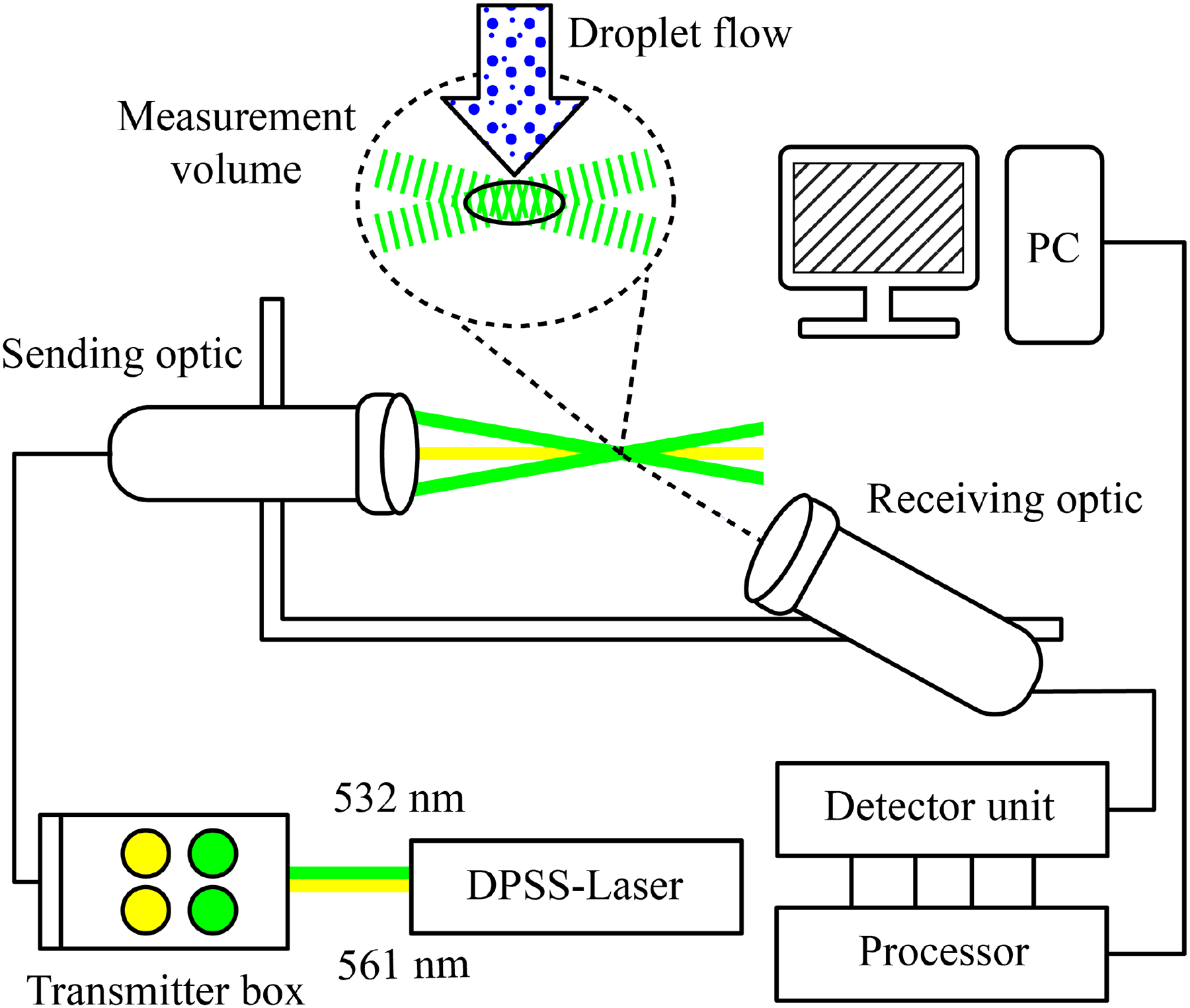
Phase Doppler anemometry (PDA) measurement configuration schematic.

The experimental measurement points are situated in a Cartesian grid downstream of the dump plane and cover a radial distance $r_{max}=60\mathrm{mm}$ and four equidistant axial locations ranging from $y/R=0.36$ to $y/R=1.24$ . The measured Sauter mean diameter (SMD, $D_{32}$ ) contour plot is presented on the right side in Figure 5. On the left, the measured droplet mean velocity vector field is overlaid on top of the mean filtered velocity contour plot. The experimental measurement grid is denoted by means of a Cartesian grid of markers. The measurement results show the high droplet velocity region occurring at around $r/r_{max}=0.4$ together with a significant reverse flow region closer to the centerline which builds up a relatively strong vortex breakdown region downstream of the swirl burner and provides an aerodynamic body for flame anchoring. The measured SMD values denote the presence of larger droplets farther from the centerline with the smaller droplets being able to follow the flow within the vortex core and into the flow reversal region.

Figure 5.

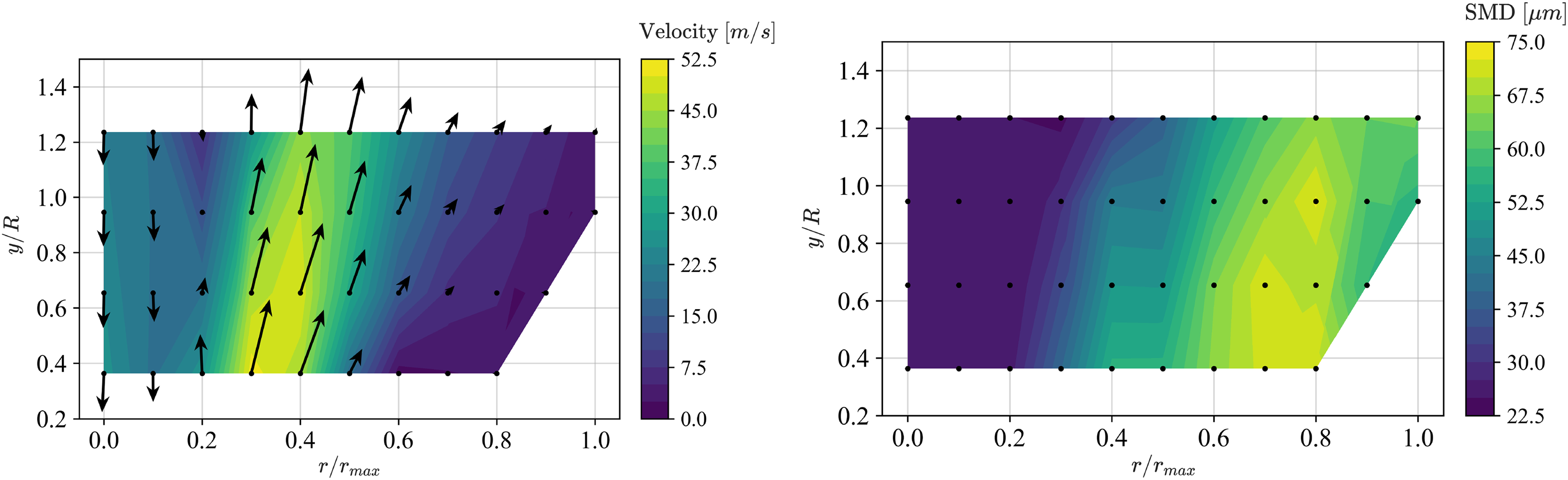
Experimental measurement results downstream of the burner plotted over normalized radial and axial distance from dump plane. Droplet velocity contour and vector plots (left) and droplet Sauter mean diameter (SMD) (right).

Based on the droplet density ${\rho }_d$ , diameter $d_r$ , and dynamic viscosity ${\mu }_g$ as reported in Table 2, the characteristic time of the droplets ${\tau }_0=6.74\times {10}^{-4}4\mathrm{s}$ is found to be smaller than the flow residence time through the burner $t_r\approx 3\times {10}^{-3}\mathrm{s}$ . The resulting Stokes number $Stk\approx 0.22$ indicates a small slip velocity between the liquid droplets and their immediate surrounding air. Here, we make use of this fact and take the experimentally measured droplet velocity to be very close to the air velocity. Nonetheless, this assumption contains errors and is only made for the purpose of establishing a comparison.

Table 2.

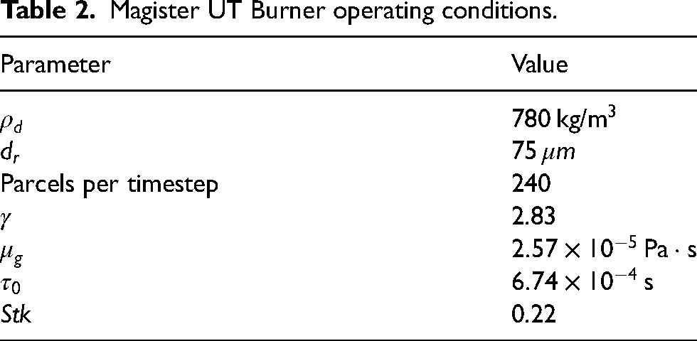
Magister UT Burner operating conditions.

Parameter	Value
${\rho }_d$	780 kg/m3
$d_r$	$75\mu m$
Parcels per timestep	240
$\gamma$	2.83
${\mu }_g$	$2.57\times {10}^{-5}\mathrm{Pa}\cdot \mathrm{s}$
${\tau }_0$	$6.74\times {10}^{-4}\mathrm{s}$
$Stk$	0.22

In order to compare the experimental measurements to simulated results, we consider two different numerical simulations to account for the discrepancy between the UT and KIT setups. The first and last axial locations are selected and the mean value of measured droplet axial velocity is compared to time-averaged simulated axial flow velocity as presented in Figure 6. The blue line shows the simulation results for an enlarged combustion chamber by a factor of two in all directions to relax the effect of chamber walls. The combustion chamber walls affect the shape of the vortex breakdown region and the expansion of the flow downstream of the burner and their absence contributes to differences between measured and simulated values shown. The black line retains the actual operating geometry of the burner. The error bars display one standard deviation for each measurement position. It should be mentioned that the standard error of the mean measurement is negligible due to the large sample sizes of around 50,000 measurements for each location. The simulation methodology appears to be adequate in capturing the correct flow pattern when geometry discrepancies are accounted for. It can be seen that the time-averaged DES results in the UT setup (black line) is able to reproduce the prominent reverse flow closest to the dump plane at $-$ 27.93 m/s compared to the measured mean value of $-$ 26.2 m/s with an error of 6.2%. This error is further reduced for the farther axial locations. The maximum axial velocity value appears to be simulated well within the measurement confidence interval. The location at which the maximum axial velocity occurs, however, is measured slightly closer to the centerline compared to UT DES results as well as having a relatively wide confidence margin.

Figure 6.

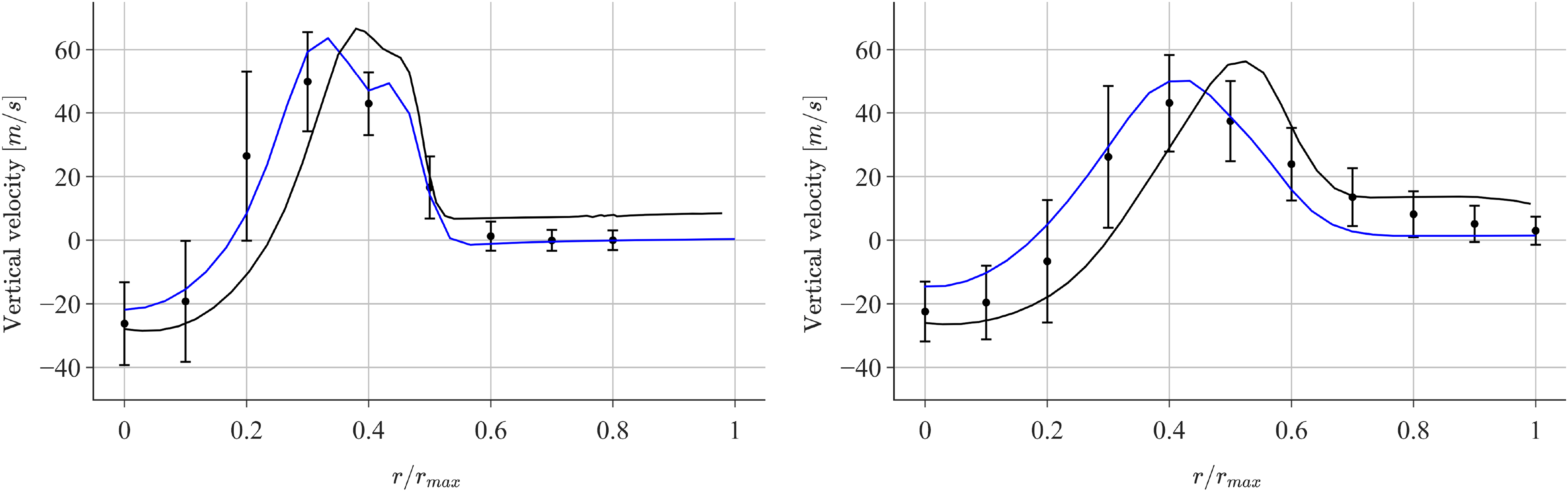
Comparison between axial velocity of time-averaged detached eddy simulation (DES) (burner combustion chamber geometry in black and enlarged chamber in blue) and experimental measurements (dots) at axial locations of $y/R=0.36$ (left) and $y/R=1.24$ (right). Error bars indicate standard deviation of measured values.

Inferring a suitable droplet size distribution based on downstream measurements is a challenging task. Similar airblast swirl burners have been investigated in the literature suggesting the suitability of the Rosin Rammler distribution function.^35–37 Considering the low Stokes number of the droplets, measurement locations that are situated within the high-speed flow near $r/r_{max}$ =0.4 were selected for defining the distribution function. The distribution as defined in equation (18) is based on the assumption that an exponential relationship exists between droplet diameters and the specified rosin diameter $d_r$ such that 63.2% of the droplet mass fraction fall below the rosin diameter which for the present experimental data, results in rosin diameter of $d_r=75\mu m$ . The dispersion parameter was found by means of a least squares minimization in order to find the optimal fit to the experimental data corresponding to $\gamma =2.83$ . The resulting distribution closely matches the observed droplet distribution with a slight over-representation for the largest droplets as shown in Figure 7.

Figure 7.

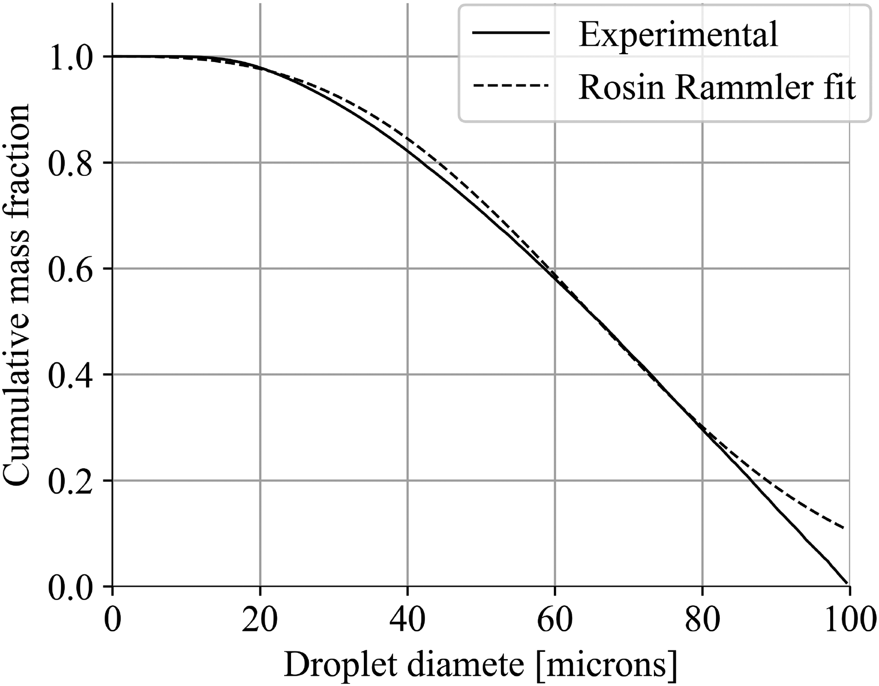
Cumulative mass fraction for measured droplets compared to the Rosin Rammler fitted curve.

POD formulation in PARAMOUNT

A generic time-variant parametric dynamical system is represented by means of a separation of variables method to distinguish between the spatial (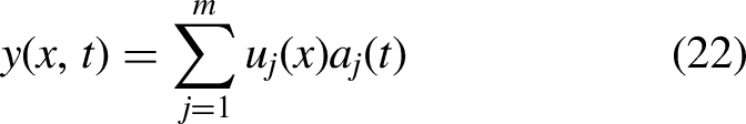 $x$ ) and temporal ( $t$ ) dimensions.

$$y(x,t)=\sum _{j=1}^m{u}_j(x)a_j(t)$$

(22)

where $m$ represents the number of modes used to describe the time-varying dynamical system that exists in Hilbert space $L^2$ . POD provides a basis to find such decomposition with the condition of optimality, that is, finding the most efficient way of capturing the dominant components of an infinite dimensional continuous dynamic system with only a finite number of modes. ³⁸ We can further elaborate this formulation by means of an assembly matrix $Y$ that contains a finite ensemble of discrete samples with $m$ temporal snapshots and $n$ spatial degrees of freedom.

$$Y=\left[\begin{array}{cccc}y(x_1,t_1)& y(x_1,t_2)& ...& y(x_1,t_m)\\ y(x_2,t_1)& y(x_2,t_2)& ...& y(x_2,t_m)\\ ⋮& ⋮& \ddots & ⋮\\ y(x_n,t_1)& y(x_n,t_2)& ...& y(x_n,t_m)\end{array}\right]$$

(23)

POD is thus formulated as the singular value decomposition of matrix $Y$ , which results in the following relationship between the columnar matrix of eigenvectors $U$ , the singular values diagonal matrix $\mathrm{\Sigma }$ , and the row coefficient matrix $V*$ .

$$Y=U\mathrm{\Sigma }V*\approx U_r{\mathrm{\Sigma }}_r{V}_r*$$

(24)

With left singular matrix $U$ containing the spatially orthonormal basis functions and right singular matrix $V*$ containing the conjugate transpose matrix of time-dependent orthonormal amplitude coefficients. POD algorithm produces the diagonal matrix $\mathrm{\Sigma }=\mathrm{diag}[{\sigma }_1,{\sigma }_2,\dots ,{\sigma }_r]$ containing the eigenvalues of the decomposition in descending order based on their energy contributions.^39,40 The relationship between total $L^2$ -norm mode energy $\sum _{j=1}^m{\sigma }_j^2$ and the kinetic energy present in the flow is valid only if the temporal and spatial discretization are cartesian, however, in a real flow application, this relationship can still provide insight into identifying major energy-carrying flow structures. ⁴¹ In this way, the truncation value $r$ is arbitrarily chosen to downsize the full SVD matrix and focus on the top most energetic modes with the energy contribution of the i^th mode defined in equation (25).

$$E_i={\sigma }_i^2/\sum _{j=1}^m{\sigma }_j^2$$

(25)

The underlying SVD decomposition as presented in equation (24) is typically computed using the fast, efficient, and well-tested software package LAPACK used in many available computational tools. It uses a divide-and-conquer algorithm to compute the three singular value matrices. ⁴² The underlying data in fluid flow analysis and CFD is typically very rich in space with number $n\gg m$ resulting in a “tall and skinny” $Y$ matrix, which contributes to a more efficient computation of SVD, yet the computed data in LES or Domain Name System analysis is still in the order of terabytes. Working with such large datasets can pose some challenges in computing the SVD. First, most time-dependent results are stored in a time-indexed database and the variable of interest needs to be gathered from each stored dataset and collected into a final assembly matrix $Y$ . Second, the final size of the assembly matrix $Y$ can be too large for a successful calculation of SVD due to limitations in available memory. Finally, the analysis results could be prohibitively too large for post-processing in a two-dimensional (2D) or 3D framework and the relationship between the multitude of modes and their associated coefficients could be difficult to identify.

In order to address these challenges, we have developed the open-source software package PARAMOUNT. It utilizes Dask, which is a flexible library for parallel computing in Python and allows for dynamic task scheduling for optimizing computational workloads as well as handling large datasets.^43,44 Furthermore, it uses Apache Parquet file format, which is an efficient, structured, and column-oriented binary format capable of file size reduction and efficient reading of the desired stored values without the need to load the entire file into memory. ⁴⁵

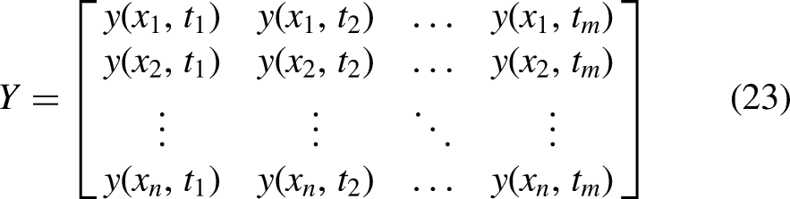
More concretely, to address the above-mentioned challenges, PARAMOUNT has been developed with the capability of assembling the data matrix $Y$ for a list of variables of interest. This is done by collecting each variable from the time-indexed database into its corresponding Parquet file and is performed in parallel to maximize the use of available computational resources. Second, the SVD is computed using Dask which allows for processing large data assembly matrices which cannot be simply loaded in memory in their entirety by dividing the stored variables into smaller chunks and computing the final $U$ , $\mathrm{\Sigma }$ and $V$ matrices in parallel each of which is stored in a corresponding Parquet file for further analysis. Finally, PARAMOUNT is able to visualize the results of modal analysis in terms of 2D and 3D mode shapes, mode energy contents, and spectral analysis of mode coefficients as well as self-correlation and cross-correlation maps for results of one or more decomposition analyses.

For 2D visualizations, a diverging color map is employed to highlight the flow structures. Additionally, a $k\text{-d}$ tree algorithm is employed to compute a nearest neighbor distance map for the provided data points. This map is used to mask out the regions that fall outside the computational domain but within the bounding box of POD analysis. For 3D visualizations, two isosurfaces are identified countering the mean value of the mode shapes in order to show the flow pattern structures in 3D with options to fine-tune their positions and opacity.

In order to establish correlations between modes, a correlation index is formulated based on the Pearson product–moment correlation as shown in equation (26). This is done due to this correlation being invariant under separate changes in location and scale between two variables. ⁴⁶ The implemented correlation algorithm accounts for possible time lag present between the variables which in the context of a fluid dynamics system can be of a convective nature or simply due to non-synchronized data acquisition.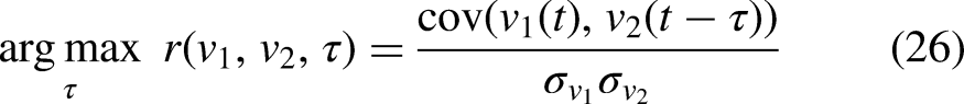

$$\underset{\tau }{\arg \max }r(v_1,v_2,\tau )=\frac{\mathrm{cov}(v_1(t),v_2(t-\tau ))}{{\sigma }_{v_1}{\sigma }_{v_2}}$$

(26)

With $v_1(t)$ and $v_2(t)$ being two sampled variables in time, $\sigma$ the standard deviation for each variable, and $\tau$ the time lag for which the two signals exhibit maximum linear correlation. Pairwise computation of this correlation index allows us to create correlation heatmaps with easy comparison between a multitude of modes across all the variables of interest which can be performed as self-correlation between modes for a given POD analysis or as cross-correlation between modes of two separate POD analysis. In the latter case, the correlation heatmap can identify the effects of modifications to the underlying dataset, for example, effects of acoustic forcing or a change in ambient temperature can be investigated by means of cross-correlation between modes of the two POD analysis results. This can identify the way in which modes react to the specific changes and how they dynamically gained or lost correlation with other modes in the analysis.

The spectral content of mode coefficients is further analyzed by applying Welch’s overlapped segment averaging periodogram with a Hann window to the detrended coefficient values. The resulting PSD figures represent the dominant frequencies at which each mode is mainly active.

Results and discussion

Detached eddy simulation

Figure 8 shows the snapshot contour plots for temperature, velocity, and pressure. The velocity contour plot shows the region of high shear between the two sets of air entry ducts present in the swirl burner. The V-shaped regions of high velocity in the 2D cross-section plane form the aerodynamic body that defines the central recirculation zones (CRZs). The flow reversal reaches all the way back inside the burner where the liquid fuel injector is located. The temperature contour plot shows the region at which liquid fuel is injected with the combustion in the gaseous phase producing the pockets of high temperature downstream of the burner. The heat release continues as the droplets evaporate and combust farther away from their injection location. The regions of high temperature are also observed to be convected back inside the burner within the CRZ. The pressure contour plot shows a region of lower pressure in the core of the swirler which is formed as the flow leaves the swirler and enters the combustion chamber. This causes a flow reversal in the vortex breakdown region. Multiple regions of lower pressure shedding can be identified that originate at the base of the swirler and convect downstream in a specific pattern. The domain of flow reversal is outlined using a zero axial velocity contour overlaid on the pressure contour.

Figure 8.

Top row: two-dimensional (2D) contours of time-averaged values for temperature (left), velocity (center), and pressure (right). Bottom row: instantaneous values overlaid with zero axial velocity for pressure contour.

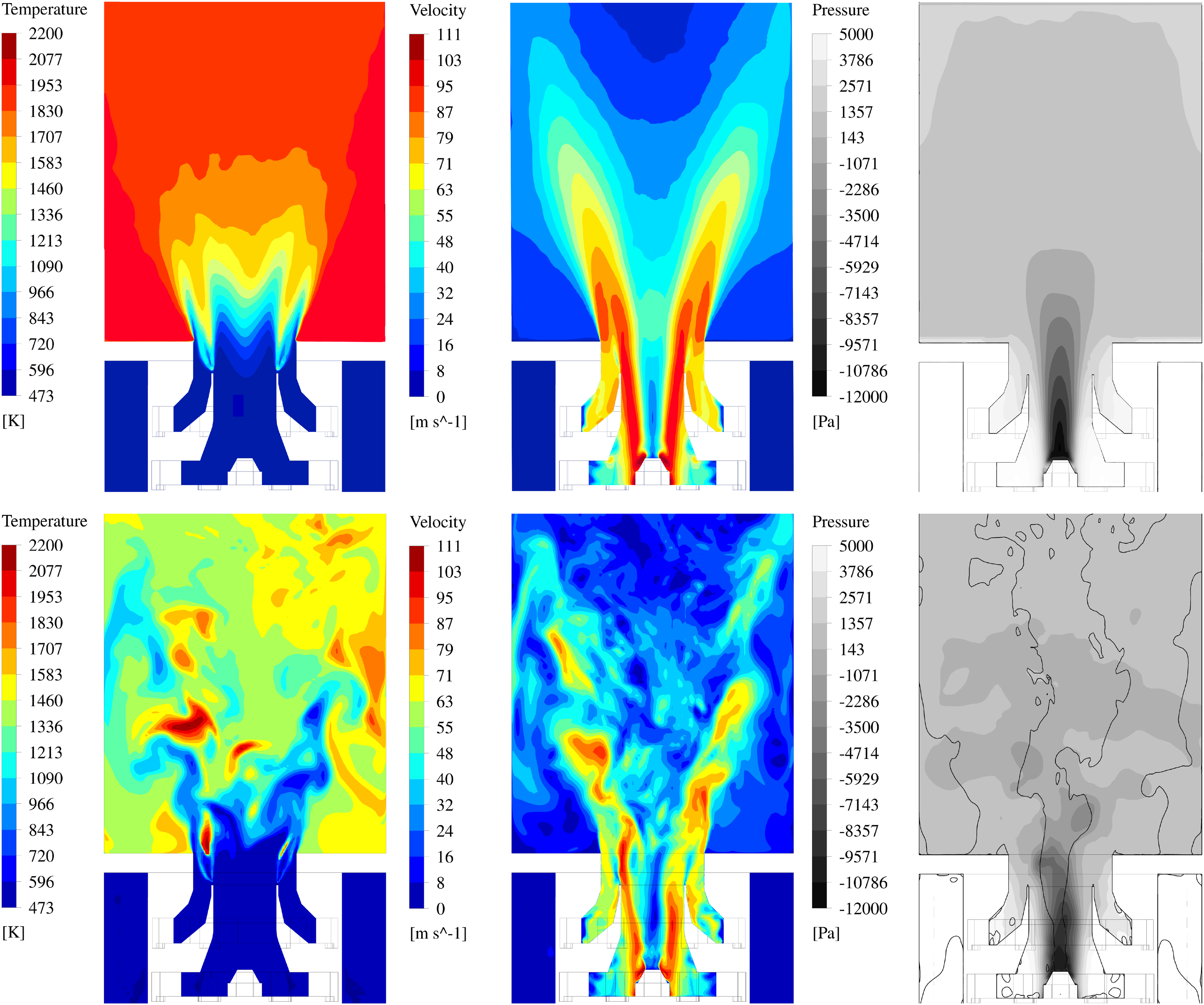
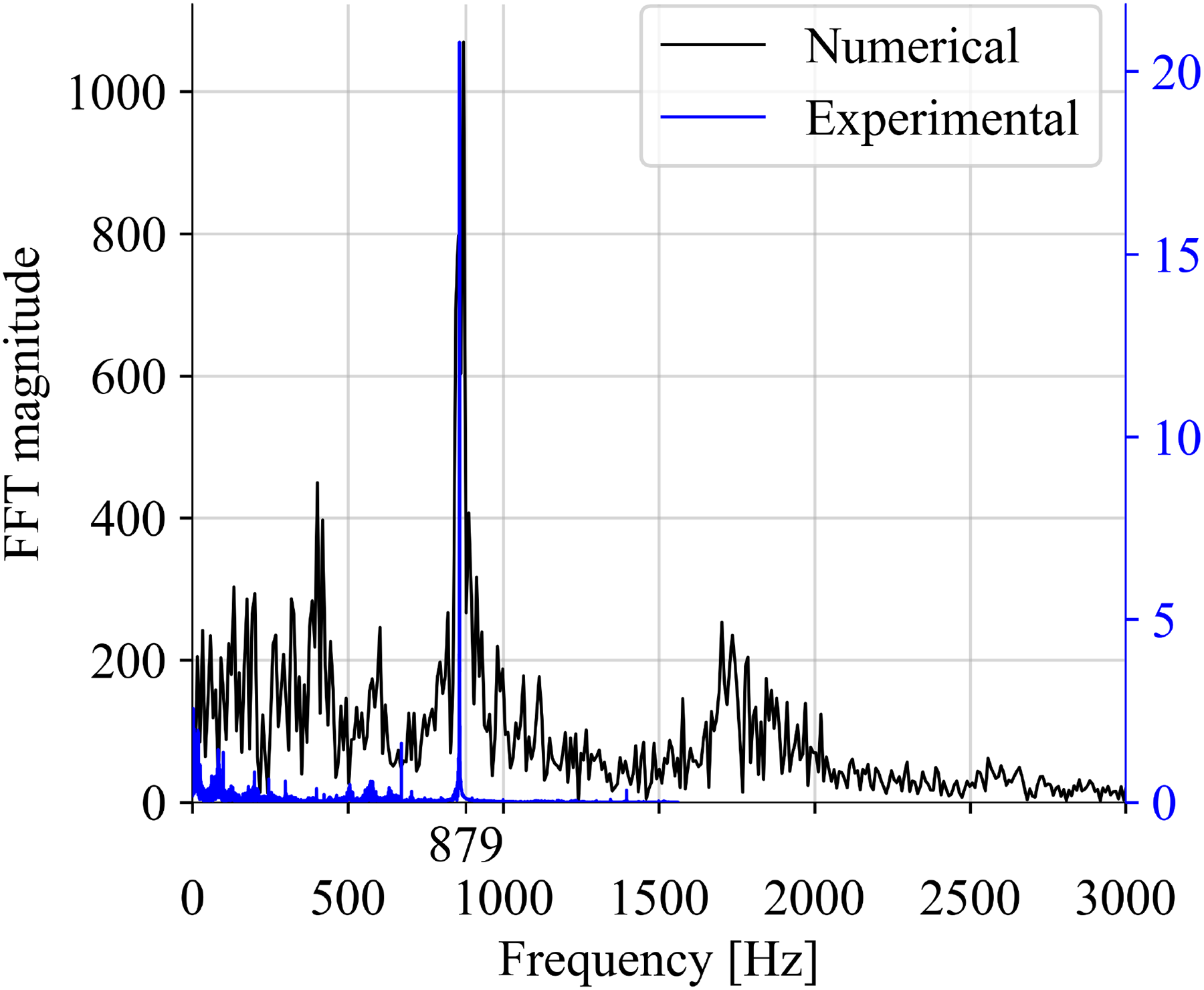
The flow exhibits a high degree of periodicity and certain flow structures can be visually identified. As an example, extracted pressure time series from a point located near the negative gauge pressure region exhibits the spectral content shown in Figure 9 with a distinctive peak at around 879 Hz, which we identify as the presence of a PVC at the base of the swirler. This method of numerical analysis appears to be highly sensitive to the data extraction point and also sensitive to transient phenomena in order to ensure the identification of such flow structures and their associated dominant frequency a careful analysis of flow evolution is required together with multiple points of data extraction in the near swirler region. It is noteworthy that the frequency of the PVC in similar studied burners varies greatly between 400 and 2000 Hz and depends greatly on the inlet velocity and the velocity gradients in the inner swirling region.^21,19,20,22 Figure 10 depicts the instantaneous Lambda-2 criterion visualization of the vortex core region colored by axial velocity. The PVC can be identified as the dominant swirling vortical structure that originates at the base of the burner and spirals downstream in a helical fashion.

Figure 9.

Fast Fourier transform of simulated extracted pressure time series located inside the swirler compared to cold flow experimental pressure transducer measurements located in the combustion chamber.

Figure 10.

Lambda-2 criterion visualization of the precessing vortex core (PVC) and the vortex breakdown region colored by axial velocity.

Figure 9 also includes preliminary cold flow experimental measurements from our pressurized test facility at the University of Twente taken from a pressure transducer located on the combustion liner further downstream in the combustion chamber. The cold flow experimental data appears to be in perfect agreement with DES results in terms of significant spectral content at the PVC frequency. It should be noted that this peak is much less prevalent in preliminary combustion experiments as the turbulent reacting flow caused spectral change in pressure at the measurement location.

Proper orthogonal decomposition

The variables of interest in this study include pressure $p$ , temperature $T$ , mass fraction of OH radicals, axial velocity $V_v$ , and two rotational velocity components in the dump plane $V_u$ and $V_w$ . For the 2D analysis, these variables are extracted from a cross-section plane traversing the computational domain. The 2D plane includes the upstream casing, the burner, and the combustion chamber and partially includes the angled primary and secondary entry ducts. For the 3D analysis, the variables are extracted using a point cloud scattered throughout the computational domain such that the total number of recorded points remains the same between the two at around 100,000. The $Y$ matrix is assembled for each variable and stored in their respective parquet database. The number of flow snapshots considered in the analysis was chosen as $n=3000$ corresponding to about 105 periods of precessions for the PVC. This decision was made with the consideration of achieving a suitable degree of convergence for the flow structures close to the expected PVC frequency while maintaining an acceptable number of periods for flow features at lower frequencies. Next, the SVD is computed for each variable and the resulting decomposition matrices are stored using PARAMOUNT. The mode shapes are visualized by means of a linear interpolation of the $U$ matrix over a uniform and fine Cartesian grid for both 2D and 3D cases. A diverging color map is employed to emphasize regions of contrasting value such as the near flame region where the presence of strong velocity and pressure gradients are to be expected. This allows for qualitative comparison and interpretation of mode shapes and their physical meaning.

Figure 11 shows the first five POD analysis mode shapes for the variables of interest. 3D mode shapes are presented where they could convey the mode shape better, otherwise, the 2D mode shapes are presented. The first mode is indexed “0” to reflect the fact that it is simply the time-averaged DES data and thus different from other modes in nature.

Figure 11.

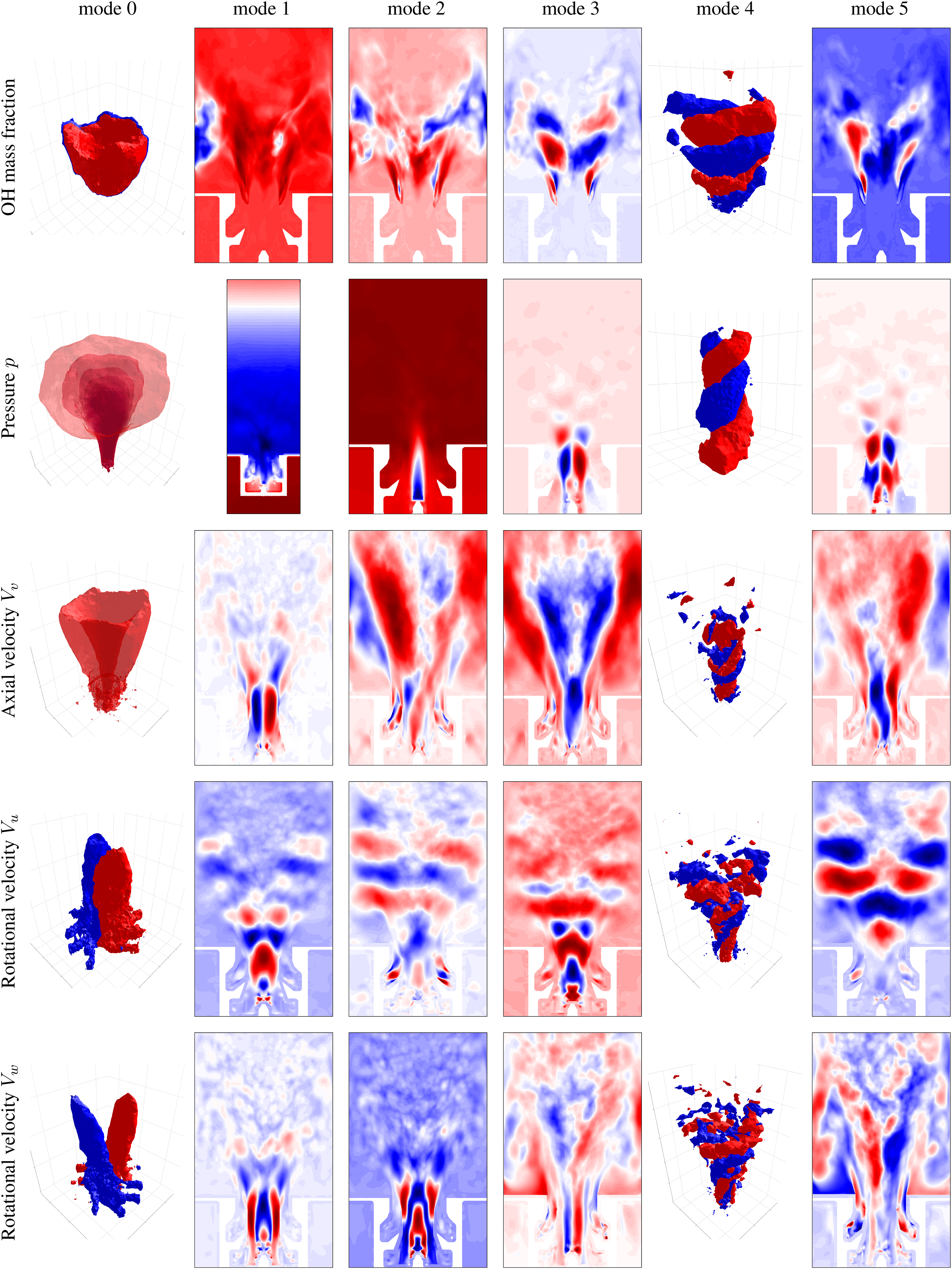
First five POD mode shapes for the mass fraction of OH radicals in the first row, pressure $p$ in the second row, Three velocity components of axial velocity $V_v$ and the two components of rotational velocity in the dump plane, $V_u$ and $V_w$ in the bottom rows, respectively. Some modes are presented in 3D to better convey their properties. POD: proper orthogonal decomposition; 3D: three-dimensional.

The heat release indicator in this analysis is the OH mass fraction as presented in the top row. The release of the liquid fuel droplets is randomized in time and their time-averaged 3D mode shows a hollow cone 3D structure for mode “0” that reflects where the flame is sitting in the simulation. Randomized entry of droplets can be seen to have an effect on the symmetricity of this mode, causing the downstream edges of the isosurface to appear at different axial distances. The first POD mode for OH mass fractions does highlight the two wings of the flame represented in 2D, but also demonstrates the wall interaction that the flame has had for the duration of the simulation. Modes 3 to 5 represent the coherent flow structures as it relates to the swirl present in the flow with mode 4 showing the spiral nature of the two isosurfaces in 3D. Other possible choices for the heat release rate indicator are CH radicals, RPV, or temperature. These mode shapes appeared to be highly similar to those of the OH mass fractions and therefore omitted for brevity.

Pressure mode shapes are of high interest because the flow solver is weakly compressible in nature and thus pressure plays an important role in shaping the velocity field. The first pressure mode indexed “0” represents the time-averaged DES results with a low-pressure core sitting at the base of the burner just above the liquid injector. Multiple isosurfaces are drawn to show the progressive opening of the flow outside the burner. The degree of the opening of this mode is shaped by the primary and secondary air entry ducts and the degree of induced swirl in each of them. The first POD mode is best shown as a zoomed-out view of the computation domain since it relates to the axial pressure gradient presented by various flat isobaric planes which are formed more prominently just outside the burner and continue in the axial direction toward the flow outlet. The second and third pressure modes represent a monopole and a dipole situated at the base of the burner. The monopole appears to be driving the axial spectral content and the dipole appears to be the main generator for the swirl present in the burner. As an example, the fourth mode is shown in 3D to highlight how the 3D helical structure of PVC contributes to the swirl present in the flow.

The three velocity components are presented in the bottom rows of Figure 11. The time-averaged vertical velocity highlights the region of high velocity created both by the swirler geometry and bolstered by the extreme expansions caused by combustion. This mode is shown with a lower opacity scale to demonstrate the hollow cone nature of this structure. CRZ is enveloped by this mode and creates the main dynamic body that stabilizes the flame. The time-averaged modes for the other two velocity components are similar in shape and appear to be rotated by $90\circ$ along the axial direction with respect to each other. This is expected as the rotating flow causes a diverging flow in radial directions and is visualized by the two counter-positioned isosurfaces showing half of air entry ducts acting together to induce swirl. Other velocity modes show strongly coherent structures that represent diverging mode values that alternate in space and demonstrate the degree of high periodicity exhibited by the swirl burner.

Mode shapes are able to convey how various flow features are shaped in space and their corresponding mode coefficients show how they have behaved in time. The nature of POD mode coefficients lacks a certain degree of time dynamics that could show how these modes could further evolve in time similar to other spectral methods such as dynamic mode decomposition, yet a spectral approach to mode coefficient analysis reveals the main frequencies associated with each coefficient. Here, we have used Welch’s overlapped segment averaging periodogram to identify the main spectral content for each mode. The notable peaks in the PSD chart are highlighted for ease of reference. As an example, Figure 12 shows the PSD analysis results for a number of axial velocity modes with significant spectral content at around 879 Hz which is associated with the PVC. It is important to note that this is not sensitive to any specific point extraction of the data and comes as the result of data-driven spectral POD analysis and is thus suited to flows for which a prior intuition or knowledge about their dynamics does not exist.

Figure 12.

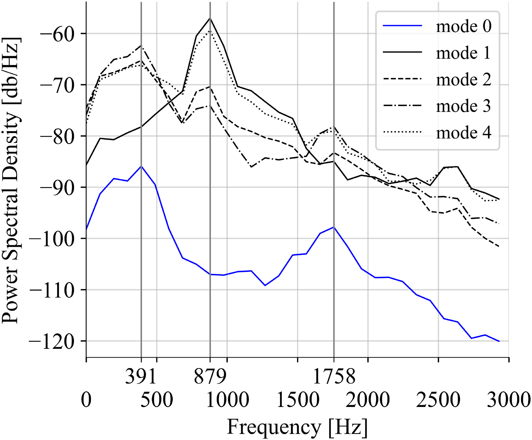
PSD for the first five POD mode coefficients of axial velocity. PSD: power spectral density; POD: proper orthogonal decomposition.

The spectral content is analyzed for all considered mode coefficients and certain frequencies are observed to be predominantly present for a variety of modes. For example, 98 Hz and 195 Hz are identified in the first and second modes for pressure and OH mass fraction variables in the lower frequency range. At higher frequencies, 391 Hz and 879 Hz are identified in the third and fourth velocity modes as presented in Figure 12. These examples appear to be identifying certain harmonics with almost doubling of values for each frequency range and associated with different flow structures, for example, 195 Hz representing a dominant axial acoustic mode present in the domain and 879 Hz representing the dominant swirling motion present in the PVC.

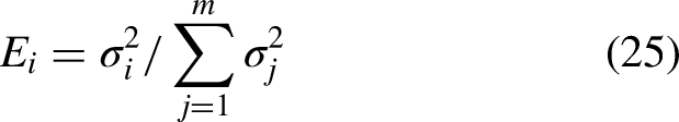
Another important aspect of the POD analysis is the eigenvalues of the singular decomposition as formulated in equation (25). The POD modes are ranked according to their total Frobenius norm $L^2$ -norm mode energy, which in this case, translates to total carrying kinetic energy. ⁴⁷ Figure 13 summarizes the cumulative energy contribution per mode for all considered variables.

Figure 13.

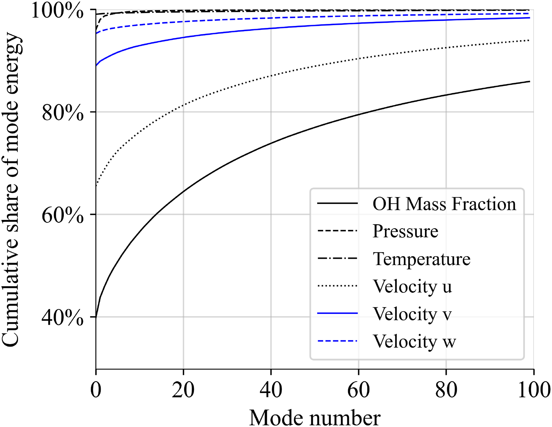
Mode energy content for all considered variables.

When the very first mode already contains the majority of energy content, for example, temperature and velocity component, it can be concluded that the first mode and its associated frequency is significant in the behavior of the dynamic system, and a high level of periodicity is observed in those variables. This is in contrast to a variable such as OH mass fractions, which are chosen as a representation of where the flame front exists. The dominance of the first mode in terms of its energy content is much lower at around 40%, which demonstrates a lower degree of periodicity. This can be explained by the random nature of the release of liquid droplets in time and space which also makes for lower coherence in OH mass fraction mode shapes.

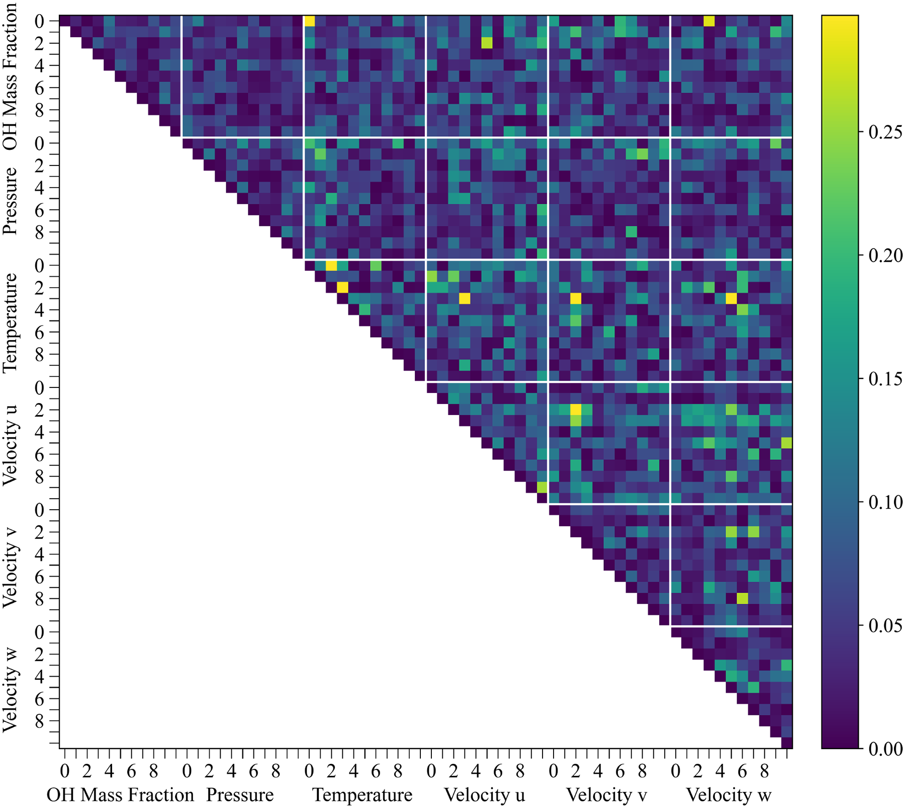
With the multitude of mode shapes and coefficients for each considered variable, it can be challenging to establish how the modes are related to each other which is largely left to pairwise inspection and subject to interpretation. We introduce a methodology to study mode coefficients and objectively establish their relationship with each other and their evolution when subject to external modifications and perturbations. To this end, heatmaps are used to identify a linear correlation between pairs of mode coefficients once using a standard Pearson’s correlation formulation and once as described in the adjusted correlation methodology introduced in equation (26). Figure 14 shows the results of this analysis. The lower triangular matrix represents Pearson’s correlation index for each mode pair with the diagonal self-correlation showing the maximum value of 1. The upper triangle shows the adjusted correlation index accounting for the possible time lag present between the corresponding mode pair. It can be observed that accounting for the time lag between coefficients of different modes (upper triangle), can identify correlated mode pairs more clearly, for example, non-axial components of velocity which are associated with the swirl present in the flow appear to be highly correlated with the third and fifth mode of pressure as well as significantly uncorrelated to the temperature modes. Other weak correlations can be noted such as the third mode of OH mass fractions with a dominant associated frequency of 879 Hz associated with the PVC. It should be noted that the third OH mass fraction mode is the only mode for that variable that exhibits that specific spectral content. Some correlations can only be observed after time lag adjustments such as the correlations for the first three pressure modes with other variables.

Figure 14.

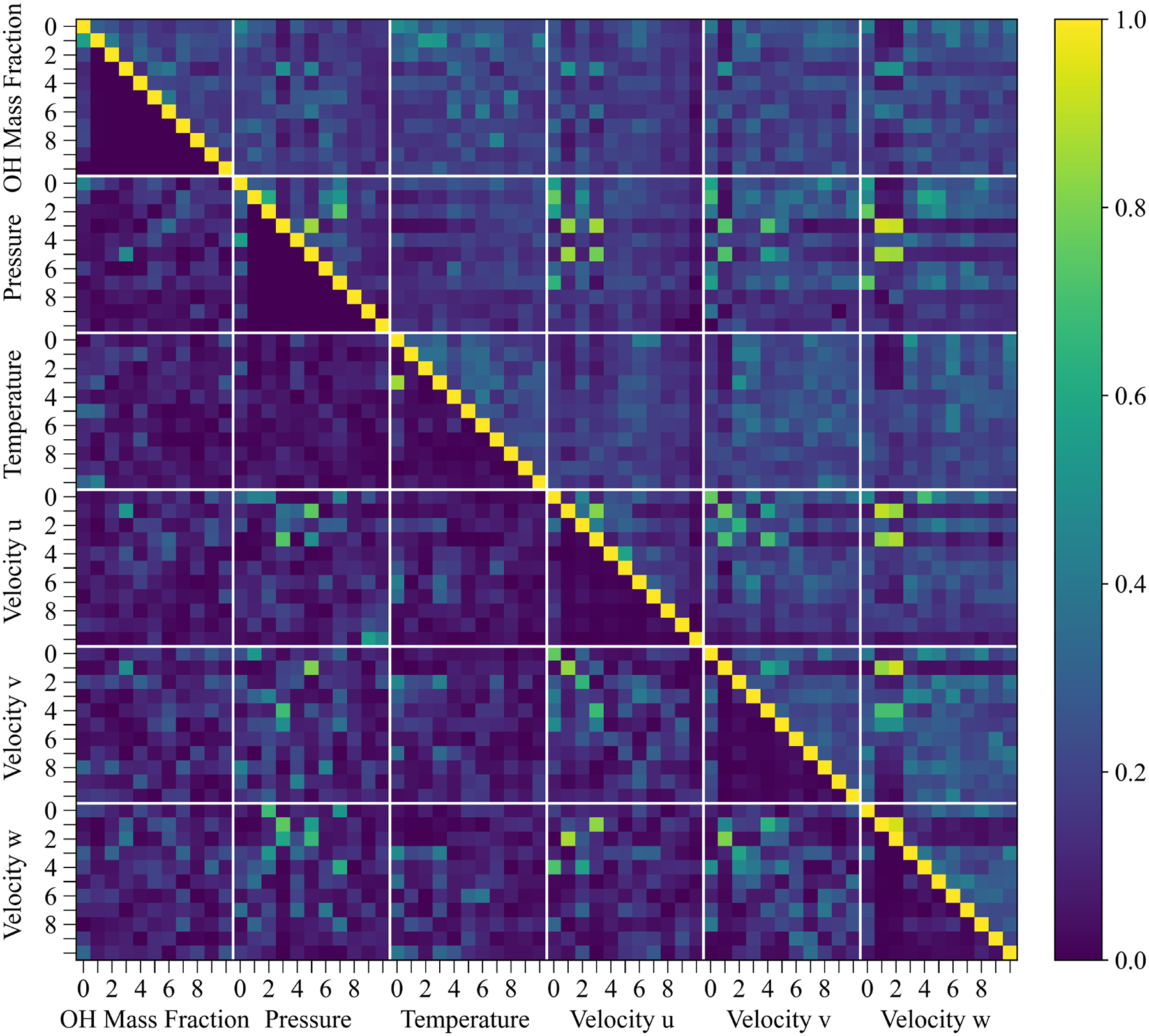
Correlation heatmap between first 10 POD mode coefficients of the unforced DES results. Pearson’s index in the lower triangle and adjusted value in the upper triangle. POD: proper orthogonal decomposition; DES: detached eddy simulation.

Effects of external forcing

In order to study the evolution of POD modes subject to external perturbations of the dynamical system, we subjected the air inlet mass flow rate to acoustic forcing in a separate DES simulation. The forcing is implemented as an inlet velocity modulation ⁴⁸ with the following formulation:

$$\dot{m}(t)={\dot{m}}_0(1+0.15\sin (2\pi ft))$$

(27)

With ${\dot{m}}_0$ representing the mean inlet air mass flow rate with subcritical forcing ⁶ modulation at 15% with frequency $f$ selected to be close to the PVC frequency at 800 Hz. The simulation results are obtained and analyzed in the exact same manner as in the unforced case with the majority of resulting POD mode shapes being very similar to those presented earlier and thus omitted in favor of brevity. Here, the effect of acoustic forcing is visualized from a POD analysis perspective using a correlation heatmap. In order to see the effects of forcing on the various modes between the two simulations, the difference in lag-adjusted pairwise correlation values is plotted in a new heatmap as presented in Figure 15.

Figure 15.

Heatmap of change in pairwise correlations between the first 10 POD modes of unforced DES simulation (vertical axis) and the forced DES simulation (horizontal axis). POD: proper orthogonal decomposition; DES: detached eddy simulation.

This heatmap can be interpreted as the correlation gained or lost for each mode coefficient pair due to acoustic forcing. Notice the amount of correlation index changed in absolute terms is around 0.3 in the upper bound. The most prominent changes are observed for mode coefficients of temperature, for example, the third temperature mode has gained significant correlation with the three velocity components. This is also observed for OH mass fraction modes which had poor correlation with other modes prior to forcing. This hints at the forcing having established a correlation between the heat release phenomena and the forced velocity domain and could be explained by enhanced entrainment of liquid droplets and more synchronicity between the heat release patterns and the velocity field.

The same methodology was applied to the volume-integrated variables such as the reaction progress variable, OH mass fraction, and mixture fraction. The correlation between volume-integrated OH mass fraction and every POD coefficient for all considered variables is calculated once for the non-forced simulation and once for the simulation subject to forcing. The change in correlation between the two scenarios is presented in Figure 16. This approach easily identifies some distinct modes that reacted the most to the external forcing, for example, second mode of the axial velocity $V_v$ and the third mode of rotational velocity $V_w$ appear to have, respectively, gained and lost the most in terms of their correlation to the volume-integrated OH mass fraction.

Figure 16.

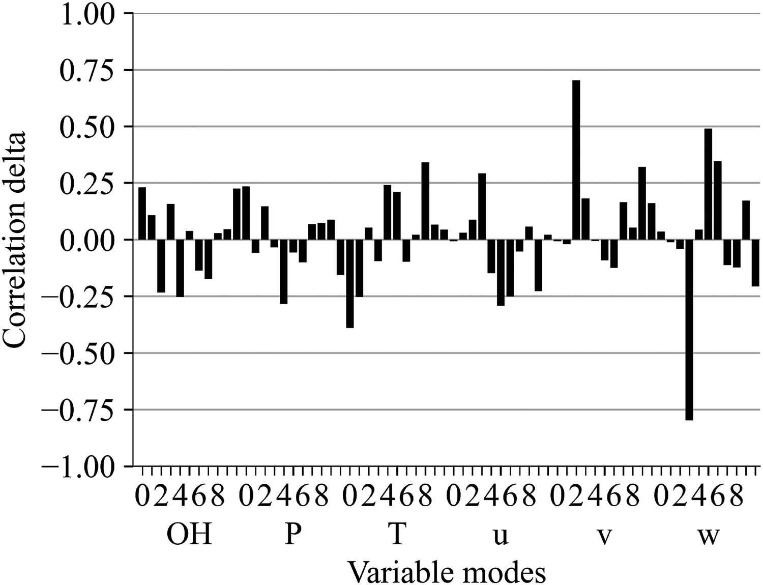
Change in the correlation of mode coefficients to volume-integrated OH mass fractions as a result of forcing.

The absolute change in this correlation delta ranks the order in which modes have reacted to the external forcing. 3D mode shapes for these two modes of interest are depicted in Figure 17. It can be observed that as a result of acoustic forcing, the central coherent structure for the second mode of axial velocity $V_v$ is more prominently located at the center of the swirler. The third mode of rotational velocity $V_w$ appears to have formed a more coherent structure with alternating patterns.

Figure 17.

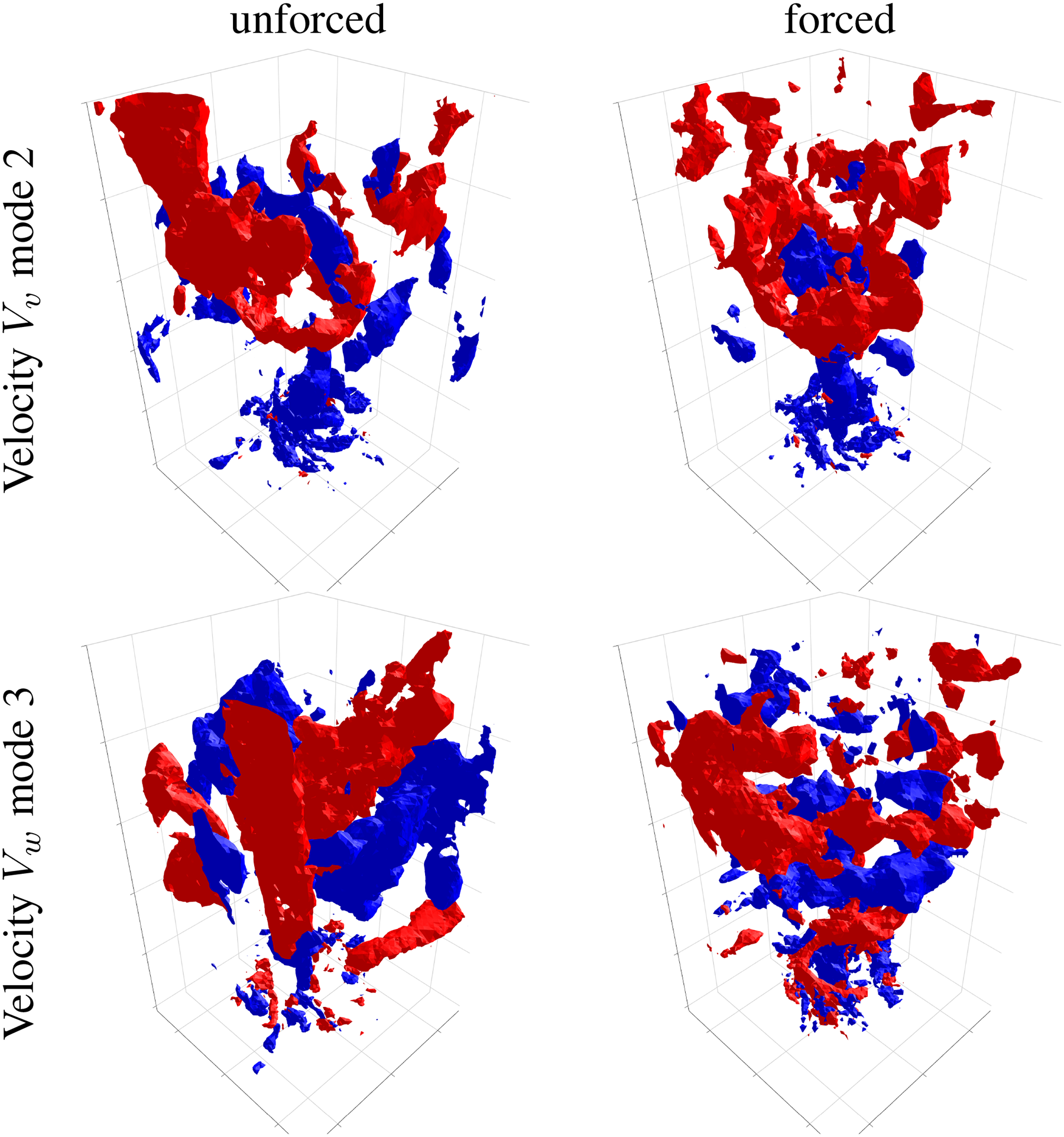
Change in mode shape as a result of forcing for the second mode of axial velocity $V_v$ and third mode of rotational velocity $V_w$ .

Conclusions

The study of aero engine representative burners is of great interest considering their environmental impact and their heightened sensitivity to thermoacoustic instability in lean conditions. LES remains an effective tool in the analysis of swirl stabilized burners resulting in large datasets that are suited to unsupervised modal analysis such as POD. The prohibitive computational requirements of both LES and POD make it challenging to consider non-premixed combustion regimes and investigate POD results not only across multiple flow variables, but also across various operating conditions. To that end, the in-house designed Magister UT burner was studied.

Non-premixed combustion is simulated at elevated pressure under two different inlet boundary conditions in a DES framework that shows to be in agreement with experimental observations and greatly reduces the computational requirements compared to a detailed LES approach. Combustion simulation results were analyzed using our modal analysis software package PARAMOUNT. This analysis addresses some fundamental difficulties associated with POD analysis by reducing computational requirements, providing cross-modal correlation analysis, and comparison of the results under different inlet operating conditions. The proposed correlation methodology was able to identify the specific ways in which the flow structures change subject to external forcing. As an example, specific velocity modes were observed to have gained coherence as a result of forcing, or in other words, the forcing manifests itself in terms of reshaping certain modes as identified by the correlation methodology.

The proposed acoustic characterization methodology appears effective in identifying the frequencies to which the burner might be most sensitive even while employing weakly compressible flow solvers. Additionally, this approach is effective in identifying influential modes that are otherwise insignificant in the context of a new operating condition. This information could be used to create improved reduced order models of the flow and provide insight into the pathways through which the external forcing manifests itself in the combustion process.