Incompressible versus compressible large eddy simulation for the identification of premixed flame dynamics

Abstract

The present work compares the respective advantages and disadvantages of compressible and incompressible computational fluid dynamics (CFD) formulations when used for the estimation of the acoustic flame response. The flame transfer function of a turbulent premixed swirl-stabilized burner is determined by applying system identification (SI) to time series data extracted from large eddy simulation (LES). By analyzing the quality of the results, the present study shows that incompressible simulations exhibit several advantages over their compressible counterpart with equal prediction of the flame dynamics. On the one hand, the forcing signals can be designed in such a way that desired statistical properties can be enhanced, while maintaining optimal values in the amplitude. On the other hand, computational costs are reduced and the implementation is fundamentally simpler due to the absence of acoustic wave propagation and corresponding resonances in the flame response or even self-excited acoustic oscillations. Such an increase in efficiency makes the incompressible CFD/SI modeling approach very appealing for the study of a wide variety of systems that rely on premixed combustion. In conclusion, the present study reveals that both methodologies predict the same flame dynamics, which confirms that incompressible simulation can be used for thermoacoustic analyses of acoustically compact velocity-sensitive flames.

Introduction

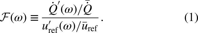
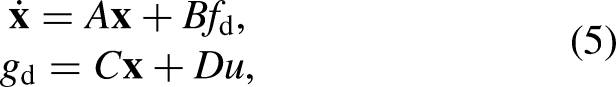
Investigating thermoacoustic combustion instability is crucial for the development of reliable, low-emission gas turbine engines. In these systems, combustion technology moves towards lean operating conditions in order to satisfy emission regulations on pollutants. Identification of a flame transfer function (FTF) is a key ingredient in the thermoacoustic stability analysis ¹ , as it is a necessary input for acoustic network models ² . The acoustic response of turbulent premixed burners can be described by a single-input-single-output ³ black box model, with velocity perturbations at a reference position as input and global heat release rate response as output. Given that perfectly premixed flames or configurations with an acoustically stiff fuel injector located very close to the burner outlet ⁴ are studied, the flame response is defined as

$$\mathcal{F}(\omega )\equiv \frac{{\dot{Q}}^{\mathrm{\prime }}\left(\omega \right)/\overline{\dot{Q}}}{u_{\mathrm{ref}}^{\mathrm{\prime }}\left(\omega \right)/{\overline{u}}_{\mathrm{ref}}}.$$

(1)

The established way in thermoacoustic studies to identify such a flame response is to use either experiment^5–8 or compressible large eddy simulation (LES)^9–12, where the flame is acoustically forced with a harmonic or broadband signal from an upstream or downstream position. Simultaneously, the velocity perturbations at the reference position and the global heat release signal are monitored. Such a procedure may be seen as “natural” and, accordingly, widespread in the thermoacoustic community. For example the works of Kaufmann et al. ¹³ , Giauque et al. ¹ , and Han and Morgans ¹⁴ mention:

The following requirements must be matched by the LES tool to obtain reliable information for flame transfer functions in gas turbines: 1) The full three dimensional compressible Navier Stokes equations must be solved on unstructured meshes for complex geometries. Kaufmann et al. (2002) ¹³

To determine the transfer function of a burner, the usual procedure is to introduce an acoustic wave into the burner (usually through the inlet) and measure the perturbation of heat release. Giauque et al. (2005) ¹

The need to include acoustic waves when considering the flame response means that compressible CFD approaches are typically chosen for flame response investigations. Han and Morgans (2015) ¹⁴

Although the aforementioned procedures are correct, they leave aside incompressible computational fluid dynamics (CFD) as an alternative in the calculation chain. Compressible CFD is characterized by the speed of sound. Numerically, this implies that small time steps are required to fulfill the acoustic Courant-Friedrichs-Lewy (CFL) number condition, which entails high computational costs, at least for explicit (density-based) codes.

Han and Morgans ¹⁴ (third quote above) correctly recovered the response of a fully premixed flame subjected to velocity forcing with incompressible simulation, where they thereby overcome the above mentioned drawbacks of compressible simulation. For doing so, the flame is assumed to be insensitive to pressure fluctuations, which is valid for gaseous fuels ¹⁵ . In the case of perfectly premixed combustion at low Mach numbers, heat release rate fluctuations induced by flow perturbations are expected to be dominant, since the effect of pressure, temperature, and strain rate perturbations—induced by the associated acoustic wave—are rather weak^15,16. Accordingly, the flame dynamics is governed by hydrodynamic processes and should be well represented by incompressible solvers.

Note that the FTF in equation (1) describes the heat release rate fluctuations produced by velocity disturbances. Accordingly, imposing axial velocity (incompressible) perturbations enables the evaluation of the flame response with incompressible solvers. ¹⁷ The response of the unsteady heat release rate to such velocity perturbations can then be investigated for various forcing frequencies ¹⁴ or a frequency band of interest using broadband excitation ⁴ . Incompressible CFD^14,17–21 has been used as an alternative to compressible CFD for the flame response evaluation. Research groups and companies around the world often use either the one or the other method as shown by Gicquel et al. ²² , who presented an overview of reacting LES codes based on the compressible and incompressible formulation, respectively.

Gentemann ²³ identified a FTF from CFD/SI using a compressible and incompressible Reynolds-averaged Navier-Stokes (RANS) approach in Fluent. He observed deviations in the gain between the two, mainly in the regions of maxima and minima. He questioned the compactness of the flame and attributed the observed mismatch to differences in the respective solvers. A first comparison between compressible and incompressible LES in the field of premixed combustion was carried out by Ma and Kempf ²⁴ . They compared the velocity fields obtained from LES with experiments, while studying a self-excited combustion instability. In the incompressible LES, the effect of combustion instability on the flow was emulated by applying external forcing at the frequency of the instability. The authors observed that the fluctuating velocity fields match well experimental results, once such an external forcing is applied. Additionally, the observed mean and fluctuating velocity fields agree well with the experimental counterparts when compressible LES is considered. Dombard et al. ²⁵ compared the two LES variants for unsteady hydrodynamic activities in non-reacting swirling flows. They found that both solvers properly capture the observed hydrodynamic modes. Treleaven et al. ²⁶ presented a direct comparison of the forcing methods in compressible and incompressible LES for the investigation of swirl number fluctuations, but without evaluating the flame response. A recent LES study by Treleaven et al. ²⁷ compared the FTF computed with a compressible and incompressible approach by imposing a sine wave excitation for two specific frequencies at the inlet, where only the phase at the higher forcing frequency matches. They attributed this difference to differences in the computational setup. Without clear evidence, they concluded that the FTF identification is insensitive to the choice of numerical method (i.e. compressible or incompressible solvers).

To the best knowledge of the authors, the present study is the first to directly compare and analyze the flame response obtained with compressible and incompressible LES (regardless of the method used for estimating the FTF), where a broad range of frequencies are investigated, and where the weaknesses and uncertainties of each methodology are discussed. The present paper closes this gap and present such a direct comparison. It is expected that systemic errors—which can result from comparing different numerical setups—are excluded, because same grid, numerical schemes, turbulent combustion model, and chemistry mechanism are used.

The paper is structured as follows: In section “Modeling approaches” we first introduce the acoustic modeling of longitudinal combustion chambers, in order to point out fundamental differences between compressible and incompressible CFD. We also introduce relevant system identification (SI) theory. Subsequently, section “Turbulent premixed swirl burner” presents the swirl-stabilized burner and the numerical setup. In section “Unforced flow/flame validation” the unforced flow fields and flame shapes of both LES variants are compared as a basis for further dynamic investigations. In section “Flame response to velocity perturbations of the premixed swirl burner,” we apply broadband and harmonic forcing to the statistically steady-state LES solution and evaluate the respective input and output behavior. Finally, we compare the flame response data computed with compressible and incompressible LES. We discuss advantages and weaknesses of each method and make recommendations for the use of CFD in the context of system identification.

Modeling approaches

To better understand the differences between compressible and incompressible formulations in CFD codes, this section presents fundamentals in thermoacoustics. Besides the introduction to acoustic wave propagation, resonances, instabilities and feedback-loops, the differences in compressible and incompressible CFD for the subsequent system identification are discussed. Emphasis is put on signal generation and quality criteria.

Thermoacoustic modeling in longitudinal combustion chambers

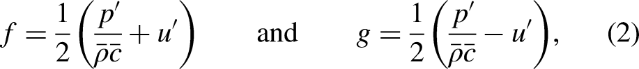
One-dimensional (1D) acoustics, which models the propagation of plane acoustic waves in 1D systems, is described by characteristic wave amplitudes $f$ and $g$ (also called “Riemann invariants” in the mathematical context). We refer to them simply as “acoustic waves” in this work. $f$ and $g$ are related to the primitive acoustic variables $p$ , $u$ , $\rho$ , and $c$ via

$$f=\frac{1}{2}(\frac{p^{\mathrm{\prime }}}{\overline{\rho }\overline{c}}+u^{\mathrm{\prime }})\mathrm{and}g=\frac{1}{2}(\frac{p^{\mathrm{\prime }}}{\overline{\rho }\overline{c}}-u^{\mathrm{\prime }}),$$

(2)

where $p^{\mathrm{\prime }}$ and $u^{\mathrm{\prime }}$ are fluctuations in pressure and velocity and $\overline{\rho }$ and $\overline{c}$ are temporal averaged density and speed of sound, respectively. Conversely, $p^{\mathrm{\prime }}$ and $u^{\mathrm{\prime }}$ are related to $f$ and $g$ by

$$u^{\mathrm{\prime }}=f-g\mathrm{and}{p}^{\mathrm{\prime }}=\overline{\rho }\overline{c}(f+g).$$

(3)

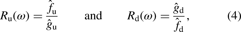
The reflection of acoustic waves at the boundaries (inlet and outlet) is described by the so-called reflection coefficient $R(\omega )$ , which is the ratio of the characteristic wave amplitudes $f$ and $g$

$$R_{\mathrm{u}}\left(\omega \right)=\frac{{\hat{f}}_{\mathrm{u}}}{{\hat{g}}_{\mathrm{u}}}\mathrm{and}{R}_{\mathrm{d}}\left(\omega \right)=\frac{{\hat{g}}_{\mathrm{d}}}{{\hat{f}}_{\mathrm{d}}},$$

(4)

where the subscripts “ $\mathrm{u}$ ” and “ $\mathrm{d}$ ” refer to the upstream (combustor inlet) and downstream boundary (combustor outlet), respectively, and $\widehat{(\cdot )}=(\cdot {)}^{\mathrm{\prime }}{e}^{-i\omega t}$ label variables in the frequency domain assuming harmonic oscillations. The reflection coefficient, which is complex valued, describes the gain and phase between the incident and outgoing acoustic wave. This formalism is suitable only for waves impinging normally to the boundary, which is justified in 1D systems.

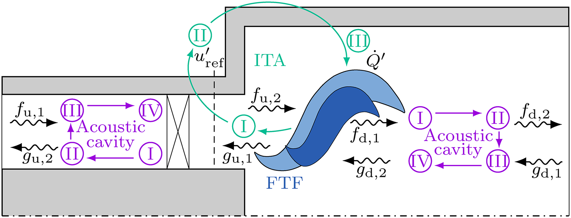
The above described (fully or partially) reflection of acoustic waves at the combustor boundaries closes the so-called outer acoustic loop of the system, shown in violet in Figure 1 for a generic swirl burner. It is explained as follows. First, the flame causes fluctuations in heat release rate (I), which are associated with an unsteady volumetric gas expansion. Such volumetric pulsations generate acoustic waves $g_{\mathrm{u}}$ and $f_{\mathrm{d}}$ traveling upstream and downstream of the flame (II), respectively. The acoustic waves are then reflected at the boundaries (III), depending on the reflection coefficients $R_{\mathrm{u}}$ and $R_{\mathrm{d}}$ . The downstream and upstream traveling reflected acoustic waves $f_{\mathrm{u}}$ and $g_{\mathrm{d}}$ hit the flame (IV) and close the loop. This loop can be also seen as an acoustic cavity (combustor) loop since it depends on the boundaries of the combustor (e.g. open end, choked nozzle, or sinter plate).

Figure 1.

Sketch of plane acoustic wave propagation in a generic swirl burner with (fully or partially) reflecting boundaries. The outer acoustic loop (acoustic cavity) and the internal feedback loop (ITA) are shown in violet and green, respectively. Acoustic cavity: (I) generated acoustic waves $g_{\mathrm{u}}$ and $f_{\mathrm{d}}$ through unsteady volumetric gas expansion, (II) acoustic wave propagation to upstream/downstream boundary, (III) acoustic wave reflection at upstream/downstream boundary, and (IV) acoustic wave propagation of reflected acoustic waves $f_{\mathrm{u}}$ and $g_{\mathrm{d}}$ through the flame; ITA: (I) generated acoustic waves $g_{\mathrm{u}}$ through unsteady volumetric gas expansion, (II) acoustic wave $g_{\mathrm{u}}$ causes acoustic velocity perturbations at the reference position, and (III) acoustic velocity perturbations are coupled with global heat release rate fluctuations via FTF.

An intuitive but invalid point of view, which is still present in the thermoacoustic community, is the following. It is often believed that breaking the acoustic cavity loop, that is, allowing all acoustic waves to leave the domain through the boundaries, leads to a thermoacoustically stable system. A so-called anechoic system is modeled in CFD by incorporating non-reflective acoustic boundary conditions^28,29 ( $R_{\mathrm{u}}=R_{\mathrm{d}}=0$ ). It might be believed that such an anechoic system is unconditionally stable. However, this is a consequence of neglecting the internal acoustic loop, usually known as the intrinsic thermoacoustic (ITA) feedback loop^30–33 (shown in green in Figure 1). The previously described unsteady volumetric gas expansion of the flame (I), produced by the unsteady heat release rate ${\dot{Q}}^{\mathrm{\prime }}$ , causes an acoustic wave $g_{\mathrm{u}}$ to travel in the upstream direction, which in turn modulates the acoustic velocity at the reference position $u_{\mathrm{ref}}^{\mathrm{\prime }}$ (II). These velocity perturbations are coupled via the FTF with fluctuations of global heat release rate ${\dot{Q}}^{\mathrm{\prime }}$ (III), which close the ITA feedback loop. As a result, the stability of a system (as the one depicted in Figure 1) with anechoic boundary conditions is governed by the stability of the ITA loop, as the outer acoustic loop—referred in the following simply as acoustic loop—does not exist for such boundaries. Partially reflecting boundaries, on the other hand, allow both acoustic and ITA loops to co-exist and interact.

It is well known that resonances of acoustic modes lead to peaks in the power spectral distribution of acoustic pressure^34–36. Similarly, it should be clear that resonances of ITA modes may create additional peaks^37,30,38. Importantly, resonances may develop into self-excited instability if any parameter that affects the flame dynamics or the pressure distribution within the system is changed. Examples are fuel composition or inlet/outlet reflection coefficients.

Compressible and incompressible CFD

The main difference between a compressible and incompressible CFD formulation is the absence of acoustic wave propagation in the latter. This absence causes acoustic velocity perturbations associated to dilation mechanisms to be transported instantaneously (i.e. $c\to \mathrm{\infty }$ ) from one point in the domain to another. Acoustic velocity or pressure perturbation upstream of the flame propagate infinitely fast from the inlet to the flame base. Subsequently, the flame base disturbances are convected along the flame. In addition to these convective disturbances, restoration mechanisms ³⁹ —which are a consequence of flame propagation and flame anchoring—are also produced instants after and transported along the flame sheet. The overall fluctuations of the heat release can be thus understood as the flame response to acoustic forcing. Note that in the context of an incompressible formulation, the terminology acoustic perturbation or acoustic forcing can be misleading. In the context of an incompressible simulation in the present paper, such a terminology is exclusively associated with purely axial perturbations that are transported infinitely fast. Note that radial or azimuthal perturbations in the flow, or scalar quantities in general (e.g. temperature), are still transported by convection as in the compressible CFD. Besides the differences in physics, the incompressibility assumption simplifies the numerical setup drastically, since no definition of acoustic boundary conditions is required. Furthermore, acoustic-driven resonances—associated with the acoustic or ITA loop—are avoided.

Acoustic boundary conditions in compressible CFD

To resolve the acoustic wave propagation accurately, special attention goes to the boundary conditions in the compressible CFD, which determine the reflection coefficients defined in equation (4). As discussed above, the intuitive idea of using non-reflective boundary conditions to achieve a thermoacoustically stable system is not generally applicable. Depending on the system under investigation, different combinations of (frequency-dependent) reflection coefficients at the inlet and outlet can lead to a thermoacoustically stable system. This does not necessarily have to be the combination $R_{\mathrm{u}}=R_{\mathrm{d}}=0$ . Therefore, non-reflective boundary conditions should not be always considered optimal acoustic boundary conditions for flame response identification.

A general and very flexible method to prescribe frequency-dependent reflection coefficients $R(\omega )$ is to represent them as a state-space model. These characteristics-based state-space boundary conditions (CBSBC), introduced by Jaensch et al. ²⁹ , are an extension of the partially non-reflective (NSCBC ⁴⁰ ) and fully non-reflective (NSCBC with plane wave masking ²⁸ ) boundary conditions. In the CBSBC framework, the outgoing acoustic wave $f_{\mathrm{d}}$ serves as input to a state-space model that characterizes a linear time-invariant (LTI) system. The following is an example of an outlet boundary:

$$\begin{array}{c}\dot{\mathbf{x}}=A\mathbf{x}+B{f}_{\mathrm{d}},\\ g_{\mathrm{d}}=C\mathbf{x}+Du,\end{array}$$

(5)

with input $f_{\mathrm{d}}$ and output $g_{\mathrm{d}}$ . The system is also characterized by the state vector $\mathbf{x}$ and state-space matrices $A,B,C,D$ . For a given dynamic response of the boundary, the state-space matrices should be evaluated in a calibration step before carrying out CFD ²⁹ .

Different ways of forcing in compressible CFD exist. For example, when considering an inlet boundary, forcing can be performed by imposing either a velocity perturbation (Dirichlet boundary condition, i.e. hard wall) or an acoustic wave via CBSBC condition ¹³ . The latter is used in the present paper because it allows full control of the boundary acoustic reflection. Forcing in the incompressible CFD is done via velocity forcing in the present paper.

System identification

The current paper makes use of the well-established CFD/SI approach ⁴¹ , where high-fidelity CFD is combined with tools from system identification to characterize the response of the flame to velocity perturbations over the entire frequency range of interest with a single broadband-excited CFD simulation. It has to be mentioned that the combustion system under investigation has to be thermoacoustically stable and must not develop resonances or self-excited instability. Otherwise the (linear) SI procedure described in the following should not be applied, since linearity together with time invariance is a prerequisite for the analyzed system ⁴¹ . Once the (thermoacoustically stable) simulation reaches a statistically steady-state after ignition, a broadband signal is imposed at the upstream boundary to generate a time series of acoustic velocity perturbations $u_{\mathrm{ref}}^{\mathrm{\prime }}=[u_0^{\mathrm{\prime }},\dots ,u_N^{\mathrm{\prime }}]$ (input signal) and heat release rate fluctuations ${\dot{Q}}^{\mathrm{\prime }}=[{\dot{Q}}_0^{\mathrm{\prime }},\dots ,{\dot{Q}}_N^{\mathrm{\prime }}]$ (output signal). Input and output signals are then evaluated by correlation analysis, which is a specific kind of system identification ³ .

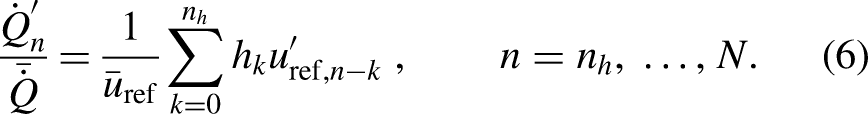
For sufficiently small excitation amplitudes ¹ , the flame response modeled with CFD is considered linear^3,42. It can be modeled by two equivalent approaches: the FTF in the frequency domain (equation (1)) or the finite impulse response in the time domain ⁴¹ . In practice, a finite number of impulse response coefficients $h_k$ give sufficiently accurate results. The finite impulse response is written as

$$\frac{{\dot{Q}}_n^{\mathrm{\prime }}}{\overline{\dot{Q}}}=\frac{1}{{\overline{u}}_{\mathrm{ref}}}\sum _{k=0}^{n_h}{h}_k{u}_{\mathrm{ref},n-k}^{\mathrm{\prime }},n=n_h,\dots ,N.$$

(6)

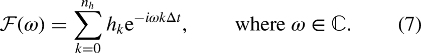
The impulse response is typically not known a priori and has to be estimated from time series data $u^{\mathrm{\prime }}$ and ${\dot{Q}}^{\mathrm{\prime }}$ via an optimal linear least square estimator ³ , known as the Wiener-Hopf equation. For more information see Silva et al. ³⁸ , Since the unit impulse response and FTF are fundamentally equivalent, they can be converted into each other via z-transform

$$\mathcal{F}\left(\omega \right)=\sum _{k=0}^{n_h}{h}_k{\mathrm{e}}^{-i\omega k\mathrm{\Delta }t},\mathrm{where}\omega \in \mathbb{C}.$$

(7)

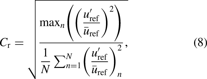
The signal used for perturbing the flame over a large range of frequencies has to fulfill specific quality criteria. One of them is the crest factor

$$C_{\mathrm{r}}=\sqrt{\frac{\underset{n}{max}\left({\left(\frac{u_{\mathrm{ref}}^{\mathrm{\prime }}}{{\overline{u}}_{\mathrm{ref}}}\right)}^2\right)}{\frac{1}{N}\sum _{n=1}^N{\left(\frac{u_{\mathrm{ref}}^{\mathrm{\prime }}}{{\overline{u}}_{\mathrm{ref}}}\right)}_n^2},}$$

(8)

which relates the ratio of the largest absolute value of the signal to the root mean square (RMS) value of it. The crest factor is one of the most important quality measures in signal processing with a theoretical optimum of unity ³ . This value is desirable to avoid outlier peaks in the time series, as they can trigger nonlinear mechanisms in the response. A discrete random binary signal (DRBS), for example, has a maximum utilization of the signal power due to binary amplitudes of either 1 or $-1$ , which leads to $C_{\mathrm{r}}=1$ .

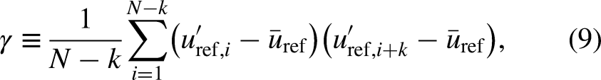
Another quality measure of interest evaluates the level of correlation of the signal with itself, namely autocorrelation, estimated as follows^43,41,44

$$\gamma \equiv \frac{1}{N-k}\sum _{i=1}^{N-k}(u_{\mathrm{ref},i}^{\mathrm{\prime }}-{\overline{u}}_{\mathrm{ref}})(u_{\mathrm{ref},i+k}^{\mathrm{\prime }}-{\overline{u}}_{\mathrm{ref}}),$$

(9)

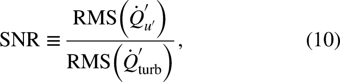
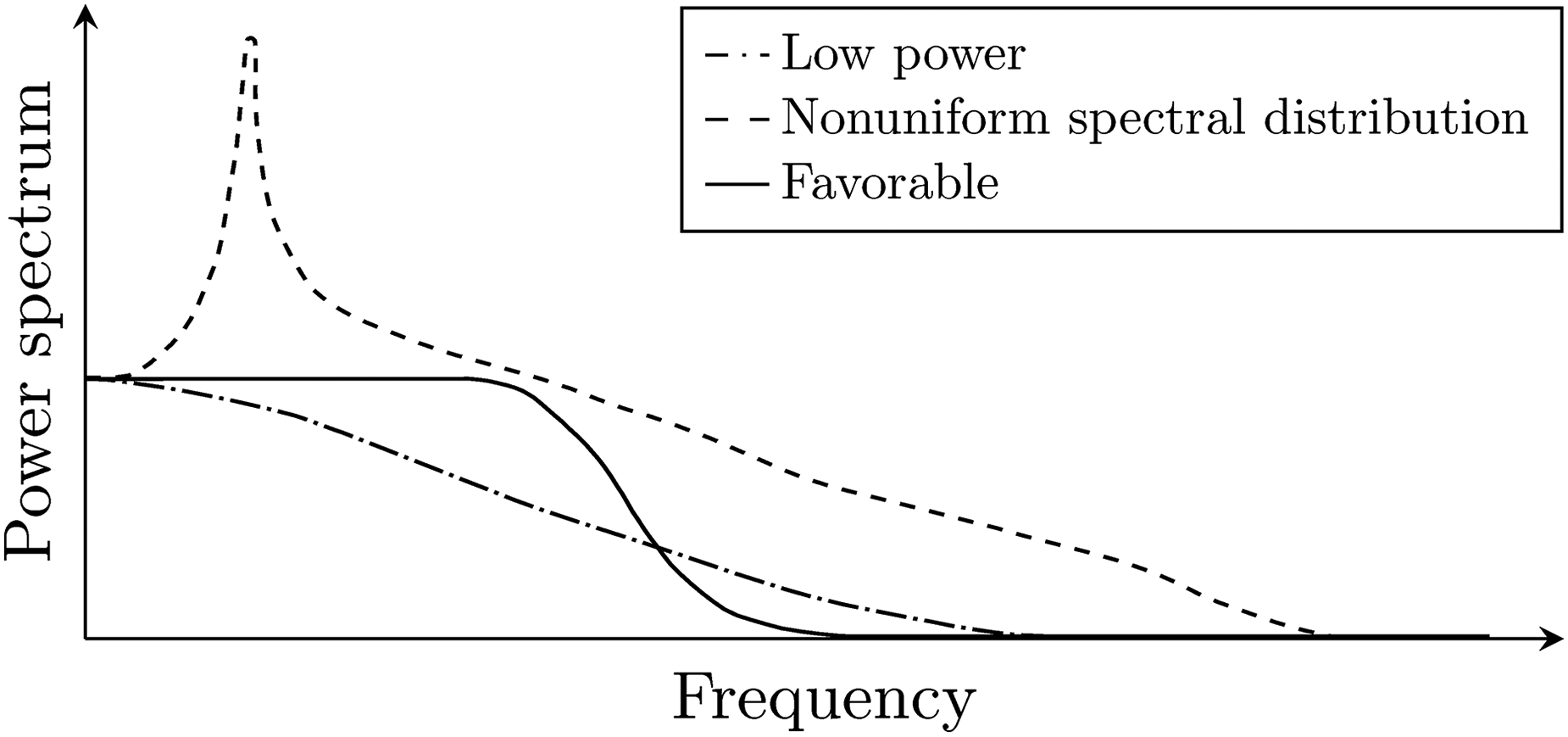
where $k$ is a certain time lag. Low values of $\gamma$ result in high statistical independence. Furthermore, a good signal typically shows broadband, low-pass filtered spectral characteristics with uniform amplitude in the frequency range of interest ⁴⁵ (see black curve in Figure 2). In systems with noise, low power (see dash-dotted curve in Figure 2) may lead to poor identification quality, mainly because of a low signal-to-noise ratio (SNR). SNR is defined as ⁴⁶

$$\mathrm{SNR}\equiv \frac{\mathrm{RMS}\left({\dot{Q}}_{u^{\mathrm{\prime }}}^{\mathrm{\prime }}\right)}{\mathrm{RMS}\left({\dot{Q}}_{\mathrm{turb}}^{\mathrm{\prime }}\right)},$$

(10)

where ${\dot{Q}}_{u^{\mathrm{\prime }}}^{\mathrm{\prime }}$ denotes the heat release rate fluctuations resulting purely from acoustic excitation and ${\dot{Q}}_{\mathrm{turb}}^{\mathrm{\prime }}$ stands for the heat release rate fluctuations produced by turbulence (variance of pure noise). From equation (10) it might be concluded that a high SNR (and therefore high forcing amplitudes) is appropriate for CFD/SI, as long as a nonlinear response is not triggered. Note that peaks in the amplitude content (which lead to high SNR) can trigger nonlinear flame behavior at specific frequencies (see dashed curve in Figure 2). Note also that a proper signal exhibits a uniform amplitude spectrum along the frequency band of interest (see the solid curve in Figure 2), resulting in an uniform SNR per frequency. This uniform distribution of SNR is desirable, since the influence of noise can be considered similar within the frequency band of interest.

Figure 2.

Power spectrum of three different broadband signals. Examples of a low power signal, a signal with nonuniform spectral distribution, and a favorable signal.

Turbulent premixed swirl burner

Experimental setup

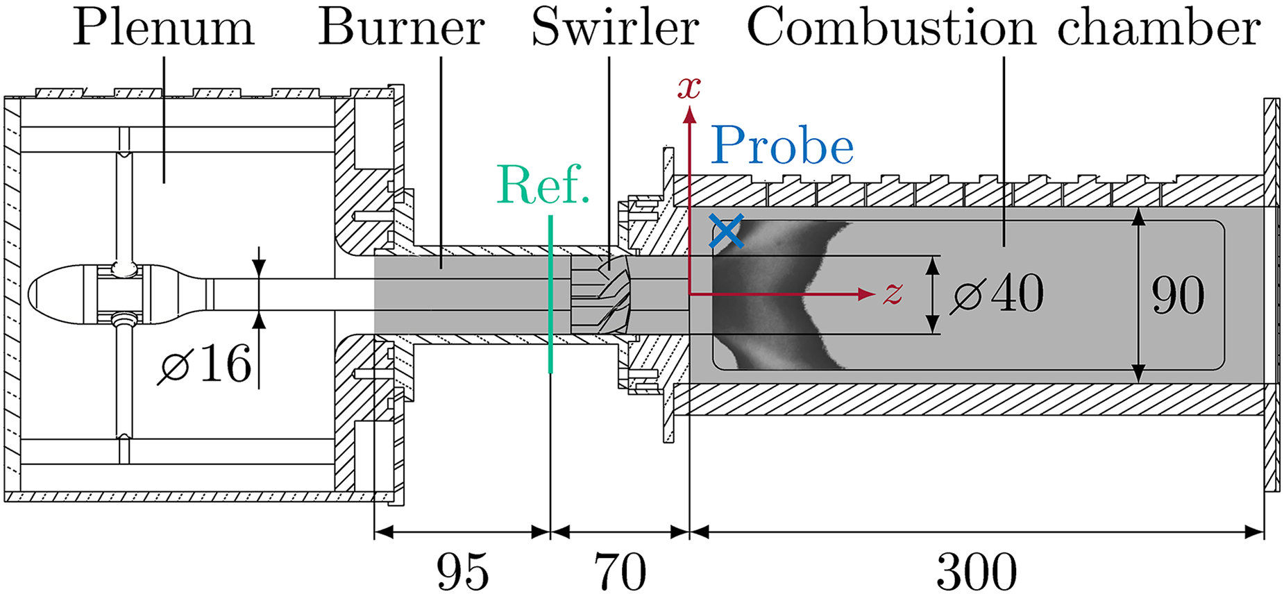
In the present work, the turbulent swirl-stabilized laboratory-scale combustor shown in Figure 3 is studied for the comparison of compressible and incompressible LES. The perfectly premixed BRS burner test rig includes an axial swirl generator with eight vanes mounted on a central bluff body, which is characterized by a theoretical swirl number $S=0.74$ ⁷ . The circular plenum is located upstream of an annular flow passage (called burner). The squared combustion chamber downstream of the burner features two quartz glass windows for chemiluminescence measurements and houses a perforated plate at the combustor outlet. The swirler position near the burner outlet results in a small pressure drop between the swirler and combustion chamber, which means that the swirler can be considered acoustically transparent ⁴⁷ .

Figure 3.

Experimental setup of the BRS burner ⁷ test rig with a pressure probe located at (40 0 15) mm. The shaded area represents the part resolved with LES. Dimensions are given in mm.

The burner was developed and experimentally investigated by Komarek and Polifke ⁷ . It was operated under perfectly premixed conditions of methane and air. The experimental data in the present work always refers to the $30\mathrm{kW}$ thermal power rating and $\varphi =0.77$ equivalence ratio configuration. OH ${}^{*}$ chemiluminescence was measured with an intensified CMOS camera. ⁷ A recorded time of about $4\mathrm{s}$ was averaged to determine the steady-state average of OH* emissions. The velocity signal at the reference position was obtained by Constant Temperature Anemometry (CTA) measurements. Compressible LES with AVBP^9,48, and incompressible LES with Fluent^19,20 and OpenFOAM 5.x ²¹ of the BRS burner were carried out in previous studies on the dynamics of premixed flames. Both incompressible and compressible studies showed good agreement of the predicted FTF when compared with experimental data.

Numerical setup

Large eddy simulations using the open source C++ library OpenFOAM 5.x ⁴⁹ are performed. The fully compressible Navier-Stokes equations using the reactingFoam solver are solved, where the density is a function of temperature and pressure $\rho (T,p)$ . For the incompressible simulation, the original solver was customized for the treatment of incompressible flows, where the density is only a function of the temperature $\rho (T)$ ²¹ . In terms of implementation, the pressure is split into a hydrodynamic pressure and a constant thermodynamic pressure ⁵⁰ . Kinetic energy terms and the mechanical work term $\frac{\mathrm{\partial }p}{\mathrm{\partial }t}$ are removed from the energy equation. Other terminologies like “low Mach number” or “weakly-compressible” formulations are also common for such incompressible solvers, where the acoustics are effectively removed from the governing equations ²² . With the approximation that density is only a function of temperature, an incompressible solver can still capture the time-averaged flame shapes and flow fields of a thermoacoustically stable condition as validated in previous studies^24,51,19 and also shown in section “Unforced flow/flame validation.”

The shaded area in Figure 3 represents the numerical domain resolved in the LES with a reference position for the FTF identification as in the experiment at $z=-70$  mm. The CFD/SI approach does not require resolving the whole combustion system. Therefore, in order to reduce computational costs ⁴¹ , only the vicinity of the flame has to be resolved in the simulation, whereas the effect of the system boundaries may be considered by impedance boundary conditions (e.g. CBSBC). For system identification, these do not have to be realistic, but must ensure a thermoacoustically stable configuration.

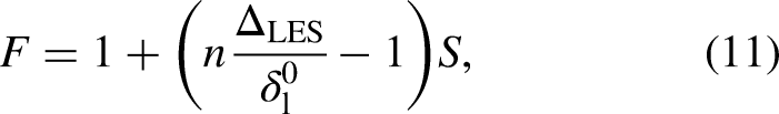
The governing equations are solved on an unstructured grid consisting of approximately 5 million cells (predominantly hexagonal) with refinement zones in the swirler and flame region. A typical cell size in the latter is $500$ – $600\mu \mathrm{m}$ , which is close to the laminar flame thickness of about $460\mu \mathrm{m}$ . In terms of Pope’s criterion ⁵² , over 90% of the turbulent kinetic energy are resolved as shown in a previous study ²¹ . Similarly, a grid independence study was previously performed ²¹ . A fully implicit second-order accurate Euler scheme is used, which was found to be sufficient for CFD/SI ⁴¹ . The time step is fixed at $\mathrm{\Delta }t=1\times {10}^{-6}$ s for both simulations, which yields a maximum hydrodynamic CFL number of 0.3. A PIMPLE-consistent algorithm (with three outer iterations) is employed to solve the pressure–velocity coupling in the compressible simulation without being restricted by the acoustic CFL number, and PISO-consistent is used in the incompressible case (both use three inner iterations). The additional three outer iterations increase the runtime of the compressible LES by almost this factor. The wall-adapting local eddy-viscosity (WALE) sub-grid model ⁵³ without using a wall function is applied to close the Favre-filtered Navier-Stokes equations of mass, momentum, species mass fraction, and energy at atmospheric conditions. An extended version of the dynamic thickened flame model^54–57, with local sensor $S$ and an efficiency function, is used to take turbulence-flame interaction into account. The dynamically thickened flame front is resolved with $n=7$ cells and a maximum thickening factor $F_{\max }<10$ is kept ⁵⁶ . The thickening factor is defined as

$$F=1+(n\frac{{\mathrm{\Delta }}_{\mathrm{LES}}}{{\delta }_{\mathrm{l}}^0}-1)S,$$

(11)

where ${\mathrm{\Delta }}_{\mathrm{LES}}$ is the LES filter width and ${\delta }_{\mathrm{l}}^0$ is the laminar flame thickness defined from the temperature profile gradient ⁵⁵ . The thickened flame model is not affected by the choice of compressible or incompressible solvers ⁵⁸ . The chemical reactions are modeled with the two-step global mechanism 2S_CH4_BFER by Franzelli and Riber ⁵⁹ . The species and energy equations are modeled with unity Lewis number and Schmidt number $Sc=0.7$ for all species, which is a common approximation for hydrocarbon combustion ⁶⁰ .

For the identification of flame dynamics, a frequency-limited (1000 Hz) Daubechies wavelets-based signal (DWBS) ⁴⁵ is imposed at the upstream end of the computational domain. The cut-off frequency $f_{\mathrm{cut}}\approx 630$  Hz and a constant amplitude spectrum up to around $500$  Hz (maximum frequency of interest in the present study) is achieved. The maximum amplitude of the signal is 10% of the mean inlet velocity ${\overline{u}}_{\mathrm{inlet}}=11.3$  m/s. A similar excitation amplitude has shown linear flame response in previous studies of the swirl-stabilized BRS burner^19,21. Note that identical signals were used for the compressible and incompressible LES.

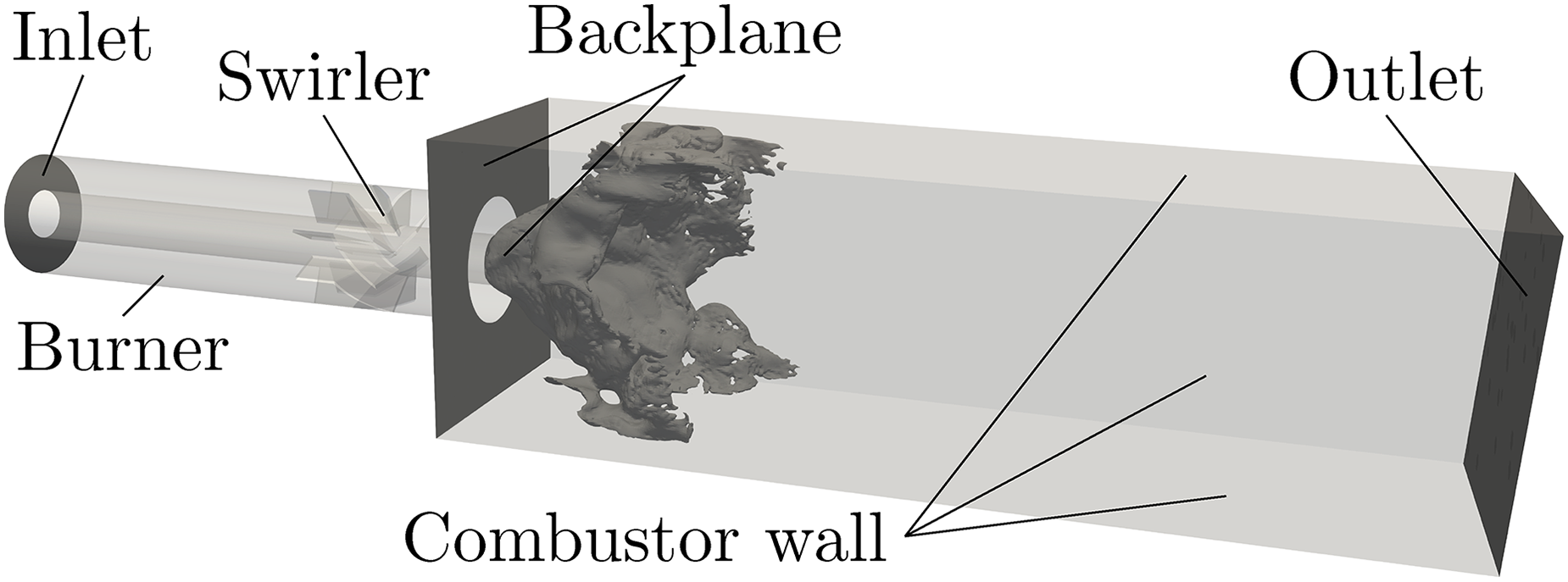
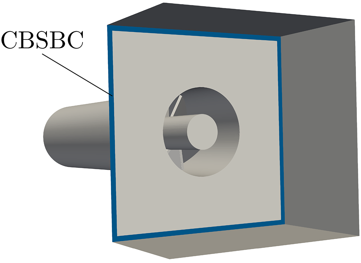
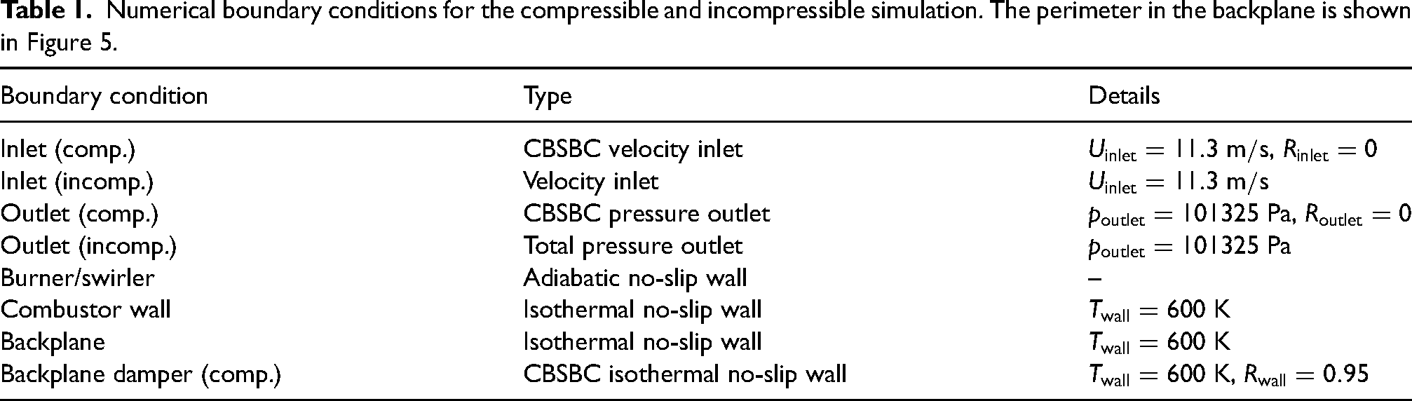
The boundary conditions are shown in Figure 4 and indicated in Table 1. The combustor walls and the bluff body plane are set to no-slip isothermal walls with a fixed temperature of $600\mathrm{K}$ . The combustor wall temperature is an estimated value based on measurements of a similar burner configuration as mentioned in Tay-Wo-Chong et al. ⁴⁸ , Previous studies^61–63 show that wall heat transfer in the combustion chamber is very important for correct modeling of the flame shape (and therefore the flame dynamics) in swirl-stabilized combustors. Uncertainty in wall temperature in the experiment might cause deviations in the flame response evaluation with LES ⁶⁴ . The burner section including the swirler is treated as an adiabatic no-slip wall, which is sufficient as the reaction only takes place inside the combustion chamber. CBSBC are used for the compressible LES due to the advantages discussed in section “Modeling approaches”. To overcome an unstable transverse chamber mode in the compressible LES, CBSBC with a reflection coefficient near one ( $R_{\mathrm{wall}}=0.95$ ) is used at a small outer slit of the backplane to suppress the amplifying mode, as shown in Figure 5. The results of the simulation with and without transverse mode damping are properly discussed in section “Unforced flow/flame validation.” After an iterative “trial and error” procedure with different combinations of upstream and downstream reflection coefficients ² , the use of non-reflective boundaries at the inlet and outlet turned out to be a good choice, as they assure in the present case thermoacoustic stability.

Figure 4.

Numerical setup and boundary conditions of the BRS burner. The flame is visualized by an iso-surface of the ${\mathrm{CH}}_4$ concentration.

Figure 5.

Unstable transverse mode is suppressed with an impedance boundary condition (CBSBC) imposed at the perimeter (blue) of the combustion chamber backplane.

Table 1.

Numerical boundary conditions for the compressible and incompressible simulation. The perimeter in the backplane is shown in Figure 5.

Boundary condition	Type	Details
Inlet (comp.)	CBSBC velocity inlet	$U_{\mathrm{inlet}}=11.3\mathrm{m}/\mathrm{s}$ , $R_{\mathrm{inlet}}=0$
Inlet (incomp.)	Velocity inlet	$U_{\mathrm{inlet}}=11.3\mathrm{m}/\mathrm{s}$
Outlet (comp.)	CBSBC pressure outlet	$p_{\mathrm{outlet}}=101325\mathrm{Pa}$ , $R_{\mathrm{outlet}}=0$
Outlet (incomp.)	Total pressure outlet	$p_{\mathrm{outlet}}=101325\mathrm{Pa}$
Burner/swirler	Adiabatic no-slip wall	–
Combustor wall	Isothermal no-slip wall	$T_{\mathrm{wall}}=600\mathrm{K}$
Backplane	Isothermal no-slip wall	$T_{\mathrm{wall}}=600\mathrm{K}$
Backplane damper (comp.)	CBSBC isothermal no-slip wall	$T_{\mathrm{wall}}=600\mathrm{K}$ , $R_{\mathrm{wall}}=0.95$

Unforced flow/flame validation

Unstable transverse mode in the compressible LES

A transverse mode at approximately $f=4170$  Hz develops in the combustion chamber during unforced compressible simulations as shown in Figure 6. The mode matches with the first transverse eigenmode of the combustion chamber $f_{1\mathrm{T}}=\frac{c}{2H}=4139$  Hz, where $H=0.09$  m and $c={\overline{c}}_{\mathrm{chamber}}=745$  m/s. This high-frequency instability is self-exciting and was not observed in the experiments, but similar observations were made in previous numerical studies.^48,65,66 Several types of initialization were tested, but the instability developed regardless of the procedure used. Therefore, it is concluded that the unstable mode is not a numerical instability, but physically correct in an acoustically ideal environment such as a computational domain. On the other hand, quartz windows are not perfectly sealed (i.e. there is leakage of combustion chamber) and geometry features in the experiment are not ideal compared to a numerical model: corners are not perfectly sharp and chamber walls exhibit certain roughness, which enhance acoustic dissipation. Such additional losses might explain why the mode was not observed in experiments.

Figure 6.

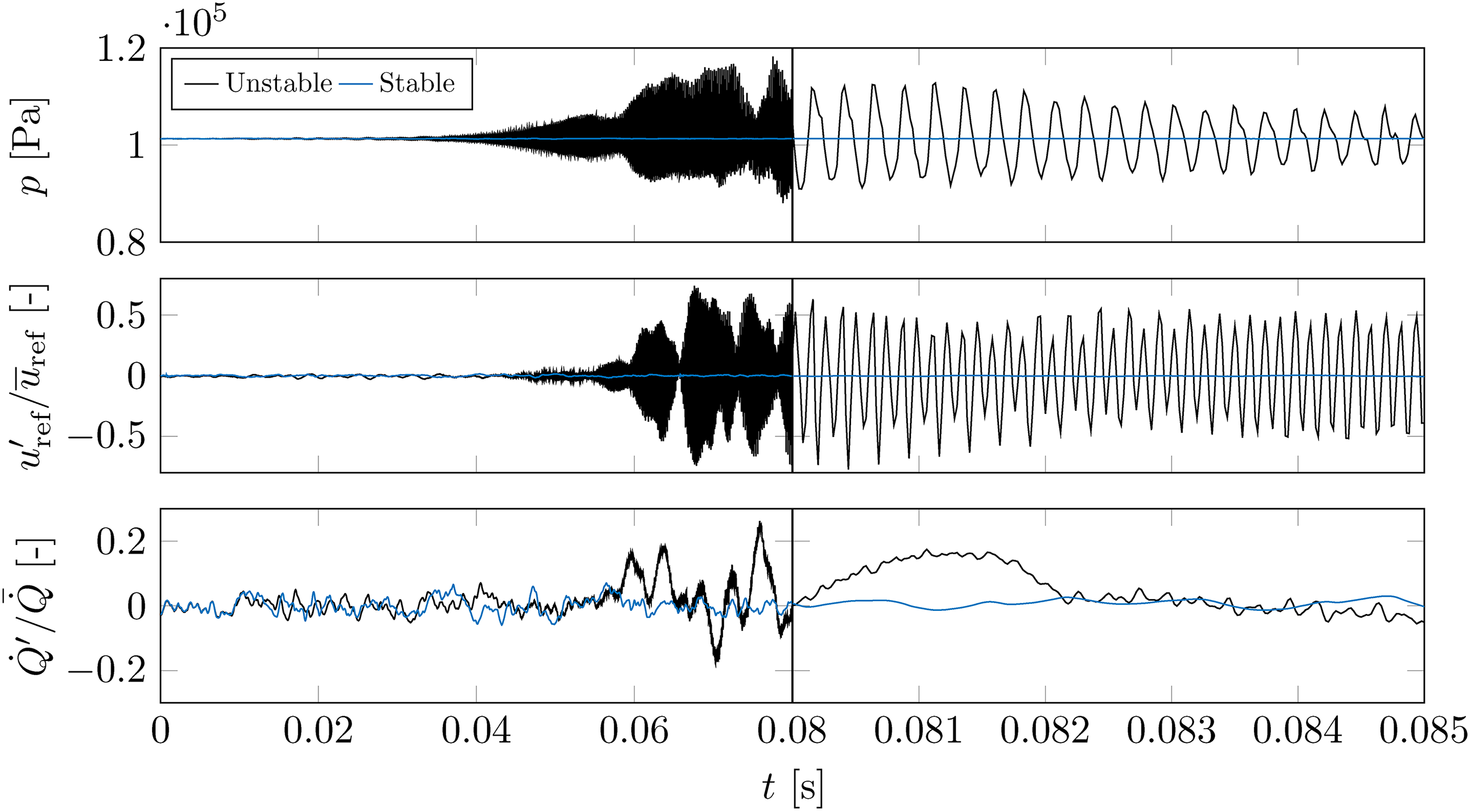
Pressure fluctuation (top), input velocity signal (middle) and output heat release rate signal (bottom) of the unstable and stable compressible LES. Pressure probe is located at $(40015)$ mm in the combustion chamber (illustrated in Figure 3). Note the non-equidistant time axis.

Figure 6 shows that the pressure perturbations start to increase after around $30$  ms and continue increasing up to a limit cycle. The pressure is measured on a probe located at (40 0 15) mm, illustrated in Figure 3. Velocity perturbations are slightly affected once the pressure perturbations start to increase. Velocity amplitudes reach up to $50\text{\%}{\overline{u}}_{\mathrm{inlet}}$ . Similarly, the global heat release rate is also affected, as the high-frequency instability affects the shape and overall dynamics of the flame. The measured input and output signals are thus corrupted and cannot be used for system identification.

In order to suppress the high-frequency instability, the acoustic behavior of the four chamber walls was originally manipulated, where a reflection coefficient near one ( $R_{\mathrm{wall}}=0.95$ ) was imposed with the CBSBC method. A similar approach with “soft NSCBC” walls was presented and applied by Ghani et al. ⁶⁶ . However, in the present case, this approach turned out to influence the flame dynamics, as observed with harmonic analysis and broadband SI (not shown in the present paper). It was concluded that such an approach is not adequate for later flame dynamics analysis and is therefore not used in the present study.

The selected damping approach is the following. The outlet formulation of CBSBC with $R_{\mathrm{wall}}=0.95$ is imposed at the perimeter of the combustion chamber backplane, as shown in Figure 5. An acoustic slit with a width of four numerical cells, where only acoustic flux is allowed, turned out to sufficiently suppress the transverse mode without influencing the flame dynamics, as analyzed by several harmonically excited simulations (not shown in the present paper). With the reflection coefficient close to unity, the slot is slightly acoustically softer than the rest of the (acoustically hard) combustor wall. The excellent performance of this arrangement is shown in Figure 6 (blue). This damping strategy was inspired by the ones used in industrial gas turbines ⁶⁷ . Compared to the latter, which considers Helmholtz or quarter-wave resonators, we do not use holes in the backplane, but an acoustic slit in order to avoid influencing the flow field.

Comparison of time-averaged flow/flame quantities in the compressible and incompressible LES

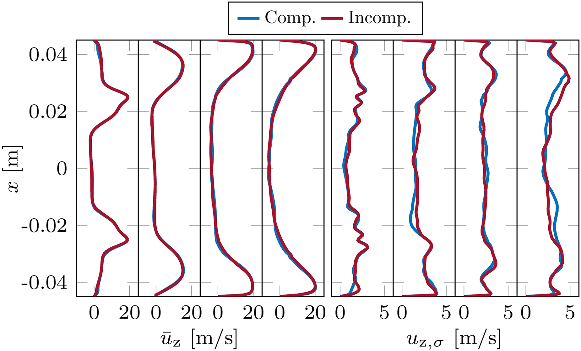
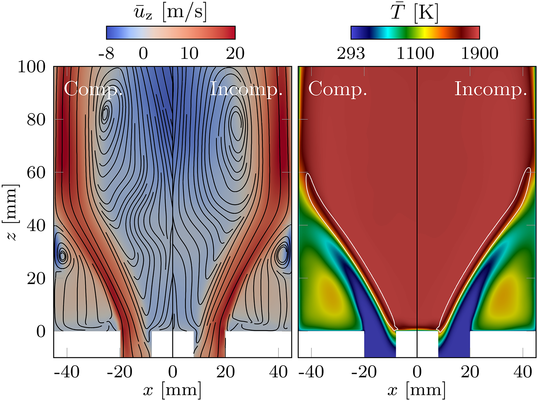
An obligatory test for the correctness of a CFD simulation is the comparison of velocity profiles at different axial positions. The associated time-averaging was carried out over $100$  ms in the compressible and incompressible cases. Profiles of time-averaged and RMS axial velocity components at different positions downstream the combustion chamber entry are compared, as illustrated in Figure 7. The RMS velocity is calculated as $u_{\mathrm{z},\sigma }=\sqrt{\overline{u_{\mathrm{z}}^{{\mathrm{\prime }}^2}}}$ = $\sqrt{\frac{1}{N}\sum _i^N(u_{\mathrm{z}}-{\overline{u}}_{\mathrm{z}}{)}^2}$ , where $N$ is number of samples for time averaging. Note that the comparison is limited to CFD, as no velocity measurements (PIV) are available for the $30$ kW thermal power configuration ²⁰ . Therefore, due to the lack of experimental data of velocity for the present case, the prediction of flame-turbulence interaction cannot be considered fully validated. However, the agreement between compressible and incompressible LES is very good. Time-averaged axial velocity and temperature fields of both LES are shown in Figure 8 together with surface streamlines and iso-contours of the heat release rate, respectively. The velocity fields show classical flow features of a swirl burner, namely a strongly pronounced central recirculation zone (CRZ) downstream of the bluff body and a weaker outer recirculation zone (ORZ) typical for V-shaped flames. The flame shapes are also present in the temperature fields, which exhibit relatively low temperatures in the ORZ compared to the burnt gases. Overall, both fields are in good agreement in the LES.

Figure 7.

Profiles of time-averaged (left) and RMS (right) axial velocity components of compressible and incompressible LES at various measurement planes ( $z$ =20, 40, 60 and 80 mm) downstream of the combustion chamber entry.

Figure 8.

Time-averaged fields of axial velocity with surface streamlines (left) and temperature (right) of compressible and incompressible LES. White iso-contours refer to the heat release rate of level $2\times {10}^8$  W/m ${}^3$ .

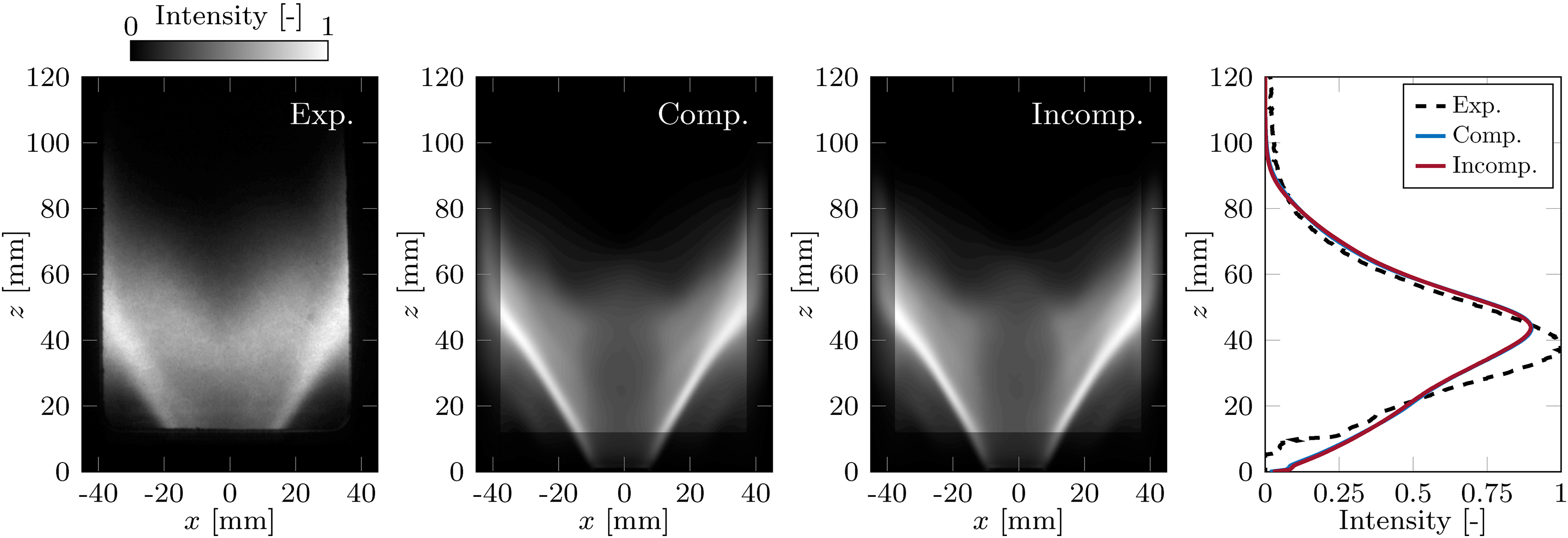
Time-averaged heat release rate fields from both simulations were line-of-sight (LOS) integrated along the width of the combustion chamber. A comparison between time-averaged OH ${}^{*}$ chemiluminescence emission measurements from the experiment and the normalized heat release rate from LES is feasible because heat release rate $\dot{Q}$ is proportional to light emission intensity of OH ${}^{*}$ in perfectly premixed systems ⁶⁸ . Figure 9 shows the spatial distribution of the normalized (with its maximum) time-averaged OH ${}^{*}$ chemiluminescence emission measurements from the experiment and the normalized heat release rate from LES. The cage of the combustion chamber, where the quartz windows are mounted, is represented with a shaded area in the images of the simulations. The flame angle at the bluff body, as well as the flame length, is correctly reproduced in both LES. Each flame shows the characteristic stabilization in the inner shear layer only, which is known as a “V-shaped” flame. Capturing the flame length and shape are essential features for the correct identification of flame dynamics ⁶⁹ .

The simulated flame shapes stand in good agreement with that of the experiment and no differences between the compressible and incompressible LES are visible. The heat release rate distributions of LES are normalized with the area under the curve of the experimental distribution (reference area) since the amount of burnt fuel (or produced heat release) in experiments and simulations should be equivalent. The agreement between the experiment and LES is very good from approximately $0.045$ m behind the chamber entry (see Figure 9 right). A possible reason for the mismatch at the burner outlet is the missing optical access in the experimental setup. This would explain the zero value until $0.01$  m. The heat release at the burner mouth is higher in LES, whereas the OH ${}^{*}$ chemiluminescence emissions could not be measured directly at the bluff body plane, because the cage of the quartz windows limited the view field of the camera. For a better agreement in the close vicinity of the combustion chamber entry, a more advanced modeling approach for the wall temperature boundary conditions (i.e. conjugate heat transfer) at the backplane has to be used in LES^62,63. However, a correct modeling is very challenging because there is no reliable data on wall temperatures from the experiment. In any case, the agreement between compressible and incompressible LES is excellent, which is of higher priority than agreement with the experiment in the present study.

Figure 9.

Comparison of experimental time-averaged LOS integrated OH ${}^{*}$ chemiluminescence image with time-averaged LOS integrated heat release rate field $\overline{\dot{Q}}$ from compressible and incompressible LES. The normalized spatial distribution of heat release rate from experiment, compressible and incompressible LES is shown in addition. Note that the blue and red lines overlap.

Flame response to velocity perturbations of the premixed swirl burner

Since the steady-state results shown in the previous section match very well, the corresponding flame dynamics is analyzed in this section. Compressible and incompressible LES are excited with broadband signals to identify with one simulation the flame response over the frequency range up to $500$  Hz. The compressible LES is forced with an acoustic wave $f_{\mathrm{ex}}$ and the incompressible LES is forced with an acoustic velocity perturbation $u_{\mathrm{ex}}^{\mathrm{\prime }}$ , where the subscript “ $\mathrm{ex}$ ” stand for excitation. Both methods are compared directly with each other and validated with experimental data. For additional numerical validation, results from harmonic excitation at specific frequencies are used. First, the quality of the generated time series data is evaluated. Afterwards, the FTF is identified with harmonic analysis and a finite impulse response model.

Evaluation of input and output signals

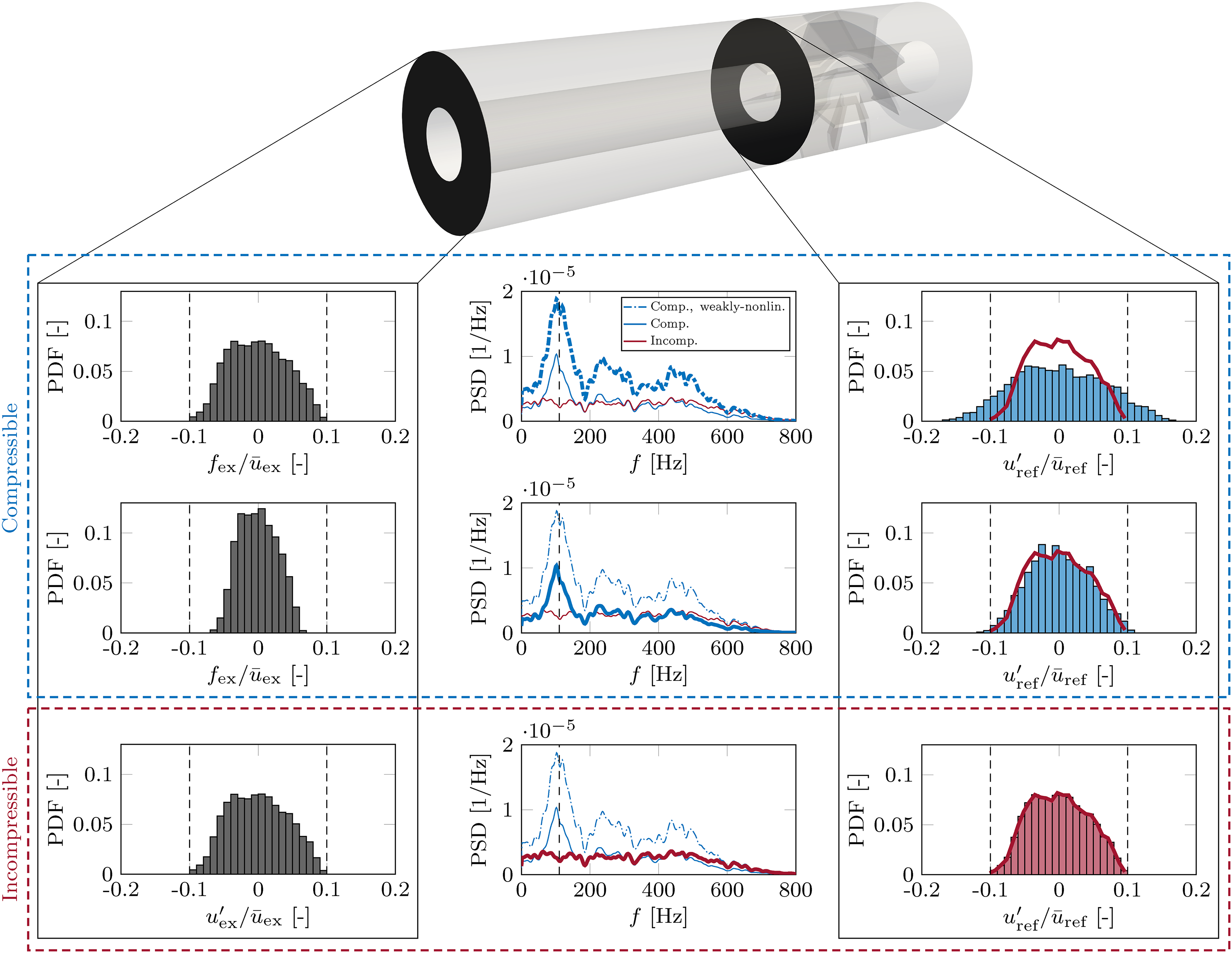
As stated above, compressible and incompressible LES are excited with a broadband signal with maximum amplitude $f_{\mathrm{ex}}/{\overline{u}}_{\mathrm{ex}}=0.1$ (compressible) and $u_{\mathrm{ex}}^{\mathrm{\prime }}/{\overline{u}}_{\mathrm{ex}}=0.1$ (incompressible) in order to generate time series for subsequent system identification. The probability density function (PDF) of both excitation signals is shown in Figure 10 (left column). In a turbulent flame, the amplitude of the excitation signal has a significant effect on the identification of flame dynamics, even in the linear flame regime. If the excitation amplitude is chosen too low, the SNR (excitation signal compared to turbulent noise) is too low and a clear identification of the FTF is no longer possible. Therefore, the amplitude has to be chosen such it assures linear flame behavior on the one hand and keeps the SNR high enough for an accurate system identification procedure on the other. The amplitudes $f_{\mathrm{ex}}/{\overline{u}}_{\mathrm{ex}}=0.1$ (compressible) and $u_{\mathrm{ex}}^{\mathrm{\prime }}/{\overline{u}}_{\mathrm{ex}}=0.1$ (incompressible) are selected, as illustrated in Figure 10.

Figure 10.

Influence of intrinsic thermoacoustic (ITA) feedback loop on input signal. Left column: PDF of excitation signals (imposed at inlet boundary). Middle column: PSD of weakly-nonlinear compressible, compressible and incompressible LES . Note hat the same three PSDs are shown in each figure in the middle column for comparison purposes. The thick line highlights the case that corresponds to each row (top: weakly-nonlinear compressible; middle: compressible; bottom: incompressible). Right column: PDF of input signals (evaluated at reference position) with PDF of incompressible LES (solid, red) as comparison.

Note that it is not the amplitude of the excitation signal (imposed at the inlet boundary), but the amplitude of the velocity perturbations at the reference position (input signal) what is of primary interest for flame perturbation and also FTF identification. The PDF of the compressible and incompressible input signal is shown in Figure 10 (right column), where the incompressible PDF is marked as reference. Note that, in contrast to the incompressible case, the input signal in the compressible case—and therefore the associated PDF—is different from its corresponding excitation signal. Differences between the excitation and input signals in the compressible LES are also observed with the power spectrum of the latter, shown in the middle column in Figure 10. Its peaks at three specific frequencies (110 Hz, 260 Hz and 470 Hz) are a manifestation of resonances within the system. The dominant peak at $f_{\mathrm{PSD},1}$ is associated with the first ITA mode of the anechoic BRS burner, identified with the $-\pi$ criterion from the FTF shown in Figure 13. The intrinsic thermoacoustic feedback loop, explained in section “Modeling approaches”, causes a resonance in the system, which is clearly observed in the power spectrum. Such high resonances cause significant differences between excitation and input signals. Note that the flame does not respond to the imposed excitation signal, but to the input signal extracted upstream of the flame. The disparity between the two signals must be taken into account during pre-processing when generating an excitation signal. It may be necessary to iteratively modify the excitation signal until the input signal exhibits the desired features.

Figure 13.

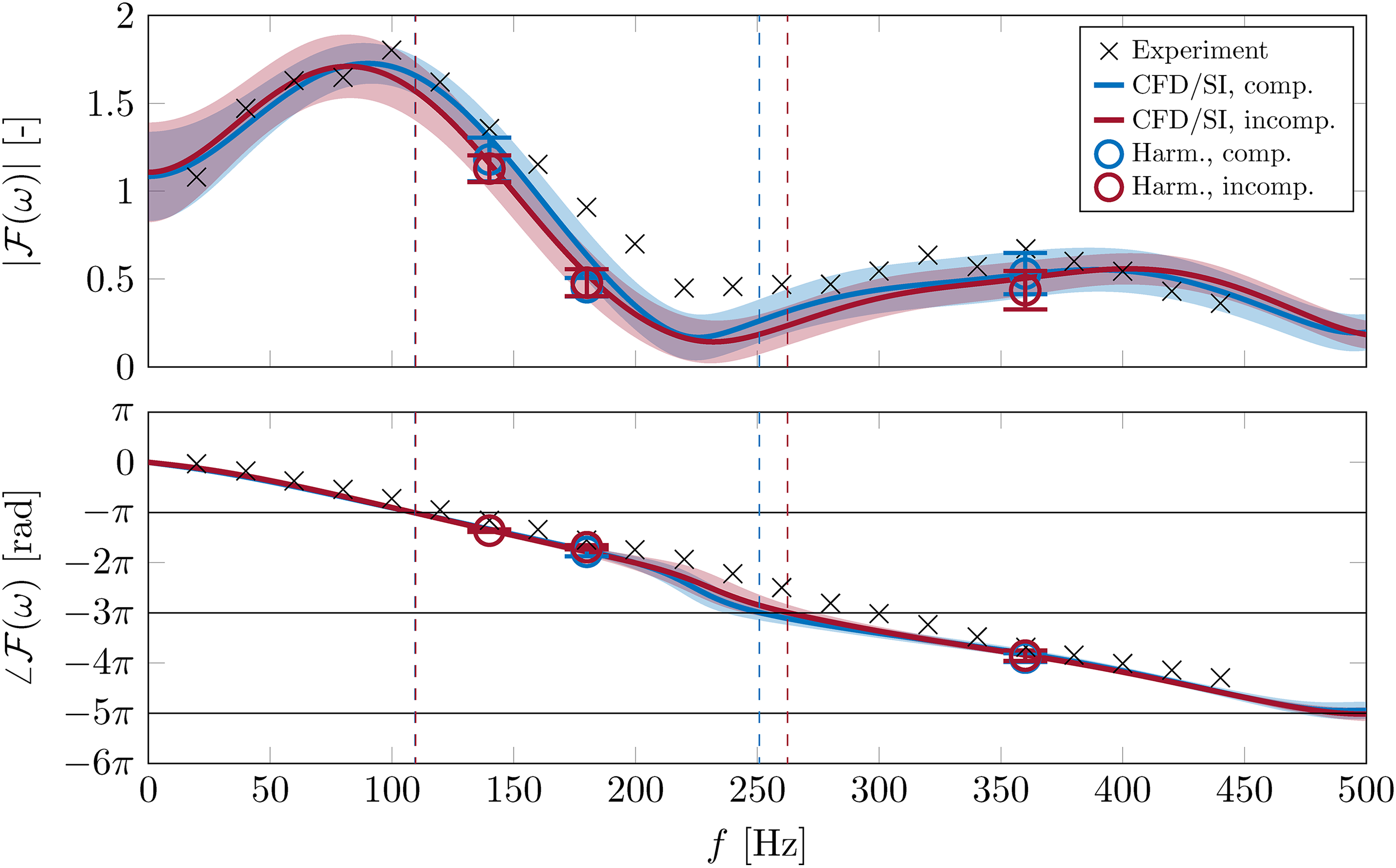
Frequency response from experiment, compressible CFD/SI and incompressible CFD/SI with the respective $\sigma =1.96$ confidence intervals. Vertical lines (solid, black) indicate ITA frequencies according to the $-\pi$ criterion for the compressible (dashed, blue) and incompressible (dashed, red) case.

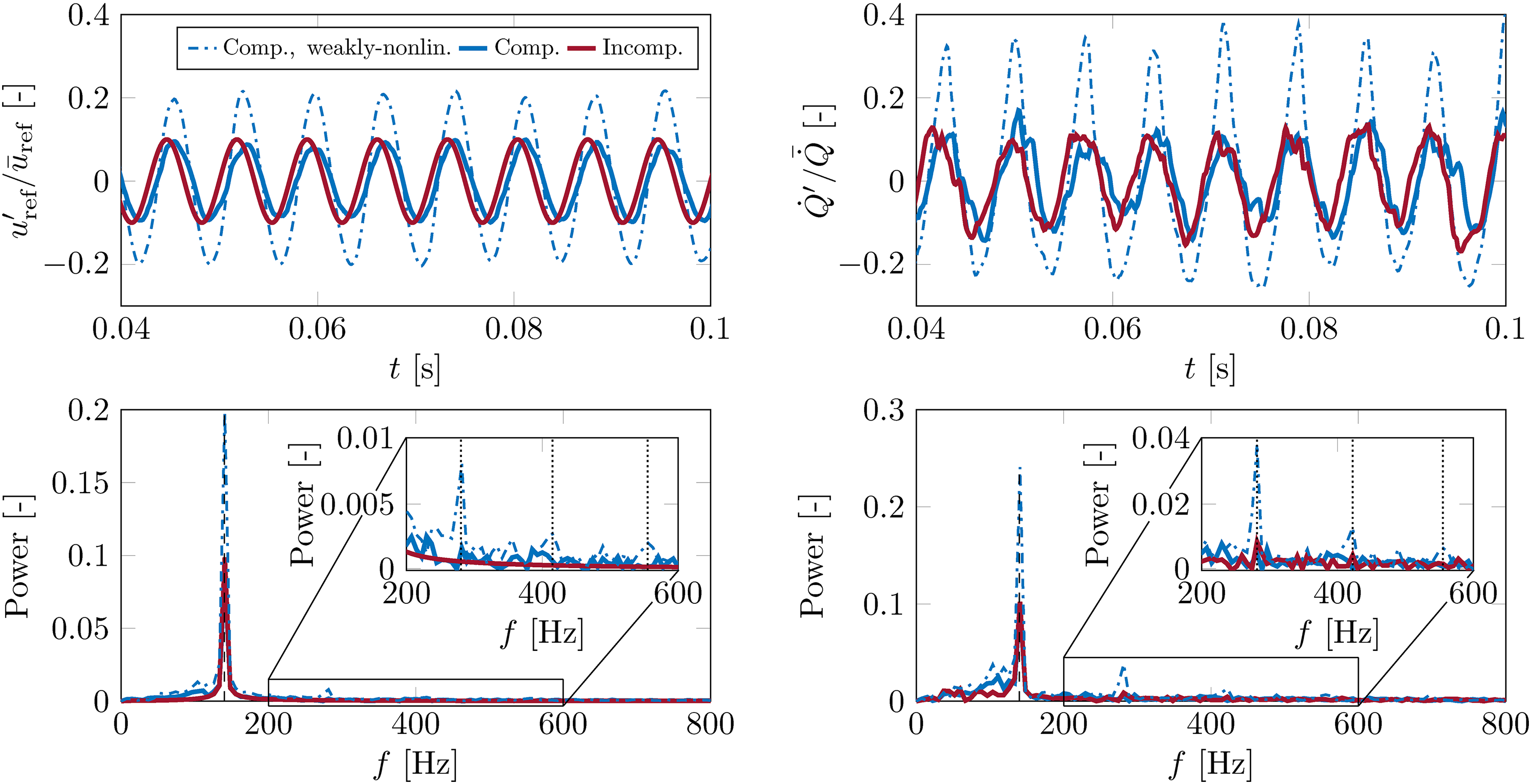
A strong ITA resonance as shown in Figure 10 (middle column) is linked to high amplitudes of the $g$ wave, which is simply explained with equation (3). In the specific case of $f_{\mathrm{ex}}/{\overline{u}}_{\mathrm{ex}}=0.1$ , this leads to maximum amplitudes of the input signal up to $u_{\mathrm{ref}}^{\mathrm{\prime }}/{\overline{u}}_{\mathrm{ref}}>0.17$ , which may cause a nonlinear flame response that cannot be investigated by linear identification models. To check nonlinearity of the compressible LES, a harmonic excitation at $140$  Hz is used. The amplitude of the excitation signals is again $f_{\mathrm{ex}}/{\overline{u}}_{\mathrm{ex}}=0.1$ (compressible) and $u_{\mathrm{ex}}^{\mathrm{\prime }}/{\overline{u}}_{\mathrm{ex}}=0.1$ (incompressible). The input signal of the compressible LES in Figure 11 (dashed blue) shows already an amplitude of $u_{\mathrm{ref}}^{\mathrm{\prime }}/{\overline{u}}_{\mathrm{ref}}\approx 0.2$ . Two indications for nonlinear flame behavior are found. First, the output signal of the compressible LES (dashed blue) shows a typical non-harmonic shape. Second, frequencies $f\ne f_{\mathrm{ex}}$ get excited, which are shown in the power spectra of input and output signal in Figure 11 (see detailed view). To conclude, the compressible LES ( $f_{\mathrm{ex}}/{\overline{u}}_{\mathrm{ex}}=0.1$ ) shows weakly-nonlinear behavior.

Figure 11.

Harmonic analysis of input signals (left) and output signals (right) for weakly-nonlinear compressible, compressible and incompressible LES at $140$  Hz in time domain (top) and frequency domain (bottom).

The amplitude of the excitation signal in the compressible LES has to be scaled to establish comparability with the incompressible LES and to avoid nonlinear flame behavior. Therefore, the amplitude of the excitation signal is adjusted to realize $u^{\mathrm{\prime }}/\overline{u}=0.1$ at the reference position. Input and output signals and power spectra of the linear compressible LES (afterwards simply called “compressible LES”) and the incompressible LES are now comparable, as shown in Figure 11.

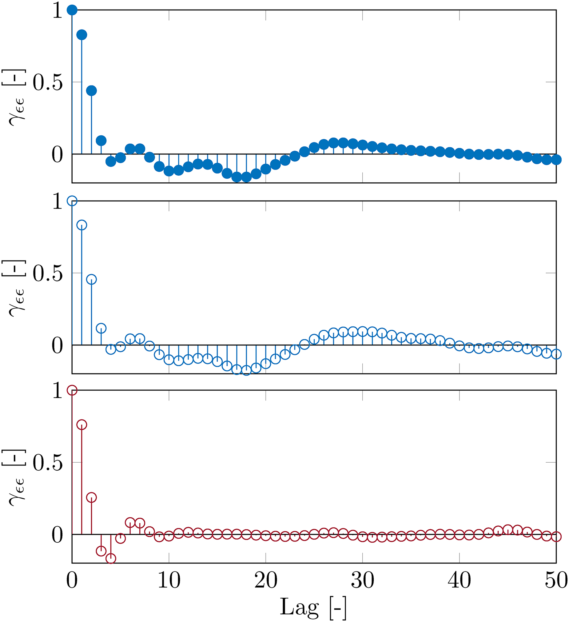
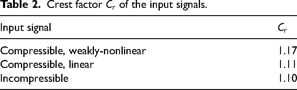
The amplitude of the broadband excitation signal is scaled from $f_{\mathrm{ex}}/{\overline{u}}_{\mathrm{ex}}=0.1$ to $f_{\mathrm{ex}}/{\overline{u}}_{\mathrm{ex}}=0.065$ . This downscaling results in the same broadband signal for compressible and incompressible simulation, but different amplitudes. The PDF of the down-scaled excitation signal is shown in Figure 10 (left column). The corresponding input signal (right column) of the compressible LES now leads to a similar PDF as in the incompressible case with maximum amplitudes $u_{\mathrm{ref}}^{\mathrm{\prime }}/{\overline{u}}_{\mathrm{ref}}\approx 0.1$ . The peak in the frequency domain (middle column) also decreases in amplitude, but persists because the resonance in the compressible LES does not disappear. Note that there is no peak in the PSD of the incompressible signal, which is beneficial for the quality of the signal. The difference in PDF of the input signals can be quantified with the crest factor (see equation (8)) of the input signals of weakly-nonlinear compressible, compressible, and incompressible LES, as shown in Table 2. The compressible and incompressible input signals have a similar $C_{\mathrm{r}}$ and therefore show a better utilization of the signal power compared to the weakly-nonlinear compressible LES, which has a higher crest factor. Finally, the autocorrelation $\gamma$ of the input signals is evaluated according to equation (9) and shown in Figure 12. The signals of the two compressible simulations have a similar autocorrelation behavior, where both exhibit correlation with itself up to around 40 time lags. The autocorrelation of the incompressible LES decays to zero within 10 time lags. Thus, the resonances in the compressible simulations significantly increase (i.e. degrade) the autocorrelation. Overall, the incompressible signal has the highest signal quality. The input signal of the compressible LES shows the same crest factor as the incompressible signal and comparable amplitudes in the PSD, only the autocorrelations differ significantly. The input signal of the weakly nonlinear compressible LES shows the poorest quality in all three aspects compared to the two linear signals.

Figure 12.

Autocorrelation $\gamma$ of the weakly-nonlinear compressible (top), compressible (middle) and incompressible (bottom) input signals.

Table 2.

Crest factor $C_{\mathrm{r}}$ of the input signals.

Input signal	$C_{\mathrm{r}}$
Compressible, weakly-nonlinear	1.17
Compressible, linear	1.11
Incompressible	1.10

With the evaluation of the input and output signals, the following becomes clearer:

The quality of the excitation signal in the incompressible simulation can be directly tuned/adjusted due to the absence of acoustic wave propagation. The input signal is equivalent to the excitation signal in the incompressible case, which leads to the conclusion that the power spectra are also equivalent (not shown in Figure 10).

The input signal and excitation signal may differ significantly from each other in a compressible LES, as a result of acoustic resonances in the system (see equation (3)). The more dominant the outgoing acoustic wave $g$ —which can occur in an anechoic system with ITA resonances—the larger the difference between the incoming acoustic wave $f$ and the velocity perturbations $u^{\mathrm{\prime }}$ . With increased (acoustic or ITA) resonances in a compressible LES, the quality of the excitation signal is deteriorated, which may affect the accuracy of system identification.

The PDF support of the input signal, which quantifies the occurrence of amplitudes in the time series, can be seen as a first indicator of nonlinear flame behavior.

Identification of flame response from compressible and incompressible LES

The main objective of the present work is to ascertain if compressible and incompressible CFD/SI predicts the same flame response. For this reason, the FTF is identified from both data sets and then compared with experimental measurements.

Uncertainty in system identification promoted by turbulent combustion may be important if broadband forcing is performed. Note that the spectral distribution of combustion noise is detrimental for system identification, as the input signals may exhibit low SNR per frequency. Therefore, as a first step, harmonic forcing of compressible and incompressible LES at specific frequencies 140 Hz, 180 Hz and 360 Hz is investigated. The excitation amplitude of the compressible LES is chosen such that the amplitude at the reference position (i.e. of the input signal) equals $u_{\mathrm{ref}}^{\mathrm{\prime }}/{\overline{u}}_{\mathrm{ref}}=0.1$ . Gain and phase of time series data is analyzed using a fast Fourier transform (FFT) based approach. The harmonic time-series data ( $\approx 300$  ms) is split into parts of eight consecutive periods, where each part overlaps with seven periods from the previous part. This procedure is used to compute the standard deviation from a large data set, which is necessary because of the noise introduced by turbulent combustion. The harmonic results with respective standard deviation of $1.96$ $\sigma$ ( $95\text{\%}$ confidence interval) are shown in Figure 13. Both, the magnitude and phase of the compressible and incompressible LES at each of the frequencies under investigation agree very well.

After harmonic analysis, the LES is excited with a broadband signal to obtain a FTF up to $500$  Hz. The finite impulse response (FIR) identification is applied to a $500$  ms time series generated by compressible and incompressible LES, where the first $30$  ms are cut as a transient phase. A polynomial order $n_h=39$ is considered for both simulations. The FTFs with $1.96$ $\sigma$ confidence intervals ⁷⁰ from compressible and incompressible CFD/SI are compared with experimental measurements in Figure 13. The gain of the transfer functions from CFD/SI stands in overall good agreement with each other and with experimental values. It approaches unity in the low frequency limit ⁷¹ and features the overall low-pass behavior with excess in gain at $90$  Hz followed by a local minimum at $220$  Hz^72,73. At $200$  Hz both CFD/SI results have a slightly smaller gain than in experiment. This mismatch might be caused by the sensitivity of the sum (see equation (7)) to uncertainties in $h_k$ when the sum approaches zero (cancellation effects in the Nyquist plot as discussed in more detail by Polifke ⁴² ).

The small disagreement between the FTFs of compressible and incompressible CFD/SI may have different origins. A likely reason is the inherent stochasticity of the system under evaluation: a turbulent flame. Such a stochastic system introduces uncertainties in the flame response estimation. Note, however, that differences in the prediction lie in the confidence interval of the respective counterpart. Both methodologies show the typical characteristic features of a premixed FTF ⁴² , as discussed in detail above. Both results resolve the first and second maximum of the FTF gain very well. Furthermore, the phase, which is essential for an accurate thermoacoustic analysis ¹ , matches very well the experimental data. It decreases nearly monotonically with a slight deviation around $250$ Hz, which is close to the local minimum in gain.

To further analyze the system dynamics, the $-\pi$ criterion can be used to characterize the ITA modes in the anechoic environment^30,37,32. The frequencies with a phase corresponding to an odd multiple of $-\pi$ are evaluated. The ITA frequencies extracted from compressible CFD/SI ( $f_{\mathrm{ITA}1}=109.5$  Hz and $f_{\mathrm{ITA}2}=250.8$  Hz) and incompressible CFD/SI ( $f_{\mathrm{ITA}1}=109.7$  Hz and $f_{\mathrm{ITA}2}=262.4$  Hz) match very well. These frequencies correspond to the peaks observed in the PSD of the compressible simulations in Figure 10 (middle column). The overall good agreement in FTF gain and phase will lead to similar thermoacoustic stability predictions, which can be analyzed in detail by incorporating the FTFs into a reduced order network model of the burner (not done in the present work).

Conclusion

In the present work, the FTF of an acoustically compact premixed burner was identified. In this context, compressible simulation is often the choice for generating the required time series. However, as shown by many authors^14,17–21, incompressible simulation is a well suited alternative. We demonstrated for the first time that both methodologies predict the same flame response to upstream velocity perturbations, reproduce the experimental results equally well, and show the characteristic features of the FTF in fully premixed combustion. For a direct comparison of the flame dynamics in both methods, the same computational setup (i.e. grid, numerical schemes, turbulent combustion model, chemistry mechanism) was used in the present study to exclude systematic errors. One might conclude that both compressible and incompressible CFD are valid methods for analyzing the dynamics of acoustically compact velocity sensitive flames, provided that an excitation level is assured that results in linear flame response and aleatoric uncertainty from the stochastic nature of the identification method is considered. However, the current work reveals significant challenges in compressible simulation for FTF identification.

The present study demonstrated explicitly that there is no need of including acoustic wave propagation in the CFD formulation, since flame-acoustics interaction, for an acoustically compact premixed flame, has no influence on the latter. Excluding the acoustics from the governing equations allows the incompressible simulation to circumvents acoustic resonances and feedback loops in the system. This is equivalent to a perfectly thermoacoustically stable system without any resonances. Besides, statistically steady-state flow and flame quantities (i.e. velocity temperature, heat release rate) were shown to be equivalent.

In the compressible simulation, on the other hand, depending on the reflection coefficients (non-reflecting, fully reflecting, partially reflecting) the amplitude of thermoacoustic modes—either of ITA or acoustic origin—can be amplified by resonances ³⁸ , which increases the SNR and therefore corrupts the subsequent identification procedure. Due to acoustic wave propagation, sophisticated acoustic boundary conditions^40,28,29 are required in compressible simulation to obtain a thermoacoustically stable system. Note that even these systems exhibit acoustic modes, which are manifested as peaks in the power spectrum. A key message of this work is that a forcing signal with small amplitudes does not guarantee an input signal (upstream velocity perturbation) with small amplitudes (i.e. linear flame response) and similar signal quality, which is detrimental for the identification of the linear flame response with high confidence and accuracy. It is emphasized that the choice of the excitation amplitude in compressible LES is not trivial and may need iterative adjustment until linear response is obtained.

Implicit pressure-based solvers are used in the present work, where there is no acoustic CFL number constraint besides numerical stability limitations and accuracy. Nevertheless, the computational effort is by a factor 3 higher in our compressible simulations. The extent to which incompressible simulations are computationally more efficient depends highly on the underlying numerics ²² and is not object of the present work.

In conclusion, we recommend the incompressible CFD/SI approach for studies on flame response identification in acoustically compact, premixed flames due to the above-mentioned difficulties for the compressible counterpart. While LES was used in the present work, the outcome generalizes to other CFD methods like RANS or direct numerical simulation (DNS). It should be further noted that not all signal quality criteria are of the same significance for the identification of flame dynamics. In the present study, for example, an identical FTF up to the confidence interval is obtained with compressible and incompressible input signals, even though they exhibit a different degree of autocorrelation. The impact of individual quality features like crest factor, power spectrum, and autocorrelation of the input signal on the system identification of premixed flames needs further investigation. In addition, the study should be extended to non-compact flames, since acoustic compactness cannot be assumed in many applied combustors.