Sage Journals: Discover world-class research

Abstract

Background:

Epilepsy is a chronic neurological disorder characterized by recurrent seizures that significantly impact patients’ quality of life. Identifying predictors is crucial for early intervention.

Objective:

Electroencephalography (EEG) microstates effectively describe the resting state activity of the human brain using multichannel EEG. This study aims to develop a comprehensive prediction model that integrates clinical features with EEG microstates to predict drug-refractory epilepsy (DRE).

Design:

Retrospective study.

Methods:

This study encompassed 226 patients with epilepsy treated at the epilepsy center of a tertiary hospital between October 2020 and May 2023. Patients were categorized into DRE and non-DRE groups. All patients were randomly divided into training and testing sets. Lasso regression combined with Stepglm [both] algorithms was used to screen independent risk factors for DRE. These risk factors were used to construct models to predict the DRE. Three models were constructed: a clinical feature model, an EEG microstate model, and a comprehensive prediction model (combining clinical-EEG microstates). A series of evaluation methods was used to validate the accuracy and reliability of the prediction models. Finally, these models were visualized for display.

Results:

In the training and testing sets, the comprehensive prediction model achieved the highest area under the curve values, registering 0.99 and 0.969, respectively. It was significantly superior to other models in terms of the C-index, with scores of 0.990 and 0.969, respectively. Additionally, the model recorded the lowest Brier scores of 0.034 and 0.071, respectively, and the calibration curve demonstrated good consistency between the predicted probabilities and observed outcomes. Decision curve analysis revealed that the model provided significant clinical net benefit across the threshold range, underscoring its strong clinical applicability. We visualized the comprehensive prediction model by developing a nomogram and established a user-friendly website to enable easy application of this model (https://fydxh.shinyapps.io/CE_model_of_DRE/).

Conclusion:

A comprehensive prediction model for DRE was developed, showing excellent discrimination and calibration in both the training and testing sets. This model provided an intuitive approach for assessing the risk of developing DRE in patients with epilepsy.

Keywords

drug-refractory epilepsy electroencephalography microstates Lasso nomogram prediction model Stepglm

Introduction

Epilepsy is a chronic neurological disorder characterized by recurrent episodes of abnormal and excessive electrical discharge in the brain, leading to transient central nervous system dysfunction.¹ Unfortunately, around 30% of these patients do not respond to conventional antiseizure medication (ASM) and develop drug-refractory epilepsy (DRE).¹ Prolonged or frequent seizures, as well as status epilepticus, can severely impact patients’ cognition, memory, quality of life, and psychological well-being.¹ The International League Against Epilepsy (ILAE) defines DRE as the failure of two well-tolerated and appropriately selected antiseizure medication regimens, used alone or in combination, to achieve sustained seizure freedom.² Consequently, early diagnosis of DRE is crucial to improve patient outcomes.³

The development of DRE is associated with various factors, including specific types of epilepsy syndromes, age of onset, multiple seizure types, clear neuroimaging abnormalities such as hippocampal sclerosis, cortical dysplasia, tumors, and traumatic lesions, widespread epileptiform electroencephalography (EEG) changes, and previous treatment failure with ASMs.^4,5 Several prediction models and predictors have been proposed to improve clinical outcomes for patients with DRE. However, the currently available indicators for guiding clinical practice are still limited due to their lack of specificity and sensitivity, limited generalizability, and high cost.

EEG is the most important tool for diagnosing and distinguishing epilepsy. Research has shown that spontaneous brain activity during resting state accounts for 80% of total brain energy.⁶ Resting-state EEG analysis involves various methods such as power spectrum analysis,⁷ whole-brain domain synchronization,⁸ functional network connectivity,⁹ and EEG microstates.¹⁰ EEG microstates are an effective method for describing the resting state activity of the human brain using multichannel EEG.¹⁰ The concept of EEG microstates originated from the observation that broad-band spontaneous EEG activity during rest can be characterized by a finite set of scalp potential topographies.¹⁰ These configurations remain quasi-stable for a distinct duration before swiftly transitioning into a new topographical arrangement.¹¹ These periods of quasi-stability, reflecting the pace at which humans process information, are known as microstates.¹² These microstates signal the “near-simultaneous activity among nodes within large-scale networks.”¹² Each microstate typically lasting 60–120 ms.¹³ About 70% of EEG signals can be adequately represented by four microstates, labeled as A, B, C, and D.^8,14 Microstate A connects to brain activity in the temporal cortex and left insula, suggesting a function in language processing.^15,16 Microstate B, linked to the occipital region, is involved in visual processing.^15,16 EEG activity in the cingulate gyrus, inferior frontal gyrus, insula, and precuneus gyrus associates with microstate C, which participates in subjective perception and autonomic processing.¹⁵ Microstate D is thought to be involved in attention and analytical processing and has been shown to be linked to neural activity in the right hemispheric regions of the frontal and parietal cortices.¹⁵

EEG microstate measures, including average duration, coverage, frequency, and transition probability (TP), describe changes in brain states and reflect abnormalities in brain network function.^10,17 EEG microstate analysis has been extensively applied in the field of neuropsychiatric disorders, including schizophrenia,¹⁸ dementia,¹⁹ and narcolepsy.²⁰ These findings suggest that EEG microstate analysis could serve as an effective tool for identifying abnormalities associated with brain disorders.^19,20 Although EEG microstate is commonly employed to examine brain function, its application in studying DRE through EEG microstate analysis has been relatively underexplored. Functional connections between subcortical and cortical structures undergo alterations during epileptic seizures. These changes imply shifts in patterns of brain activity, which may offer valuable insights into microstate variations after seizures.²¹

While various predictive models for DRE exist,²² none currently combines clinical features with EEG microstates. This study aimed to develop a nomogram model by integrating clinical features with EEG microstates, and to assess the model’s performance in predicting DRE. This approach aims to offer novel reference indicators for the diagnosis of DRE.

Materials and methods

Participants and data acquisition

Participants

We retrospectively investigated a total of 226 patients with epilepsy who were treated between October 2020 and May 2023 at the epilepsy center of Fujian Medical University Union Hospital. The inclusion criteria were as follows: (1) Patients who met the ILAE’s definition of epilepsy²; (2) patients who underwent video electroencephalography (VEEG) monitoring; (3) patients with a complete medical history, neurological examination, and magnetic resonance imaging (MRI) data; and (4) patients who regularly took ASMs. The ASMs administered to patients in this study included sodium valproate, oxcarbazepine, carbamazepine, levetiracetam, lamotrigine, perampanel, topiramate, phenytoin, phenobarbital, and clonazepam. The exclusion criteria were as follows: (1) patients lacking VEEG monitoring; (2) patients with incomplete medical records; (3) patients suffering from severe liver or kidney disease; and (4) patient with irregular ASMs therapy and poor compliance.

The patients were categorized into two groups based on their follow-up records, as shown in Figure 1. Participants were enrolled in the non-DRE (NDRE) group (n = 77) if they achieved freedom from all types of seizures for 12 months or three times the pre-intervention interseizure interval, whichever was longer, after receiving appropriate ASM therapy.² Participants were enrolled in the DRE group (n = 149) after failing to achieve sustained seizure freedom despite adequate trials of two ASM regimens, which were both tolerated and appropriately chosen and used, whether as monotherapies or in combination.²

Figure 1.

Flow chart.

Clinical features

This study includes the following clinical feature variables: continuous variables and categorical variables. Continuous variables included: age, body mass index (BMI), educational years, age at onset, and duration of epilepsy. Categorical variables included: (1) gender; (2) educational level (primary, senior, college, or above); (3) family history of epilepsy; (4) type of epilepsy (focal, generalized, focal secondary generalized, multiple, and unknown onset); and (5) initial seizure frequency. Initial seizure frequency is referred to as the frequency of patients’ experience before starting treatment with ASMs, categorized as follows: (1) Daily: the patient experienced seizures every day. (2) Weekly: the patient experienced at least one seizure every week. (3) Monthly: the patient experienced at least one seizure every month. (4) Yearly : the patient experienced seizures at intervals longer than a month, not fitting into the daily, weekly, or monthly categories. (5) Etiology (genetic, structural, immunological, metabolic, infectious, and unknown). (6) History of status epilepticus. (7) History of generalized tonic-clonic seizures (GTCS). (8) Nocturnal seizures. (9) History of febrile seizures. (10) EEG findings: results of an EEG examination, categorized as normal EEG (1), EEG with abnormal background (2), and EEG with epileptiform discharge (3). (11) MRI findings: MRI positivity indicates radiological abnormalities related to epilepsy, the epilepsy-related radiological abnormalities primarily included the following: brain tumors, stroke lesions, vascular malformations, hippocampal sclerosis, cortical dysplasia, post-traumatic lesions, central nervous system infection. (12) Absence epilepsy. (13) Comorbid cognitive disorder. The Montreal Cognitive Assessment (MoCA) and Mini-Mental State Examination (MMSE) were used to assess cognition. MMSE ⩽ 19 for illiterates, ⩽22 for those with elementary school education, and ⩽26 for those with junior high school education and above. According to the Chinese MoCA criteria, illiterates ⩽13, those with 1–6 years of education ⩽19, and those with 7 or more years of education ⩽24.²³ (14) Comorbid Psychiatric disorder. (15) Comorbid depression. The Self-rating Depression Scale (SDS) was employed to evaluate depression. SDS index scores of 25–49 (raw score 20–40) were normal; SDS index scores of 50 or more (raw score = 40) indicated the presence of depressive symptoms.²⁴

EEG acquisition and preprocessing

Resting-state EEG acquisition

Subjects washed their hair prior to EEG collection, refrained from using oily cleaning or hair care products, recorded their scalp EEG in a quiet and relaxed state. All patients with epilepsy underwent VEEG recording. To avoid slow waves caused by hunger, patients were required to have normal meals during the monitoring period. EEG data were recorded continuously for 24 h, and a 10-min segment of EEG data during which the patients were awake was extracted for analysis.

VEEG recordings were performed using an EEG recorder (EEG-1200C, Japan) with 19 scalp electrodes and two reference electrodes placed strictly according to the international 10 20 system. Video and EEG data were recorded in a synchronized manner. Electrodes (Fp1, Fp2, F3, F4, F7, F8, T7, T8, P7, P8, C3, C4, P3, P4, O1, O2, Fz, Cz, and Pz) were positioned precisely using a standardized ruler.²¹ The electrical impedance of the scalp electrodes was less than 5 kΩ. The EEG-1200C had a sampling rate of 500 Hz, the low-pass filter rate was 70 Hz, and the high-pass filter rate was 0.5 Hz. Epileptic seizures and epileptiform discharges were analyzed and marked by two experienced EEG technicians.

EEG data preprocessing

The preprocessing of EEG data was carried out using Matlab R2013b software (MathWorks, Inc., Natick, MA, USA) equipped with the EEGLAB toolbox.²⁵ The steps involved in preprocessing are as follows: (1) Importing raw data: the raw EEG data were first imported into the EEGLAB toolbox. (2) Electrode localization: we localized the electrodes according to the standard 10–20 system. (3) Interpolating bad electrodes: any electrodes with poor signal quality were interpolated to ensure data consistency. (4) Removing time segments with excessive drift: time segments with excessive drift or noise were identified and removed to enhance data quality. (5) Downsampling: the continuous EEG data were downsampled to 250 Hz to reduce computational load while retaining essential signal information. (6) Segmentation into epochs: the downsampled EEG data were segmented into 2-s epochs to facilitate analysis. (7) Band-pass filtering: a band-pass filter was set from 1 to 40 Hz to focus on the frequency range of interest, which includes most of the relevant brain wave frequencies. (8) Notch filtering: a notch filter was applied at 50 Hz to eliminate line noise commonly found in EEG recordings. (9) Artifact removal using independent component analysis (ICA): ICA was employed to effectively remove artifacts caused by eye movements, heartbeats, and muscle activity, thereby improving the signal quality for subsequent analysis. (10) Readjusting the filter: finally, the filter was readjusted to 2–20 Hz to further refine the signal for the microstate analysis. For each patient, we retained 3 min of EEG data, which correspond to a total of 90 epochs.²⁶

EEG microstate analysis

EEG microstate analysis was performed using Cartool software following EEG data preprocessing,²⁷ adhering to a standardized procedure from previous studies.^28,29 The analysis involved three principal steps: First, we computed the global field power (GFP) to assess potential variations across electrodes at specific time points.¹⁴ When GFP reaches its peak, the EEG topography is deemed stable, and these topographies are defined as microstates.¹⁴ Subsequently, clustering analysis was applied to the GFP’s local maxima.^14,28 The topographical maps at these GFP peaks were recognized as unique microstates, illustrating the dynamic shifts in EEG signals as transitions occur between these states.²⁷ Utilizing a modified version of the K-means clustering algorithm,³⁰ we identified four distinct microstate topographies: A, B, C, and D. Finally, we calculated four parameters for each microstate—duration, frequency, coverage, and TPs¹⁴—to collectively depict variations in the brain’s states.

Duration referred to the average length of time (in milliseconds) during which a given EEG microstate remains stable/present, reflecting the stability of neural activity in the cerebral cortex.¹⁴ Frequency represented the number of times an EEG microstate repeats within 1 s (in occurrences per second), indicative of the frequency or tendency of activation in the underlying neural populations or systems.¹⁴ Coverage represented the percentage of total time covered by a specific EEG microstate category (in percentages).¹⁴ TPs indicated the probabilities of transitions between different EEG microstates (in percentages).¹⁴

Modeling process

After completing the above steps, we used the “createDataPartition” function from the “caret” package to split the dataset into training and testing sets in a 0.5:0.5 ratio. We randomly selected 50% of the NDRE group (39 cases) and 50% of the DRE group (75 cases) to form the training set, totaling 114 samples. The remaining 50% of the dataset, consisting of 38 NDRE patients and 74 DRE patients, comprised the test set, totaling 112 samples.

To establish and validate a comprehensive model for predicting DRE, we employed multiple machine learning algorithms. Initially, we integrated 10 algorithms: Lasso, Ridge, Elastic Net (Enet), Stepwise GLM (Stepglm), support vector machine (SVM), glmBoost, linear discriminant analysis (LDA), random forest (RF), gradient boosting machine (GBM), and naïve Bayes.³¹ We then created 48 combinations of these algorithms. In each combination, the first algorithm was used for important variable selection, and the second algorithm was further used for refinement and modeling. The important variables identified varied across different algorithm combinations (Supplemental Table).

To reduce random errors in data partitioning, prevent information leakage, and ensure algorithm stability, we used a 10-fold cross-validation method.³² Utilizing the “createMultiFolds” function from the “caret” package, we performed 10-fold cross validation repeated 200 times. The dataset was randomly divided into 10 subsets (“folds”), with 9 subsets used for training and 1 subset used for testing. This process was repeated 10 times, with each subset used as the test set once.³² By averaging the performance metrics across all folds, we ensured that the model’s evaluation is robust and not dependent on a specific data split, ultimately aiding in the selection of the most optimal model.

The initial training of the models was conducted on the training set, followed by testing the model performance on the test set. Each model’s performance was assessed by calculating Harrell’s concordance index (C-index), and the model with the highest average C-index was selected as the optimal model. In this study, three predictive models for DRE were constructed: (1) a clinical model, consisting solely of clinical features; (2) an EEG model, based solely on EEG microstate feature parameters; and (3) a CE model, combining clinical features with EEG microstate analysis feature parameters.

To compare the performance of the three predictive models with other models, we retrieved published models by searching PubMed for articles published. We used the following Boolean terms for our search: (“epilepsy” OR “seizure” OR “convulsion”) AND (“refractory” OR “drug-resistant” OR “pharmacoresistant” OR “intractable” OR “drug response” OR “prognosis”) AND (“risk factor” OR “predictor” OR “predictive”). We then selected original publications that established models relevant as comparisons to the three DRE predictive models.^33–60

Model performance evaluation

For each model, the concordance index (C-index) or area under the curve (AUC) was calculated across all datasets, and the model boasting the highest average C-index or AUC was deemed the optimal model. These results were then benchmarked against multiple existing prediction models. To assess the agreement between the model’s predicted outcomes and actual results, a calibration curve was plotted. Decision curve analysis (DCA) was performed to evaluate the utility of these models. Additionally, a nomogram and a website were developed to visualize the model’s structure.

Statistical analysis

All data processing, statistical analysis, and graphing were conducted using R software version 4.2.2. (R Foundation for Statistical Computing, https://www.r-project.org) Continuous variables were presented as mean ± standard deviation and categorical variables were presented as n (%). Continuous variables were tested using Student’s t-test or one-way ANOVA, as appropriate. Categorical variables were tested using the Chi-square test or Fisher’s exact test, as appropriate. Feature correlations were calculated using the Pearson correlation coefficient, with visualization performed using heatmaps. The “createDataPartition” function from the “caret” package was used to split the dataset into training and testing sets in a 0.5:0.5 ratio. The Receiver Operating Characteristic (ROC curve for predicting binary classification variables was implemented using the “pROC” package in R software. Figures were drawn using the “ggplot2” and “Regplot” packages. The “shiny” package is employed to create a web calculator, providing users with an interactive data analysis tool. The false discovery rate (FDR) was employed for multiple test correction. A p-value of <0.05 was considered statistically significant.

Results

Patients characteristics

A total of 226 patients were included in the study, including 110 males and 116 females, with an average age of 32.465 ± 14.166 years. The NDRE group consisted of 77 patients, including 39 males (50.65%) and 38 females (49.35%), with an average age of 32.234 ± 16.351 years. The DRE group consisted of 149 patients, including 71 males (47.65%) and 78 females (52.35%), with an average age of 32.584 ± 12.952 years.

Description of clinical features and analysis of EEG microstate features

The results showed no significant differences between the NDRE and DRE groups in terms of gender, age, BMI, educational level and years, family history of epilepsy, type of epilepsy, etiology of epilepsy, history of status epilepticus, history of GTCS, nocturnal seizures, history of febrile seizures, MRI findings, comorbid cognitive disorders, and comorbid psychiatric disorders (all p > 0.05). However, significant differences were observed in the duration of epilepsy, age at onset, initial seizure frequency, abnormal EEG findings, absence epilepsy, and comorbid depression between the two groups (all p < 0.01), as demonstrated in Table 1 and Figure 2. After applying the FDR for multiple testing correction, statistically significant differences in the duration of epilepsy, initial seizure frequency, EEG findings, absence epilepsy, and comorbid depression between the two groups were still evident.

Table 1.

Baseline epilepsy patient characteristics in the DRE and NDRE groups.

Characteristic	Level	Overall	NDRE	DRE	p-Adjust
n		226	77	149
Gender (%)	Female	116 (51.33)	38 (49.35)	78 (52.35)	0.7741
	Male	110 (48.67)	39 (50.65)	71 (47.65)
Age (years)		32.465 (14.166)	32.234 (16.351)	32.584 (12.952)	0.9021
BMI (kg/m²)		21.870 (3.435)	21.562 (3.045)	22.029 (3.619)	0.3435
Educational level (%)	Primary	40 (17.70)	12 (15.58)	28 (18.79)	0.7478
	Senior	113 (50.00)	38 (49.35)	75 (50.34)
	College or above	73 (32.30)	27 (35.06)	46 (30.87)
Educational years		10.606 (3.629)	11.143 (3.772)	10.329 (3.534)	0.1488
Family history of epilepsy (%)	No	16 (7.08)	3 (3.90)	13 (8.72)	0.2856
	Yes	210 (92.92)	74 (96.10)	136 (91.28)
Duration of epilepsy (years)		11.641 (9.792)	7.414 (7.433)	13.825 (10.164)	<0.0001
Age at onset (years)		20.537 (14.912)	24.279 (16.630)	18.603 (13.600)	0.0158
Type of epilepsy (%)	Focal	67 (29.65)	19 (24.68)	48 (32.21)	0.6836
	Generalized	18 (7.96)	6 (7.79)	12 (8.05)
	F_to_G	29 (12.83)	11 (14.29)	18 (12.08)
	Multiple	47 (20.80)	15 (19.48)	32 (21.48)
	unknown	65 (28.76)	26 (33.77)	39 (26.17)
Initial seizure frequency (%)	Daily	23 (10.18)	0 (0.00)	23 (15.44)	<0.0001
	Weekly	14 (6.19)	0 (0.00)	14 (9.40)
	Monthly	55 (24.34)	4 (5.19)	51 (34.23)
	Yearly	134 (59.29)	73 (94.81)	61 (40.94)
Etiology (%)	Genetic	6 (2.65)	1 (1.30)	5 (3.36)	0.2735
	Structural	65 (28.76)	21 (27.27)	44 (29.53)
	Infectious	4 (1.77)	3 (3.90)	1 (0.67)
	unknown	151 (66.81)	52 (67.53)	99 (66.44)
History of SE (%)	No	186 (82.30)	63 (81.82)	123 (82.55)	1
	Yes	40 (17.70)	14 (18.18)	26 (17.45)
History of GTCS (%)	No	59 (26.11)	20 (25.97)	39 (26.17)	1
	Yes	167 (73.89)	57 (74.03)	110 (73.83)
Nocturnal seizure (%)	No	80 (35.40)	25 (32.47)	55 (36.91)	0.6062
	Yes	146 (64.60)	52 (67.53)	94 (63.09)
History of febrile seizure (%)	No	189 (83.63)	66 (85.71)	123 (82.55)	0.6748
	Yes	37 (16.37)	11 (14.29)	26 (17.45)
EEG findings (%)	Normal	27 (11.95)	18 (23.38)	9 (6.04)	0.0007
	Abnormal background	4 (1.77)	1 (1.30)	3 (2.01)
	Epileptiform discharges	195 (86.28)	58 (75.32)	137 (91.95)
MRI findings (%)	Negative	157 (69.47)	57 (74.03)	100 (67.11)	0.3592
	Positive	69 (30.53)	20 (25.97)	49 (32.89)
Absence epilepsy (%)	No	191 (84.51)	73 (94.81)	118 (79.19)	0.004
	Yes	35 (15.49)	4 (5.19)	31 (20.81)
Comorbid cognitive disorder (%)	No	38 (16.81)	8 (10.39)	30 (20.13)	0.0952
	Yes	188 (83.19)	69 (89.61)	119 (79.87)
Comorbid psychiatric disorders (%)	No	8 (3.54)	1 (1.30)	7 (4.70)	0.3519
	Yes	218 (96.46)	76 (98.70)	142 (95.30)
Comorbid depression (%)	No	72 (31.86)	15 (19.48)	57 (38.26)	0.0065
	Yes	154 (68.14)	62 (80.52)	92 (61.74)

DRE, drug-refractory epilepsy; EEG, electroencephalography; GTCS, generalized tonic-clonic seizures; MRI: magnetic resonance imaging; n, number of patients; NDRE, non-drug-refractory epilepsy group; SE, status epilepticus.

Figure 2.

Clinical features. Compare the age at onset, duration of epilepsy, initial seizure frequency, EEG findings, absence epilepsy, and comorbid depression between the two groups: (a) correspond to the age at onset, (b) correspond to the duration of epilepsy, (c) correspond to the initial seizure frequency, (d) correspond to the EEG findings, (e) correspond to the absence epilepsy, and (f) correspond to comorbid depression.

The microstate maps were classified into four distinct categories as A, B, C, and D. Supplemental Figure visually presents the microstate topographic classes observed within the DRE group and NDRE group.

For microstates B and D, the differences in duration, frequency, and coverage between the two groups were statistically significant. The average duration, frequency, and coverage of microstate B in the DRE group were higher than those in the NDRE group. Conversely, the three indicators for microstate D were lower in the DRE group compared to the NDRE group. The duration of microstate C was statistically significantly shorter in the DRE group than in the NDRE group. For microstate A, the differences in duration, frequency, and coverage between the two groups were not statistically significant (all p > 0.05). The TPs between the two groups were statistically significant (all p < 0.001), as demonstrated in Table 2 and Figure 3. After applying the FDR for multiple testing correction, these differences were still found to be statistically significant.

Table 2.

Comparison of EEG microstate features between NDRE and DRE groups.

Variables	Level	Overall	NDRE	DRE	p-Adjust
Microstate A	Duration	114.536 (12.916)	114.440 (12.456)	114.586 (13.189)	0.9358
	Coverage	28.391 (6.960)	28.807 (6.855)	28.176 (7.027)	0.5553
	Frequency	3.982 (0.617)	4.054 (0.661)	3.944 (0.592)	0.2564
Microstate B	Duration	104.034 (10.649)	96.671 (9.800)	107.839 (8.962)	<0.0001
	Coverage	23.557 (5.831)	18.170 (4.792)	26.341 (4.122)	<0.0001
	Frequency	3.702 (0.696)	3.109 (0.586)	4.008 (0.532)	<0.0001
Microstate C	Duration	101.333 (11.400)	103.460 (10.185)	100.234 (11.864)	0.0476
	Coverage	21.442 (5.390)	22.335 (5.166)	20.981 (5.462)	0.0910
	Frequency	3.481 (0.540)	3.553 (0.487)	3.443 (0.563)	0.1547
Microstate D	Duration	110.103 (15.440)	117.878 (17.627)	106.086 (12.457)	<0.0001
	Coverage	26.610 (5.909)	30.689 (5.497)	24.502 (4.943)	<0.0001
	Frequency	3.925 (0.535)	4.216 (0.485)	3.775 (0.497)	<0.0001
TP of microstates	A → B	0.090 (0.027)	0.071 (0.015)	0.099 (0.026)	<0.0001
	A → C	0.080 (0.015)	0.084 (0.016)	0.077 (0.014)	0.0013
	A → D	0.094 (0.026)	0.115 (0.027)	0.084 (0.017)	<0.0001
	B → A	0.089 (0.026)	0.070 (0.014)	0.098 (0.026)	<0.0001
	B → C	0.071 (0.016)	0.062 (0.013)	0.075 (0.016)	<0.0001
	B → D	0.085 (0.018)	0.076 (0.018)	0.090 (0.016)	<0.0001
	C → A	0.080 (0.015)	0.086 (0.017)	0.077 (0.013)	<0.0001
	C → B	0.070 (0.017)	0.060 (0.014)	0.075 (0.016)	<0.0001
	C → D	0.081 (0.023)	0.092 (0.020)	0.075 (0.022)	<0.0001
	D → A	0.095 (0.025)	0.114 (0.026)	0.084 (0.018)	<0.0001
	D → B	0.085 (0.017)	0.077 (0.017)	0.090 (0.016)	<0.0001
	D → C	0.081 (0.023)	0.092 (0.019)	0.075 (0.023)	<0.0001

A, Microstate A; B, Microstate B; C, Microstate C; D, Microstate D; DRE, drug-refractory epilepsy; n, number of patients; NDRE, non-drug-refractory epilepsy group; TP, transition probabilities; →, transition probability from one microstate to another microstate.

Figure 3.

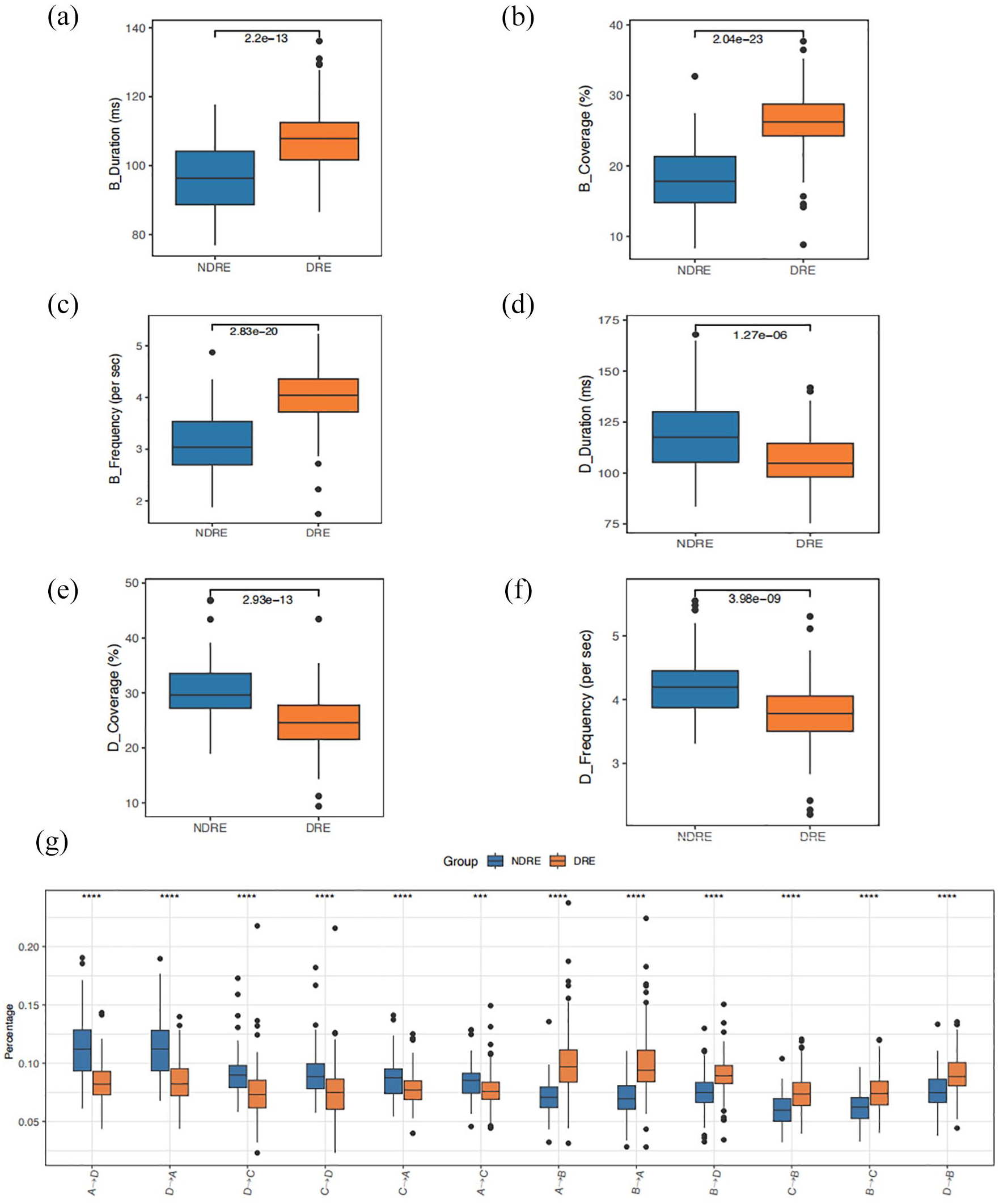
EEG microstate features. Compare the duration, frequency, coverage of each microstate, and transition probabilities between each microstate between the two groups: (a) correspond to the duration of microstate B, (b) correspond to the coverage of microstate B, (c) correspond to the frequency of microstate B, (d) correspond to the duration of microstate D, (e) correspond to the coverage of microstate D, (f) correspond to the frequency of microstate D, and (g) transition probabilities between each microstate.

To investigate the correlations among feature variables, we calculated the correlation coefficients between two groups of distinct variables and visualized the results. The results are presented in Supplemental Figures 1 and 2.

Model establishment

We integrated 10 machine learning algorithms and 48 algorithm combinations. The AUC was computed for each algorithm. Select the algorithm with the highest average AUC as the optimal algorithm. The evaluation results of the algorithms were then visually presented using a heatmap (Figure 4(a)). Interestingly, the optimal algorithm was a combination of Lasso and Stepglm (direction = both) with the highest average AUC (0.98) (Figure 4(a)).

Figure 4.

A prediction algorithm was developed and validated via the machine learning-based integrative procedure. Establish three models and compare them with other models: (a) a total of 10 machine learning algorithms and 48 algorithm combinations. The integrative algorithms included Lasso, Ridge, Enet, Stepglm, SVM, glmBoost, LDA, RF, GBM, and naïve Bayes. Further calculated the AUC of each model across all datasets, (b) the optimal lambda was obtained when the partial likelihood deviance reached the minimum value, and plot a vertical dashed line at the optimal value. The optimal lambda value yielded 10 non-zero coefficients, (c) coefficients of eight variables were finally obtained in the Stepglm [both] model, (d) C-index analysis of three models and 28 published other models in the training set, and (e) C-index analysis of three models and 28 published other models in the test set.

Next, we used the combination of the Lasso and Stepglm [both] algorithms to train the training set and the test set. The first step involved variable selection from numerous potential influencing factors, performed using Lasso regression. Lasso regression analysis relies on the selection of the regularization parameter lambda, which applies penalty terms to reduce the coefficients of certain variables to zero. This process achieves sparse selection of variables and effectively screens out predictive factors related to the outcome variable.³¹ The optimal lambda value, minimizing the model’s average prediction error, was identified through cross validation (Figure 4(b)). With variables selected by Lasso regression, the model was further refined using Stepglm [both], which determined the key variables for the predictive model through a stepwise method of adding and deleting variables³¹(Figure 4(c)).

Clinical model

A total of eight features were included in the model: the duration of epilepsy, initial seizure frequency, EEG findings, absence epilepsy, comorbid psychiatric disorders, and comorbid depression. The C-index [95% confidence interval] for the training set was 0.865 [0.801–0.929], and for the test set, it was 0.861 [0.788–0.94].

EEG model

A total of 10 features were included in the model. These features consist of the durations of microstates A, C, and D, along with the TPs from microstate A to C, A to D, B to D, C to D, D to A, D to B, and D to C. The C-index, which measures the model’s predictive accuracy, was 0.912 [95% confidence interval: 0.857–0.967] for the training set. For the test set, the C-index was 0.927 [95% confidence interval: 0.872–0.981].

CE model

In the Lasso regression, the optimal lambda value was determined when the partial likelihood deviance reached its minimum (Figure 4(b)). Ten features with nonzero Lasso coefficients underwent further analysis using Stepglm [both], resulting in the identification of a final set of eight features (Figure 4(c)). Consequently, the model included a total of eight features: duration of epilepsy, initial seizure frequency, EEG findings, absence epilepsy, comorbid depression, and the TPs of microstates B to A, D to A, and D to B. The model, which integrated clinical and EEG microstate information, exhibited the best performance. The C-index [95% confidence interval] for the training and test sets were 0.990 [0.978–1.000] and 0.969 [0.941–0.998], respectively.

Comparison of three models and other models

The C-indexes of the three models were compared with other models,^33–60 as detailed in Table 3 and Supplemental Table 1. Notably, the CE model achieved the highest C-index on both the training and test sets (Figures 4(d) and (e)).

Table 3.

Comparison of three DRE prediction models from this study with models reported in previous research.

Models	Training set		Test set
	C-index	95% CI	C-index	95% CI
CE model	0.99	0.978–1.00	0.969	0.941–0.998
EEG model	0.912***	0.858–0.966	0.927*	0.872–0.981
Clinical model	0.865****	0.802–0.928	0.861***	0.788–0.934
Seker Yilmaz⁶⁰	0.775****	0.702–0.849	0.824****	0.757–0.891
Kwong³³	0.772****	0.693–0.853	0.766****	0.685–0.847
Ohtsuka⁵⁸	0.779****	0.697–0.862	0.788****	0.707–0.868
Wirrell⁵⁹	0.603****	0.492–0.713	0.724****	0.623–0.824
Berg⁵⁷	0.789****	0.709–0.869	0.826****	0.754–0.899
Sanjay⁵⁶	0.575****	0.467–0.683	0.636****	0.529–0.744
Ramos-Lizana³⁴	0.773****	0.695–0.852	0.774****	0.696–0.851
Geerts³⁵	0.773****	0.693–0.853	0.766****	0.685–0.847
Tripathi³⁶	0.782****	0.700–0.865	0.806****	0.729–0.884
Huang³⁷	0.773****	0.689–0.857	0.816****	0.741–0.892
Saygi³⁸	0.773****	0.695–0.852	0.774****	0.696–0.851
Gomez-Ibañez³⁹	0.706****	0.601–0.810	0.785****	0.698–0.872
Mangunatmadja⁴⁰	0.512****	0.423–0.601	0.515****	0.422–0.608
Roy⁴¹	0.811****	0.732–0.889	0.878***	0.817–0.938
Li⁴²	0.795****	0.711–0.879	0.808****	0.730–0.886
Karaoğlu⁴³	0.787****	0.706–0.869	0.797****	0.717–0.876
Mohammadzadeh⁴⁴	0.542****	0.477–0.607	0.555****	0.488–0.623
Voll⁴⁵	0.542****	0.435–0.649	0.578****	0.470–0.685
Zhang⁴⁶	0.532****	0.421–0.642	0.534****	0.423–0.645
Boonluksiri⁴⁷	0.635****	0.530–0.741	0.747****	0.654–0.840
Orozco-Hernández⁴⁸	0.509****	0.443–0.575	0.483****	0.401–0.565
Zhong⁴⁹	0.630****	0.550–0.709	0.557****	0.471–0.644
Tokatly Latzer⁵⁰	0.603****	0.492–0.714	0.624****	0.512–0.737
Callaghan⁵¹	0.659****	0.549–0.769	0.750****	0.660–0.841
Wang⁵⁵	0.802****	0.721–0.883	0.874***	0.812–0.936
Abokrysha⁵²	0.570****	0.476–0.663	0.567****	0.472–0.661
Yu⁵³	0.591****	0.479–0.703	0.607****	0.493–0.722
Kamitaki⁵⁴	0.612****	0.507–0.718	0.648****	0.541–0.755

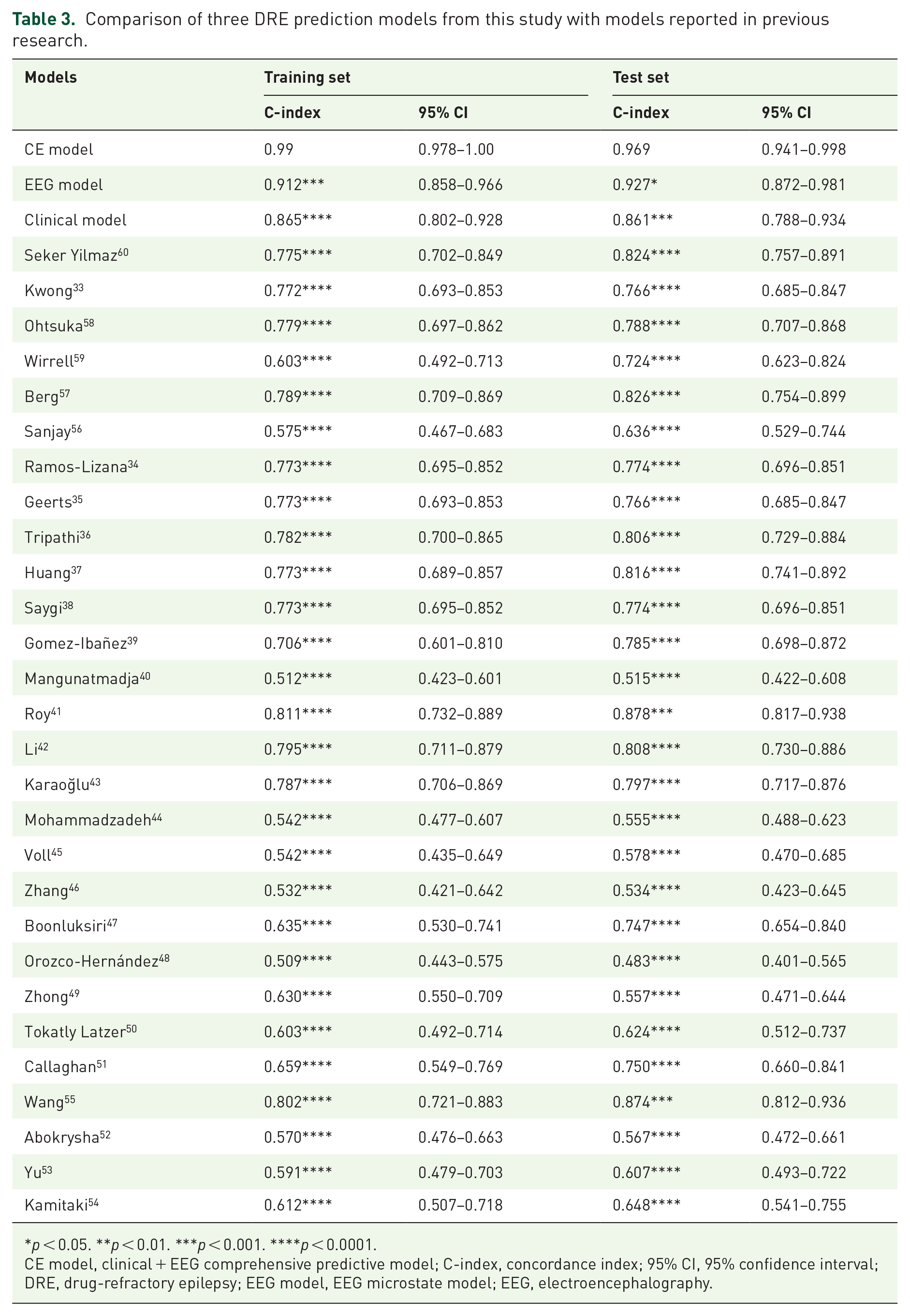
p < 0.05. **p < 0.01. ***p < 0.001. ****p < 0.0001.

CE model, clinical + EEG comprehensive predictive model; C-index, concordance index; 95% CI, 95% confidence interval; DRE, drug-refractory epilepsy; EEG model, EEG microstate model; EEG, electroencephalography.

The Brier score was used to assess the accuracy of the probability of the best-performing model, defined as the mean square deviation between the observed and predicted outcomes. The Brier scores ranged from 0 to 1.00, with 0 representing the best calibration. The Brier scores [95% confidence interval] for three models in the training set were 0.144 [0.109–0.179], 0.114 [0.075–0.152], and 0.034 [0.010–0.058]. The Brier scores [95% confidence interval] for three models in the test set were 0.144 [0.104–0.183], 0.092 [0.057–0.127], and 0.071 [0.031–0.111]. The CE model had the lowest Brier score of the three models, closest to 0, both for the training and test sets, which indicates the good performance of the constructed prediction model. Through the calibration curve, it could be observed that the predicted risk aligned well with the actual risk represented by the reference line. This indicated that the model possesses good calibration capability (Figure 5(a) and (b)).

Figure 5.

Establishment of nomograms for predicting patients with DRE: (a) calibration curve of the three models in the training set, (b) calibration curve of the three models in the test set, and (c) Nomogram for predicting patients with DRE using the duration of epilepsy, initial seizure frequency, EEG findings, absence epilepsy, comorbid depression, and the transition probability of microstates B–A, D–A, and D–B.

Then, we chose CE model as the final prediction model for DRE and further constructed a corresponding nomogram. The total nomogram score was applied to obtain the sort of probability for predicting incident DRE. The duration of epilepsy, initial seizure frequency, EEG findings, absence epilepsy, comorbid depression, and the TP of microstates B–A, D–A, and D–B were included in the nomogram (Figure 5(c)). When using the nomogram, we first needed to determine the position of different variables on their respective axes and then find the corresponding points on the top axis. After adding together the point values for all variables, we drew a vertical line downward from this total point value to predict DRE. We found that DRE was independently associated with several factors: the duration of epilepsy, initial seizure frequency, comorbid depression, and the TPs of microstates B–A, D–A, as well as D–B. The AUC values for the three models in the training set were 0.990, 0.912, and 0.865, respectively (Figure 6(a)). Similarly, the AUC values for the three models in the test set were 0.969, 0.927, and 0.861, respectively (Figure 6(b)). DCAs (Figure 6(c) and (d)) were established to confirm the clinical applicability of the nomogram. DCA showed that the prediction of DRE with the nomogram provide greater net benefits when the threshold probability was >70%.

Figure 6.

The ROC curves and DCA demonstrated the accuracy and clinical applicability of these prediction models: (a) ROC curve for the three models in the training set, (b) ROC curve for the three models in the test set, (c) decision curve for the three models in the training set, and (d) decision curve for the three models in the test set.

Discussion

Despite the development and availability of over 20 different ASMs, approximately one-third of epilepsy patients struggle to achieve seizure control through medication.^1,2 The early identification of patients developing DRE and subsequently shifting their treatment approach toward more personalized interventions, such as ketogenic diet, surgical resection, and neuromodulation therapies,³ holds significant clinical importance. To address this objective, we constructed a comprehensive predictive model based on clinical and EEG microstates features. Through C-index, AUC, calibration curve, Brier score, and DCA, this model demonstrated its superior discriminative ability, calibration, and clinical applicability. Additionally, our study innovatively visualized the application of the comprehensive prediction model through constructing a nomogram and developing a web calculator (https://fydxh.shinyapps.io/CE_model_of_DRE/), providing a novel approach for rapidly obtaining real-time predictions of the probability of DRE occurrence. In our study, a total of 45 clinical feature variables and EEG microstate feature variables were included. Correlation analysis of variables revealed correlations among some of them. To address collinearity issues and overfitting of the data, a combination of Lasso and Stepglm [both] algorithms was employed for variable selection, effectively resolving collinearity and interaction problems. Additionally, 10-fold cross validation was utilized to ensure the model’s generalization ability and accuracy. These methods contributed to constructing a simplified model, enhancing model interpretability, and optimizing overall performance.^31,32

Kuzmanovski et al.⁶¹ indicated that a longer duration of epilepsy is associated with an increased likelihood of drug resistance. Consistent with this observation, our study reports that patients diagnosed with DRE experienced epilepsy for an average of 6 years longer than those in the NDRE group. This further confirms that an extended duration of epilepsy may increase the incidence of DRE. This increase could be associated with the heightened complexity of treatment and the broader variety of ASMs used as the duration of epilepsy extends. A meta-analysis conducted in 2019 revealed that EEG abnormalities, including slow waves and epileptiform discharges, are predictive factors for DRE.⁶² Additionally, focal slowing in EEG has been demonstrated as a clinical risk factor that predicts DRE in children with cerebral palsy.⁵⁰ In this study, compared to the NDRE group, the DRE group exhibited a higher proportion of EEG with abnormal background and epileptiform discharges, consistent with the results of previous studies. This suggests that EEG abnormalities may serve as an indicator of the occurrence of DRE. The initial seizure frequency is considered a strong and independent factor in predicting the development of DRE.^37,45 Furthermore, a high seizure frequency indicates a more severe disease condition and suggests a more severe form of epilepsy.⁴³ In our study, the DRE group had a higher initial seizure frequency, consistent with the results of previous studies. This could be due to the loss of neurons in the hippocampus and the sprouting of mossy fibers caused by repeated seizures, potentially leading to the formation of recurrent excitatory circuits, thereby promoting the occurrence of DRE.⁴³

Psychological disorders are common comorbidities in patients with epilepsy, involving a range of complex neurobiological mechanisms.⁶³ Among these, depression is the most prevalent,⁶⁴ and the coexistence of depression is significantly associated with an increased risk of developing DRE.⁶⁵ In studies of patients with refractory epilepsy, about 30% of those with DRE also suffer from depression, with a prevalence rate of approximately 35% in this specific population.^22,64 This rate is significantly higher than the prevalence of depression in the general population, underscoring the importance of identifying and treating depressive disorders in patients with DRE.²² In our study, the occurrence of comorbid depression was higher among patients with DRE compared to those without DRE, consistent with past research, and further highlighted the significance of coexisting depression in the development of DRE. Kamitaki et al.⁵⁴ suggested that absence seizures serve as an independent risk factor for DRE. In our study, we found a higher proportion of absence seizures in the DRE group. The presence of absence seizures may increase the risk of developing DRE. However, further research is needed to explore the exact association between absence seizures and drug-resistant epilepsy.

Recent studies have highlighted the significant potential of EEG microstates in epilepsy and its treatment.^66,67 Jiang et al.⁶⁶ found that patients with idiopathic generalized epilepsy (IGE) who experienced seizures in the past 6 months showed higher frequencies and coverage of microstate A and lower of microstate C, with no significant differences in microstates B and D. Sun et al.⁶⁷ observed significant changes in the temporal characteristics of the four typical EEG microstates in patients with temporal lobe epilepsy and depression. Microstate A is associated with brain activity in the temporal cortex and left insula.¹⁴ Microstate B is related to the visual network,¹⁴ and an increase in the average duration of microstate B has been found to be associated with cognitive fatigue.¹⁴ Alzheimer’s disease (AD) and bipolar affective disorder are the most typical examples, with patients of both diseases showing increased connectivity in the auditory and visual networks, and cognitive impairment leading to a more visual-oriented brain activity.⁶⁸ In our study, DRE group showed increased average duration, frequency, and coverage of microstate B, while these parameters of microstate D decreased. Moreover, the TP from microstate D to B increased, consistent with previous studies. This result may reflect cognitive impairment in DRE patients due to uncontrolled long-term seizure activity, prompting a shift in brain activity toward visual functional areas. It is speculated that the frequent occurrence of microstate B in DRE patients may come at the expense of microstate D.¹⁴

Research indicates that microstate C is associated with the salience network, and a decrease in the frequency of microstate C may result from declining cognitive levels, cognitive fatigue, and epileptic seizures.⁶⁹ In our study, the duration of microstate C decreased in the DRE group, consistent with previous research, which may suggest obstacles in the patients’ cognitive-emotional assessment of the environment.⁶⁹ Abnormalities in microstate D are associated with decreased attention, and the severity of the condition is negatively correlated with the average duration and frequency of microstate D.⁷⁰ Baldini et al.⁷¹ reported a decrease in duration, coverage, and frequency of microstate D in patients with temporal lobe epilepsy, a trend also observed in our study, indicating potential attention deficits in patients with DRE. The TPs between EEG microstates are non-random and hold potential importance for understanding brain dynamics. Our study showed increased TPs (B–A, D–B) in the DRE group compared to the NDRE group, with lower transitions from D to A in the DRE group. These differences may reflect fundamental distinctions in brain activity patterns between patients with DRE and NDRE, implying different neural network dynamics and brain connectivity patterns. When combined with our previous assertion that cognitive dysfunction (reduced microstate D, increased D to B transitions) could enhance the functionality of microstate B, we can hypothesize that increased TPs from B to A may result from disease-induced dysfunctional connectivity between neural networks. This contrast with alterations in TPs from D to A and D to B could potentially enhance connectivity between microstates A and B, thereby increasing TPs.⁷⁰ These findings imply that the TPs between different microstates can all serve as important reference indicators for evaluating DRE. Future research should focus on exploring the relationship between these changes in microstate TPs and susceptibility to epileptic seizures, drug responsiveness, and brain network function.

Limitations

Our study has several limitations. First, the retrospective nature of the study introduces selection bias. To address this issue, future prospective studies are necessary. Second, our study lacks a formal power analysis for sample size calculation. Future studies should include a formal power analysis to determine the optimal sample size. Additionally, the sample size is small and limited to Asian individuals, which may affect the generalizability of our findings. Larger and multicenter studies involving diverse populations are needed. In addition, we selected other models from the PubMed database to compare with the three DRE prediction models, which may introduce selection bias. Finally, future research should focus on implementing these markers in clinical practice to establish accurate models for predicting DRE.

Conclusion

Our research shows that predicting DRE is possible using a comprehensive model that combines clinical and EEG microstate features. More evaluation is needed to determine its applicability in clinical settings.

Supplemental Material

sj-doc-1-tan-10.1177_17562864241276202 – Supplemental material for A comprehensive prediction model of drug-refractory epilepsy based on combined clinical-EEG microstate features

Supplemental material, sj-doc-1-tan-10.1177_17562864241276202 for A comprehensive prediction model of drug-refractory epilepsy based on combined clinical-EEG microstate features by Jinying Zhang, Chaofeng Zhu, Juan Li, Luyan Wu, Yuying Zhang, Huapin Huang and Wanhui Lin in Therapeutic Advances in Neurological Disorders

Supplemental Material

sj-jpg-3-tan-10.1177_17562864241276202 – Supplemental material for A comprehensive prediction model of drug-refractory epilepsy based on combined clinical-EEG microstate features

Supplemental material, sj-jpg-3-tan-10.1177_17562864241276202 for A comprehensive prediction model of drug-refractory epilepsy based on combined clinical-EEG microstate features by Jinying Zhang, Chaofeng Zhu, Juan Li, Luyan Wu, Yuying Zhang, Huapin Huang and Wanhui Lin in Therapeutic Advances in Neurological Disorders

Supplemental Material

sj-jpg-4-tan-10.1177_17562864241276202 – Supplemental material for A comprehensive prediction model of drug-refractory epilepsy based on combined clinical-EEG microstate features

Supplemental material, sj-jpg-4-tan-10.1177_17562864241276202 for A comprehensive prediction model of drug-refractory epilepsy based on combined clinical-EEG microstate features by Jinying Zhang, Chaofeng Zhu, Juan Li, Luyan Wu, Yuying Zhang, Huapin Huang and Wanhui Lin in Therapeutic Advances in Neurological Disorders

Supplemental Material

sj-tif-5-tan-10.1177_17562864241276202 – Supplemental material for A comprehensive prediction model of drug-refractory epilepsy based on combined clinical-EEG microstate features

Supplemental material, sj-tif-5-tan-10.1177_17562864241276202 for A comprehensive prediction model of drug-refractory epilepsy based on combined clinical-EEG microstate features by Jinying Zhang, Chaofeng Zhu, Juan Li, Luyan Wu, Yuying Zhang, Huapin Huang and Wanhui Lin in Therapeutic Advances in Neurological Disorders

Supplemental Material

sj-xls-2-tan-10.1177_17562864241276202 – Supplemental material for A comprehensive prediction model of drug-refractory epilepsy based on combined clinical-EEG microstate features

Supplemental material, sj-xls-2-tan-10.1177_17562864241276202 for A comprehensive prediction model of drug-refractory epilepsy based on combined clinical-EEG microstate features by Jinying Zhang, Chaofeng Zhu, Juan Li, Luyan Wu, Yuying Zhang, Huapin Huang and Wanhui Lin in Therapeutic Advances in Neurological Disorders

Footnotes

Acknowledgements

We are grateful to all the participants for their valuable information, cooperation, and participation.

Declarations

ORCID iD

Wanhui Lin

Supplemental material

Supplemental material for this article is available online.

References

Janmohamed

Brodie

Kwan

Pharmacoresistance - Epidemiology, mechanisms, and impact on epilepsy treatment. Neuropharmacology 2020; 168: 107790.

Kwan

Arzimanoglou

Berg

, et al. Definition of drug resistant epilepsy: consensus proposal by the ad hoc Task Force of the ILAE Commission on Therapeutic Strategies [published correction appears in Epilepsia 2010; 51(9): 1922]. Epilepsia 2010; 51(6): 1069–1077.

Anyanwu

Motamedi

GK.

Diagnosis and surgical treatment of drug-resistant epilepsy. Brain Sci 2018; 8(4): 49.

Wirrell

EC.

Predicting pharmacoresistance in pediatric epilepsy. Epilepsia 2013; 54(Suppl. 2): 19–22.

Asadi-Pooya

Brigo

Lattanzi

, et al. Adult epilepsy. Lancet 2023; 402(10399): 412–424.

Antonakakis

Dimitriadis

Zervakis

, et al. Aberrant whole-brain transitions and dynamics of spontaneous network microstates in mild traumatic brain injury. Front Comput Neurosci 2020; 13: 90.

Tait

Zhang

+microstate: a MATLAB toolbox for brain microstate analysis in sensor and cortical EEG/MEG. Neuroimage 2022; 258: 119346.

Koenig

Marti-Lopez

Valdes-Sosa

Topographic time-frequency decomposition of the EEG. Neuroimage 2001; 14(2): 383–390.

Cao

Zhao

Shan

, et al. Brain functional and effective connectivity based on electroencephalography recordings: a review. Hum Brain Mapp. 2022; 43(2): 860–879.

10.

Khanna

Pascual-Leone

Michel

, et al. Microstates in resting-state EEG: current status and future directions. Neurosci Biobehav Rev 2015; 49: 105–113.

11.

Gao

Jia

, et al. Altered resting-state EEG microstate parameters and enhanced spatial complexity in male adolescent patients with mild spastic diplegia. Brain Topogr 2017; 30(2): 233–244.

12.

Michel

Koenig

EEG microstates as a tool for studying the temporal dynamics of whole-brain neuronal networks: a review. Neuroimage 2018; 180(Pt B): 577–593.

13.

Koenig

Prichep

Lehmann

, et al. Millisecond by millisecond, year by year: normative EEG microstates and developmental stages. Neuroimage 2002; 16(1): 41–48.

14.

Wang

Yin

Progress in the Analysis and application of microstates in electroencephalography. J Biomed Eng 2023; 40(01): 163–170.

15.

Britz

Van De Ville

Michel

CM.

BOLD correlates of EEG topography reveal rapid resting-state network dynamics. Neuroimage 2010; 52(4): 1162–1170.

16.

Yuan

Zotev

Phillips

, et al. Spatiotemporal dynamics of the brain at rest–exploring EEG microstates as electrophysiological signatures of BOLD resting state networks. Neuroimage 2012; 60(4): 2062–2072.

17.

Vaughan

Jr.

The neural origins of human event-related potentials. Ann N Y Acad Sci 1982; 388: 125–138.

18.

Irisawa

Isotani

Yagyu

, et al. Increased omega complexity and decreased microstate duration in nonmedicated schizophrenic patients. Neuropsychobiology 2006; 54(2): 134–139.

19.

Nishida

Morishima

Yoshimura

, et al. EEG microstates associated with salience and frontoparietal networks in frontotemporal dementia, schizophrenia and Alzheimer’s disease. Clin Neurophysiol 2013; 124(6): 1106–1114.

20.

Drissi

Szakács

Witt

, et al. Altered brain microstate dynamics in adolescents with narcolepsy [published correction appears in Front Hum Neurosci 2019 Nov 06; 13: 385]. Front Hum Neurosci 2016; 10: 369.

21.

Liu

Tang

Wei

, et al. Altered peri-seizure EEG microstate dynamics in patients with absence epilepsy. Seizure 2021; 88: 15–21.

22.

Cao

Sun

, et al. Potential clinical and biochemical markers for the prediction of drug-resistant epilepsy: a literature review. Neurobiol Dis 2022; 174: 105872.

23.

Jia

Wang

Huang

, et al. A comparison of the Mini-Mental State Examination (MMSE) with the Montreal Cognitive Assessment (MoCA) for mild cognitive impairment screening in Chinese middle-aged and older population: a cross-sectional study. BMC Psychiatry 2021; 21(1): 485.

24.

Tang

, et al. Influencing factors for prenatal stress, anxiety and depression in early pregnancy among women in Chongqing, China. J Affect Disord 2019; 253: 292–302.

25.

Nagabhushan Kalburgi

Kleinert

Aryan

, et al. MICROSTATELAB: the EEGLAB toolbox for resting-state microstate analysis. Brain Topogr. Epub ahead of print September 11, 2023. DOI: 10.1007/s10548-023-01003-5.

26.

Delorme

Makeig

EEGLAB: an open source toolbox for analysis of single-trial EEG dynamics including independent component analysis. J Neurosci Methods 2004; 134(1): 9–21.

27.

Zhu

Wei

, et al. Intrinsic brain activity differences in perampanel-responsive and non-responsive drug-resistant epilepsy patients: an EEG microstate analysis. Ther Adv Neurol Disord 2024; 17: 17562864241227293.

28.

Cai

Chen

, et al. Altered resting-state EEG microstate in idiopathic sudden sensorineural hearing loss patients with tinnitus. Front Neurosci 2019; 13: 443.

29.

Kikuchi

Koenig

Munesue

, et al. EEG microstate analysis in drug-naive patients with panic disorder. PLoS One 2011; 6(7): e22912.

30.

Pascual-Marqui

Michel

Lehmann

Segmentation of brain electrical activity into microstates: model estimation and validation. IEEE Trans Biomed Eng 1995; 42(7): 658–665.

31.

Wang

, et al. Methods and comparison of variable selection in clinical prediction models [J]. Modern Trad Chin Med Clin 2024; 31(02): 6–12.

32.

Liang

Lai

, et al. Evaluation of predictive model generalization capability and its implementation in R software using 10-fold cross-validation. Chin Hospital Stat 2020; 27(4): 289–292.

33.

Kwong

Sung

Wong

, et al. Early predictors of medical intractability in childhood epilepsy. Pediatr Neurol 2003; 29(1): 46–52.

34.

Ramos-Lizana

Aguilera-López

Aguirre-Rodríguez

, et al. Early prediction of refractory epilepsy in childhood. Seizure 2009; 18(6): 412–416.

35.

Geerts

Arts

Stroink

, et al. Course and outcome of childhood epilepsy: a 15-year follow-up of the Dutch Study of Epilepsy in Childhood. Epilepsia 2010; 51(7): 1189–1197.

36.

Tripathi

Padhy

Vibha

, et al. Predictors of refractory epilepsy in north India: a case-control study. Seizure 2011; 20(10): 779–783.

37.

Huang

, et al. A predictive risk model for medical intractability in epilepsy. Epilepsy Behav 2014; 37: 282–286.

38.

Saygi

Erol

Alehan

Early clinical predictors of intractable epilepsy in childhood. Turk J Med Sci 2014; 44(3): 490–495.

39.

Gomez-Ibañez

McLachlan

Mirsattari

, et al. Prognostic factors in patients with refractory idiopathic generalized epilepsy. Epilepsy Res 2017; 130: 69–73.

40.

Mangunatmadja

Indra

Widodo

, et al. Risk factors for drug resistance in epileptic children with age of onset above five years: a case-control study. Behav Neurol 2021; 2021: 9092824.

41.

Roy

Ronquillo

Ladino

, et al. Risk factors associated with drug resistant focal epilepsy in adults: a case control study. Seizure 2019; 73: 46–50.

42.

Chen

, et al. Treatment outcome and risk factors of adult newly diagnosed epilepsy: a prospective hospital-based study in Northeast China. Front Neurol 2021; 12: 747958.

43.

Karaoğlu

Yasş

Polat

Aİ

, et al. Clinical predictors of drug-resistant epilepsy in children. Turk J Med Sci 2021; 51(3): 1249–1252.

44.

Mohammadzadeh

Nazarbaghi

The prevalence of drug-resistant-epilepsy and its associated factors in patients with epilepsy. Clin Neurol Neurosurg 2022; 213: 107086.

45.

Voll

Hernández-Ronquillo

Buckley

, et al. Predicting drug resistance in adult patients with generalized epilepsy: a case-control study. Epilepsy Behav 2015; 53: 126–130.

46.

Zhang

, et al. A prospective cohort study of prognosis for newly diagnosed epilepsy in east China. BMC Neurol 2013; 13: 116.

47.

Boonluksiri

Visuthibhan

Katanyuwong

Clinical prediction rule of drug resistant epilepsy in children. J Epilepsy Res 2015; 5(2): 84–88.

48.

Orozco-Hernández

Quintero-Moreno

Marín-Medina

, et al. Multivariable prediction model of drug resistance in adult patients with generalized epilepsy from Colombia: a case-control study. Epilepsy Behav 2018; 88: 176–180.

49.

Zhong

Chen

, et al. Psychiatric symptoms predict drug-resistant epilepsy in newly treated patients. Seizure 2022; 103: 86–91.

50.

Tokatly Latzer

Blumovich

Sagi

, et al. Prediction of drug-resistant epilepsy in children with cerebral palsy. J Child Neurol 2020; 35(3): 187–194.

51.

Callaghan

Schlesinger

Rodemer

, et al. Remission and relapse in a drug-resistant epilepsy population followed prospectively. Epilepsia 2011; 52(3): 619–626.

52.

Abokrysha

Taha

Shamloul

, et al. Clinical, radiological and electrophysiological predictors for drug-resistant epilepsy. Egypt J Neurol Psychiatr Neurosurg 2023; 59(1): 44.

53.

Liu

Sun

, et al. Risk factors for Drug-resistant Epilepsy (DRE) and a nomogram model to predict DRE development in post-traumatic epilepsy patients. CNS Neurosci Ther 2022; 28(10): 1557–1567.

54.

Kamitaki

Janmohamed

Kandula

, et al. Clinical and EEG factors associated with antiseizure medication resistance in idiopathic generalized epilepsy. Epilepsia 2022; 63(1): 150–161.

55.

Wang

Han

Yang

, et al. An integrative prediction algorithm of drug-refractory epilepsy based on combined clinical-EEG functional connectivity features. J Neurol 2022; 269(3): 1501–1514.

56.

Chawla

Aneja

Kashyap

, et al. Etiology and clinical predictors of intractable epilepsy. Pediatric Neurol 2002; 27(3): 186–191.

57.

Berg

Shinnar

Levy

, et al. Early development of intractable epilepsy in children: a prospective study [published correction appears in Neurology 2001 Sep 11; 57(5): 939]. Neurology 2001; 56(11): 1445–1452.

58.

Ohtsuka

Yoshinaga

Kobayashi

, et al. Predictors and underlying causes of medically intractable localization-related epilepsy in childhood Pediatr Neurol 2001; 24(3): 209–213.

59.

Wirrell

Wong-Kisiel

Mandrekar

, et al. Predictors and course of medically intractable epilepsy in young children presenting before 36 months of age: a retrospective, population-based study. Epilepsia 2012; 53(9): 1563–1569.

60.

Seker Yilmaz

Okuyaz

Komur

. Predictors of intractable childhood epilepsy. Pediatr Neurol 2013; 48(1): 52–55.

61.

Kuzmanovski

Cvetkovska

Babunovska

, et al. Seizure outcome following medical treatment of mesial temporal lobe epilepsy: clinical phenotypes and prognostic factors. Clin Neurol Neurosurg 2016; 144: 91–95.

62.

Xue-Ping

Hai-Jiao

Li-Na

, et al. Risk factors for drug-resistant epilepsy: a systematic review and meta-analysis. Medicine (Baltimore) 2019; 98(30): e16402.

63.

Hitiris

Mohanraj

Norrie

, et al. Predictors of pharmacoresistant epilepsy. Epilepsy Res 2007; 75(2–3): 192–196.

64.

D’Alessio

Mesarosova

Anink

, et al. Reduced expression of the glucocorticoid receptor in the hippocampus of patients with drug-resistant temporal lobe epilepsy and comorbid depression. Epilepsia 2020; 61(8): 1595–1605.

65.

Scévola

Sarudiansky

Lanzillotti

, et al. To what extent does depression influence quality of life of people with pharmacoresistant epilepsy in Argentina?. Epilepsy Behav 2017; 69: 133–138.

66.

Jiang

Zhu

, et al. Altered resting-state electroencephalography microstates in idiopathic generalized epilepsy: a prospective case–control study. Front Neurol 2021; 12: 710952.

67.

Sun

Ren

, et al. Intrinsic brain activity in temporal lobe epilepsy with and without depression: insights from EEG microstates. Front Neurol 2021; 12: 753113.

68.

Vellante

Ferri

Baroni

, et al. Euthymic bipolar disorder patients and EEG microstates: a neural signature of their abnormal self-experience?. J Affect Disord 2020; 272: 326–334.

69.

Chu

Wang

Cai

, et al. Spatiotemporal EEG microstate analysis in drug-free patients with Parkinson’s disease. NeuroImage Clin 2020; 25: 102132.

70.

Fang

Zhu

Zhang

, et al. EEG microstates in epilepsy with and without cognitive dysfunction: alteration in intrinsic brain activity. Epilepsy Behav 2024; 154: 109729.

71.

Baldini

Duma

Danieli

, et al. Electroencephalographic microstates as a potential neurophysiological marker differentiating bilateral from unilateral temporal lobe epilepsy. Epilepsia 2024; 65: 664–674.

Supplementary Material

Please find the following supplemental material available below.

For Open Access articles published under a Creative Commons License, all supplemental material carries the same license as the article it is associated with.

For non-Open Access articles published, all supplemental material carries a non-exclusive license, and permission requests for re-use of supplemental material or any part of supplemental material shall be sent directly to the copyright owner as specified in the copyright notice associated with the article.

0.00 MB

0.09 MB

0.88 MB

0.90 MB

10.55 MB

0.07 MB