Sage Journals: Discover world-class research

Abstract

Team tactical behaviour in football can be analysed using positional data. Global navigation satellite systems (GNSS) track players’ positions on the pitch and provide data on latitude and longitude positioning. However, data pre-processing is required for GNSS positional data prior to tactical analysis, which varies across studies and is scarcely reported. This lack of standardisation poses a challenge to the application and reproducibility of earlier findings. Therefore, Study 1 aimed to establish an analytical pipeline for tactical analysis, addressing typical data processing issues. Study 2 aimed to deploy this pipeline as a proof of concept, comparing team tactical behaviour across in-possession, out-of-possession, and transition phases in a competitive match. Independent positional datasets from different GNSS devices were used in two studies. Study 1 presented an analytical pipeline providing solutions for map projection, rotation matrix application, and handling missing values in data from small-sided games. Study 2 applied the pipeline to match data and revealed significant differences in team tactical behaviour across match phases. The analytical pipeline demonstrated its generalisability to match and training scenarios as well as across different tracking devices, allowing practitioners and scientists to advance tactical analysis in team sports using player tracking technology. This pipeline warrants disclosing processing procedures and the synchronisation of positional and event data to improve the reliability of findings.

Keywords

football analytics collective behaviour GPS match phase soccer

Introduction

In recent years, the application of modern player tracking technologies in football (soccer or association football) has enabled in-depth analyses of individual contributions and team dynamics.¹ This technological evolution encompasses player tracking technologies with Global Navigation Satellite Systems (GNSS), Local Positioning Measurement systems (LPM), and optical tracking systems, which can capture players’ positional information to study football performance, such as collective tactical behaviour.² While LPM and optical tracking systems capture players’ positions in Cartesian coordinates (i.e., x- and y- coordinates), with high accuracy and higher sampling frequency, making the positional data directly suitable for tactical analysis,² their widespread use in football is limited by the associated high costs, infrastructure requirements for installation, and lack of portability.³

Conversely, wearable tracking systems using GNSS technology feature cost-effectiveness and portability,³ enabling the wide application for physical and tactical performance analysis across playing levels and age groups.⁴ However, the positional data from GNSS are captured in geographic coordinates (i.e., latitude and longitude) and require additional data processing before calculating meaningful tactical measures (Figure 1). These “intrinsic shortcomings” have led to GNSS player tracking technologies being mainly used for locomotor analysis (e.g., distance in specific speed zones), while LPM and optical-tracking data remain the preferred options for tactical analysis. Consequently, tactical analysis in football is dominated by a small number of research groups with access to expensive equipment or affiliations with football clubs providing optical-tracking data. In turn, open analysis packages with widespread use in the community are also based on data from LPM and optical tracking systems.^5–7 A comprehensive processing pipeline can enable the use of GNSS data in a similar fashion and make tactical analysis more accessible for research and less-wealthy team sport federations and clubs.

Figure 1.

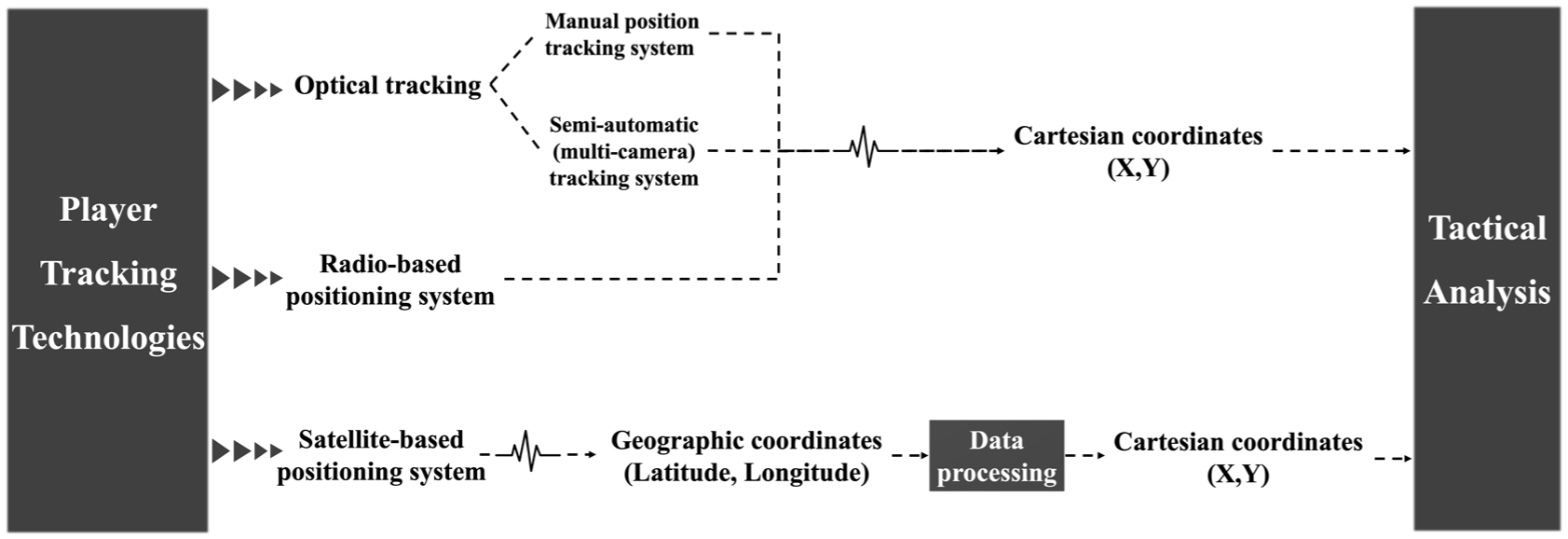
Mainstream player tracking technology systems that provide position information of moving objects, and types of generated raw data. Geographic coordinates require extra data processing prior to tactical analysis.

GNSS is an umbrella term for various satellite navigation systems,⁸ including GPS, with manufacturers typically integrating multiple systems to enhance data reliability and validity,⁹ Despite its advantages, challenges such as missing data¹⁰ and synchronisation issues typically persist in analysing positional data from GNSS devices for tactical purposes.¹¹ Furthermore, it requires additional information on the pitch location and orientation.¹² While some guidance on preparing GNSS positional data has been provided by Folgado et al.,¹² the scarcity of reported workflows raises concerns about the consistency and comparability of findings across studies. The increasing popularity of wearable technology for analysing collective behaviour^13–15 warrants a transparent analytical pipeline, ensuring data quality and amplifying insights into team dynamics.

Team tactical performance in football is defined by how teams manage space and time through individual and collective actions.^16–18 Tactical measures derived from positional data offer insights into intra-team coordination and inter-team competition and unveil strengths and weaknesses in positioning and interaction.^2,19,20 However, a lack of standardisation in analysing team tactical performance persists across studies, due to a variety of approaches.^21,22 A universal working pipeline could also benefit coaching strategy (e.g., analysing historical performance against a specific opposition) and long-term player development.

Therefore, this manuscript addresses two objectives, each presented in a study. Study 1 aims to establish a universal working pipeline for tactical analysis using GNSS tracking systems, addressing the gaps in analytical workflows identified from previous studies. Study 2 deploys the analytical pipeline to match data as a proof of concept for this pipeline and explores variations in team tactical behaviour across match phases, contributing to the understanding of dynamic team behaviour. To underscore the pipeline’s applicability, a step-by-step workflow is provided and applied to two independent datasets from different versions of GNSS units in two studies. All processing steps and the corresponding code are available on an open access repository (https://osf.io/d5meq/?view_only).

Study 1: Analytical pipeline for tactical analysis using GNSS positional data

Materials

Data from Spanish male academy players (under-18) were collected during 6 versus 6 + goalkeepers small-sided games (SSGs). Positional data were collected with Catapult Optimeye S5 tracking devices (10 Hz, Catapult Innovations, South Melbourne, VIC, Australia). Deidentified data from all players were compiled into a data repository for secondary data analysis.

Preprocessing

Tactical analysis using positional data involves three data sources: A) positional data in geographic coordinates; B) session plan with details on time and outfield players; C) pitch coordinates. Datasets A–C are used at various stages in the data processing (Figure 2).

Figure 2.

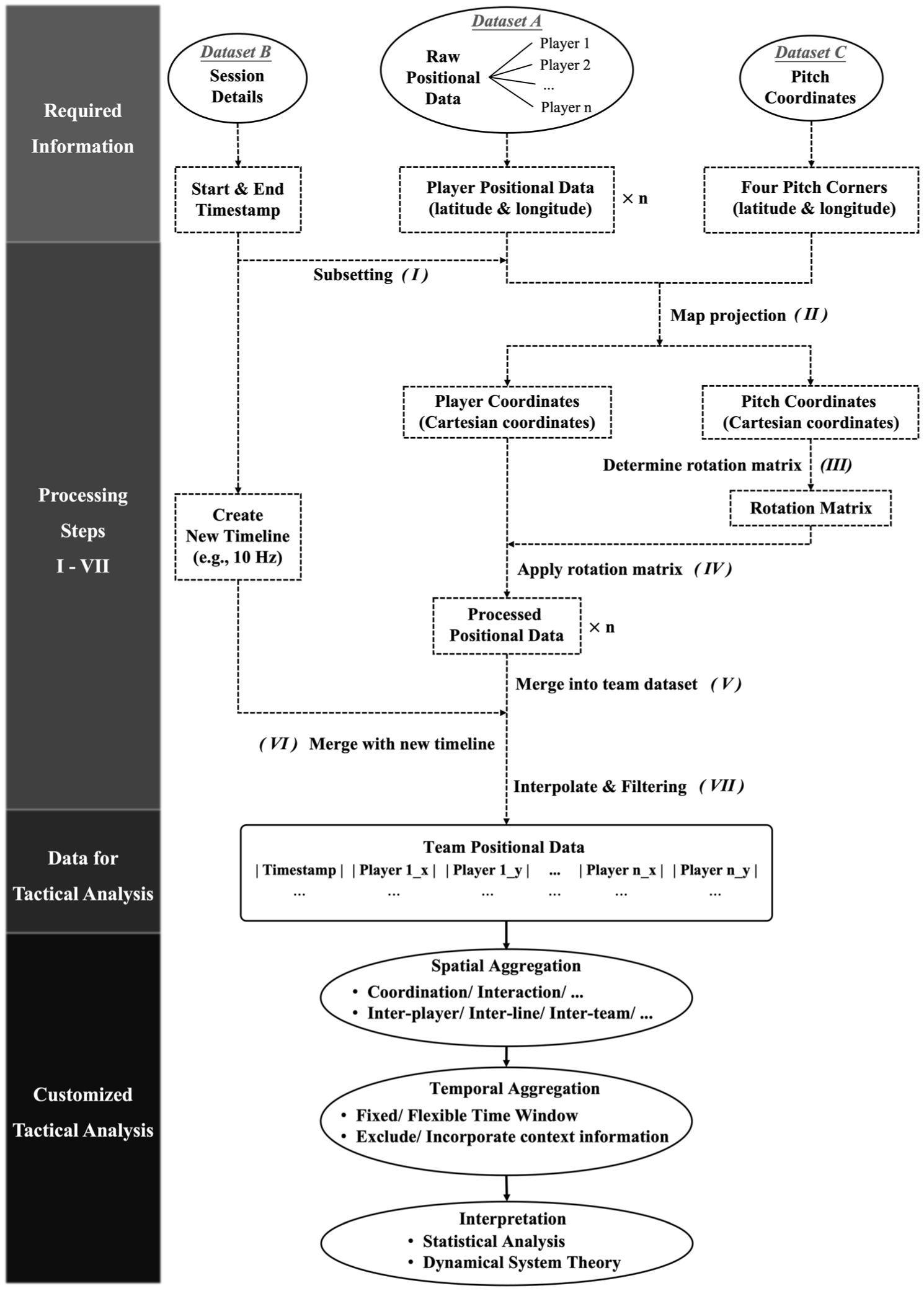
Analytical pipeline of preparing GNSS positional data for tactical analysis.

Dataset A contains the raw export of positional data from GNSS player tracking technology, including timestamps and latitude and longitude coordinates. Missing data and data noise may exist in these individual datasets, which will be addressed in the pipeline.

Dataset B includes session details with the start and end timestamps of the activity (e.g., match halves, training drills), facilitating exclusion of non-match or non-training activities from positional data (Step I).

Dataset C includes pitch location details, necessary for orientating positional data. In practice, two viable methods for retrieving the pitch location can be considered: using web mapping platforms (e.g., Google Maps) or relying on GNSS tracking devices. A pilot test demonstrated the stability and effectiveness of web mapping (see Supplemental Documents). This method proved accessible and spared the need for additional data processing as would be inevitable with using GNSS tracking devices. While GNSS devices can also provide pitch coordinates and may serve as a viable alternative for situations involving unmarked training pitches or partly obstructed stadium areas, data from GNSS showed relatively large variability during collection (see Supplemental Documents). Given these considerations, the web mapping protocol for pitch location data was adopted in this study.

Working pipeline

All procedures were conducted in Python 3.8 and the customised Python routines along with sample datasets are accessible via https://osf.io/d5meq/?view_only for transparency and reproducibility. The repository contains two Python files: all functions used in file 1 (main analysis) were detailed in file 2 (preprocessing). The stepwise analytical pipeline is outlined below and represented in Figure 2.

Step I. Data subsetting

A match or training session usually starts after activation of GNSS units and stops before deactivation. This common practice captures noise of activities unrelated to match-play or training. Therefore, it is necessary to extract the positional data of interest from the raw dataset based on the start and end timestamps of the session details (dataset B). The Unix-formatted timestamps, representing the precise date and time of each activity, serve as reference for this extraction process. See corresponding codes from line 177 (file 1) and line 675 to 740 (file 2).

Step II. Map projection

The transformation of geographic coordinates from datasets A and C to Cartesian coordinates is achieved through map projection. Various mathematical models such as the Stereographic double projection, Lambert conical projection, Transverse Mercator Projection (Gauss-Krüger projection), and Universal Transverse Mercator system (UTM, developed based on Transverse Mercator), were considered.^23–25 Detailed mathematical formulas and equations are elaborated in the cited literature. The accuracy of some methods depends on the region that is being mapped. The UTM, recognised for its high accuracy and global applicability,^26,27 was applied in this study. This projection has been outlined in file 2 (line 267–331).

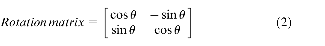
Step III. Rotation matrix

Positional data are often collected from different locations, such as home and away matches or training pitches, resulting in different orientations of pitch and positional data. For tactical analysis purposes, it is crucial to align the pitch length and width with the x and y axes respectively, allowing for coherent goal-to-goal or side-to-side representations²⁸ and the integration with video data. Folgado et al.¹² proposed that a rotational adjustment is necessary, involving either clockwise or counterclockwise rotation dependent on the specific pitch orientation (Figure 3).

Figure 3.

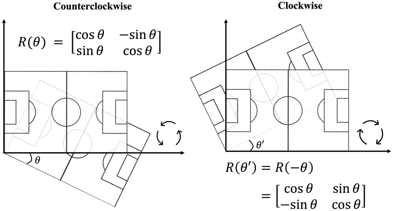
Two types of rotation and corresponding rotation matrices.

The stepwise procedure for calculating the rotation matrix is as follows: (1) Establish an origin for pitch coordinate system, typically the lower left vertex of pitch; (2) Identify another vertex on the pitch length that should be parallel to the x-axis after rotation; (3) Determine the angle between the pitch length and the x-axis¹²; (4) Calculate the rotation matrix using the determined angle $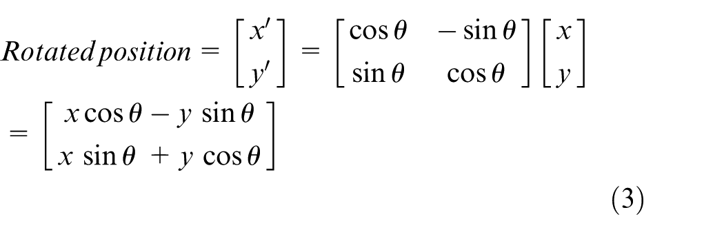θ$ , as shown in Figure 3 (Step III). These steps have been outlined in file 1 (line 123–146) and file 2 (line 372–466).

Step IV. Calibrate positional data (application of rotation matrix)

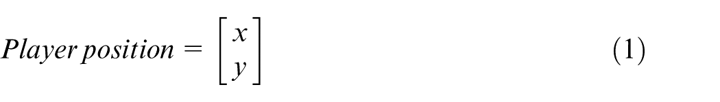
Players’ positional data are subsequently rotated with the established rotation matrix, aligning players’ positions to the x and y axes.¹² Each player’s position at every timestamp is expressed as a column vector containing x-coordinate and y-coordinate (equation (1)). The rotation matrix is a 2 × 2 matrix with angle $θ$ (equation (2)). As shown in Figure 3, the rotation is counterclockwise if $θ$ is positive and clockwise if $θ$ is negative. The resulting rotated position is derived through the dot product of these arrays (equation (3)), with the first element as the processed x-coordinate ( $x'$ ) and the second as the processed y-coordinate ( $y'$ ). This transformation ensures that positional data align with the adjusted coordinate system, facilitating accurate and standardised spatial analysis. This step has been outlined file 2 (line 469–475).

Player position = [\begin{matrix} x \\ y \end{matrix}]

(1)

Rotation matrix = [\begin{matrix} \cos θ & - \sin θ \\ \sin θ & \cos θ \end{matrix}]

(2)

\begin{matrix} Rotated position = [\begin{matrix} x' \\ y' \end{matrix}] = [\begin{matrix} \cos θ & - \sin θ \\ \sin θ & \cos θ \end{matrix}] [\begin{matrix} x \\ y \end{matrix}] \\ = [\begin{matrix} x \cos θ - y \sin θ \\ x \sin θ + y \cos θ \end{matrix}] \end{matrix}

(3)

Step V. Integration into team positional dataset

To facilitate team tactical analysis, the rotated Cartesian coordinates of each player are merged into a team positional dataset. This merging process is based on the “timestamp” column, utilising a full outer join approach to preserve the union of keys from all frames (Figure 4(a)). This approach ensures that all original data points are present in the merged dataset, effectively synchronising the players’ data. This step has been outlined in file 2 (line 800–804). Although it is expected that players have a similar data volume, in reality, the number of observations within individual datasets may vary due to signal instability.

Figure 4.

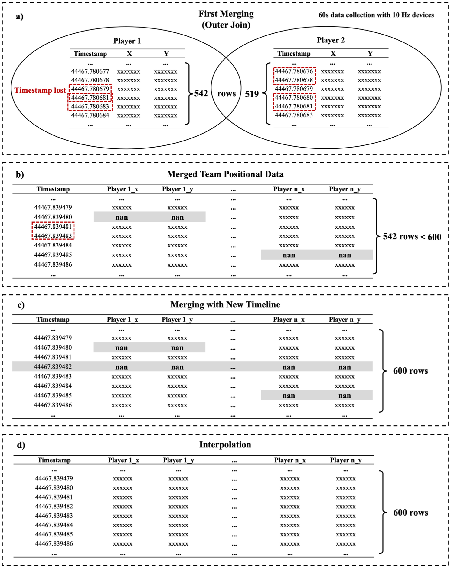
Details of exemplar datasets processed from individual positional data to ready-to-use team positional data, including (a) merging individual data, (b) merged team data, (c) merging with new timeline, and d) interpolation.

Step VI. Identifying missing data

Upon merging players’ data into the team positional dataset, the potential emergence of missing data (i.e., NaN or null value in Figure 4(b)) requires careful consideration. Positional data from GNSS may contain occasional gaps for individual players. This individual data loss could also be identified and resampled. First, the difference between the total observations in the dataset and the expected number of observations should be identified. For example, in the scenario that positional data collected with 10-Hz devices for 60 s, there are supposed to be 600 observations in the dataset (i.e., 60 s × 10 Hz = 600 data points). If there are fewer than 600 data points, this suggests data loss that needs to be addressed.

Second, before the data can be resampled, a full timeline should be created. A pragmatic solution is to create a dummy timeline using start and end timestamps from the session details (dataset B) and then merge the generated timeline with team positional data. This approach ensures proceeding with a complete timeline of 10 Hz positional data (Figure 4(c)) and ensures synchronisation of data across players. Creating a dummy timeline and merging steps have been outlined in file 2 (line 819–877) and file 1 (line 191), respectively.

Step VII. Resampling through interpolation and filtering

As a result of step VI, missing data has been identified as partial or complete data loss at timestamps (Figure 4). Partial data loss indicates missing positional data for some players’ data but not for all, while complete data loss signifies missing positional data for all players at specific timestamps. While these instances may seem significant for positional data quality, the associated consequences might be relatively marginal, as outlined below.

In the exemplar dataset, approximately 40% of all observations contained partial data loss, with a maximum of five continuous observations (i.e., consecutive data loss of 0.5 s) with null values identified for a single player. Furthermore, 13.6% of timestamps were lost concurrently for the whole team (i.e., complete data loss). Importantly, no instance of continuous missing timestamps was found in the exemplar data, limiting complete data loss to only 0.1 s. Although data loss should be minimised during data collection, partial interpolation is a viable solution for further processing and analysis. The code for checking data loss has been outlined in file 2 (line 881–974).

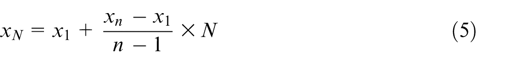
Mathematical interpolation, a technique for estimating and filling in null values based on known data points,²⁹ was applied in this study for data resampling. Missing x-coordinates and y-coordinates were interpolated using linear interpolation, for data points in one spatial dimension (Figure 4(d)). For example, to estimate these n−1 continuous missing data points in equation (4), the Nth missing data point X_N can be retrieved by equation (5) and filled into the data sequence. Accordingly, the reliability of the interpolation increases with fewer continuous missing data points.

Dataset = {x_{1}, NaN, \dots, NaN, x_{n}}

(4)

x_{N} = x_{1} + \frac{x_{n} - x_{1}}{n - 1} \times N

(5)

The accuracy of positional data from the GNSS tracking technology is susceptible to external factors. To increase data accuracy, the Savitzky-Golay filter³⁰ and Butterworth low-pass filter¹² were introduced to smooth positional data in football tactical analysis. Both have been made available in the code for user selection. Interpolation (line 195) and data smoothing (line 199–203) steps have been outlined in file 1.

Customised tactical analysis

As outlined in Figure 2, GNSS positional data are thoroughly processed within the analytical pipeline, facilitating further tactical analysis. Tactical measures can be calculated at individual, sub-group, and team levels to characterise spatial coordination and interaction patterns. Various time windows can be applied to aggregate spatial measures temporally. The type and amount of information involved characterises each time window. In the following case study, match-phase information will be used to analyse team tactical behaviour in different phases of the official match. This case study serves to validate the effectiveness of the analytical pipeline (face validation) and provides a proof of concept for its application in examining collective behaviour in football.

Study 2: A case study on comparing team tactical behaviour across match phases

Materials

Positional data of 13 professional football players (10 starting outfield players and three substitutes; mean ± SD: age = 26.3 ± 2.4 years; professional playing experience = 4.7 ± 1.5 years) during one competitive match were collected using Catapult Vector S7 devices (10 Hz, Catapult Innovations, Melbourne, VIC, Australia). The goalkeeper was excluded from the analysis. All players belonged to the first team competing in the English Championship during the 2020/2021 season. The reliability of the current device has been previously tested.³¹ Match video footage was used to annotate match phases (i.e., in-possession, out-of-possession, and two transition phases). Annotation was performed by an experienced and professional analyst using Hudl Sportscode³²—a dedicated tool for football notational analysis^11,33—to record the time point of switches in match phases, according to the definition of match phases (Table 1). Deidentified data from all players were compiled into a data repository. No ethical approval was deemed necessary by the local ethical board for this secondary data analysis.

Table 1.

Definition of open-play match phases as used by the team’s analyst.

Phases	Definition (starting point)
In possession	HT controls ball possession, originating from transitions or restarts
Defence-to-attack transition	HT regains ball possession
Out of possession	OT controls ball possession, originating from transitions or restarts
Attack-to-defence transition	OT regains ball possession

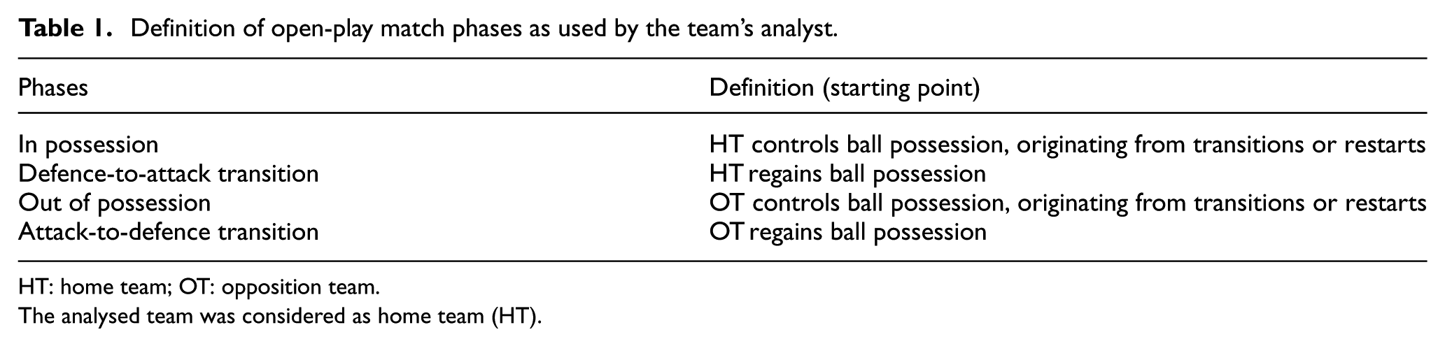
HT: home team; OT: opposition team.

The analysed team was considered as home team (HT).

The effective playing time comprised various match phases, each corresponding to different ball possession scenarios. The phases included in-possession (IP), out-of-possession (OOP), attack-to-defence transition (ADT), and defence-to-attack transition (DAT) phases. To illustrate, DAT begins after regaining the ball from an interception, tackle, or duel. The team can attempt to progress towards the opponent’s goal in a quick and incisive manner or to consolidate possession against counterpressure. IP is considered as a possession sequence, with the team in control of the ball, which is typically illustrated as a series of uninterrupted on-the-ball events by the team.³⁴ If multiple ball turnovers occur in a short period of time with little attempt to consolidate possession, it is considered as unstructured phases instead of regaining. Those unstructured phases are excluded from further data analysis. DAT ends when 1) the team consolidates possession (i.e., IP), or 2) the opposing team regains the ball (i.e., ADT).

Data processing

Datasets

Following the pipeline presented in Study 1, dataset-S2-A corresponded to GNSS positional data of all players. Dataset-S2-B comprised match phase data. Dataset-S2-C contained geographic coordinates of the pitch location retrieved from a web mapping platform. The analytical pipeline from Study 1 was applied to prepare positional data for tactical analysis. No data loss was found in dataset-S2-A. The Savitzky-Golay filter was used for data smoothing. All the processing was conducted in Python 3.8, using the aforementioned preprocessing script.

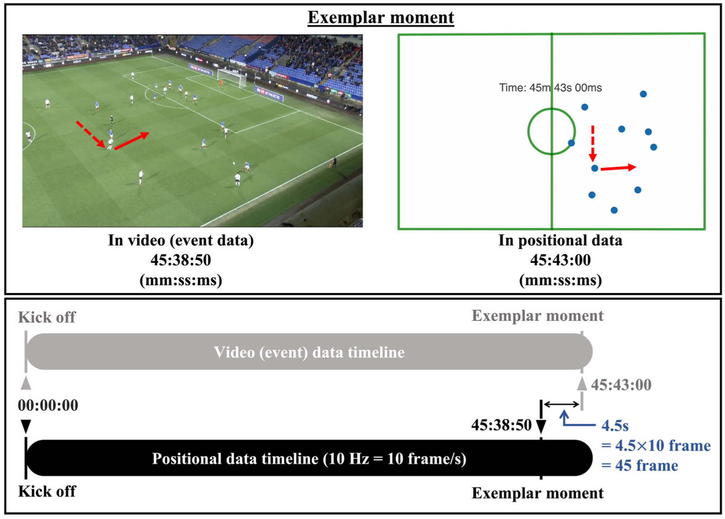
A systematic offset between the positional and event data was detected in dataset-S2-A and dataset-S2-B. Visual inspection of the video and positional data, with start and end times highlighted, showed that the positional data and event data showed misalignment. This misalignment is a recognised issue when positional and event data are integrated.^11,35 A systematic offset correction was applied for each half independently, with a further correction at the end of each half to address drift (Figure 5). To verify synchronisation, several moments were randomly selected for visual inspection after corrections, which confirmed that timelines were aligned along the entire match.

Figure 5.

After determining and synchronising start timestamps, exemplar moments were selected to compare end timestamps in two types of data. The same lag was detected in both halves and might be caused by the playing speed of video footage differing from the sampling rate of positional data.

Team tactical behaviour

Processed team positional data were used to calculate the following tactical measures: centroid, length, width, length per width (LpW) ratio, surface area, lateral and longitudinal stretch indices, and interpersonal distance (ID) of team members (Figure 6). The mean lateral and longitudinal position of all outfield players was determined as the team centroid.³⁶ Stretch indices (longitudinal and lateral) were the average distance of each player to the centroid in longitudinal and lateral directions.³⁷ The surface area referred to the convex hull enclosed by outfield players.³⁶ All measures were calculated on the team level at each timestamp and averaged for duration within each phase.

Figure 6.

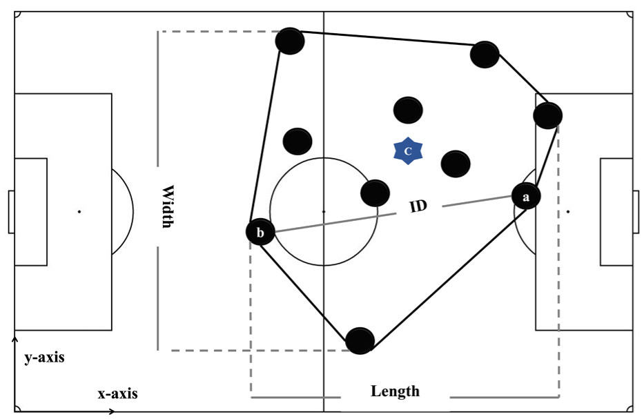
Tactical measures illustration. C exemplifies the team centroid. $Length = x_{\max} - x_{\min}$ , $width = y_{\max} - y_{\min}$ , $LpW = Length / Width$ , $ID = \sqrt{{(x_{a} - x_{b})}^{2} + {(y_{a} - y_{b})}^{2}}$ .

Statistical analysis

Team tactical measures were considered as dependent variables and compared across match phases (IP, OOP, DAT, and ADT) using a one-way ANOVA and Welch’s test due to unequal variances. Significance level was set at 5%. Eta squared (η²) was calculated as the effect size. For interpretation, magnitudes of the effect size were considered as small (η² < 0.06), moderate (0.06 ≤ η² < 0.15), or large (η² ≥ 0.15).³⁸ Pairwise comparison (Tamhane’s post-hoc test) was conducted to determine significant difference between phases, given unequal variances.³⁹ Cohen’s d was determined as effect size for pairwise comparison. All statistical calculation were conducted using IBM SPSS Statistics (version 26.0, IBM Corporation, Somers, New York, USA).

Results

The effective playing time was 55 min and 57 s, accounting for 57.7% of the full match duration. Figure 7 outlined the proportion of each phase in the match. The total time spent on each phase varied, with the reference team spending most time on consolidating ball possession (IP). The transition phases collectively accounted for approximately 30% of effective playing time and 17.7% of the total match time. The short phases (≤3 s) of DAT (30.2%) and ADT (24.1%) were more prevalent than IP (2.7%) and OOP (13.3%). In contrast, long phases (≥20 s) occurred more often in IP (31.5%) and OOP (22.7%) than DAT (2.3%) and ADT (3.6%).

Figure 7.

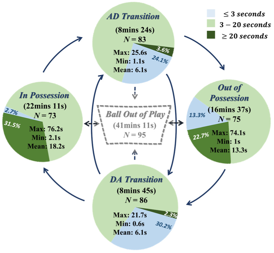
Four match phases, as well as corresponding counts, cumulative time, the maximum, minimum, and mean phase duration. Bar charts indicate the proportion of phase duration. Edges and arrows represent phase switching.

ANOVA results revealed significant differences (p< 0.001) across all tactical variables, indicating a significant effect of match phase on team tactical behaviour (Table 2). Effect sizes (η²) were large for surface area, width, lateral stretch index, and maximum and average interpersonal distance, moderate for LpW ratio, longitudinal stretch index, and minimum interpersonal distance, and small for length.

Table 2.

Mean and SD statistics with the asymptotical F-value, p-value, effect size (η²) of tactical variables.

Tacticalvariables	In possession^a	Out ofpossession^b	Attack-to-defencetransition^c	Defence-to-attacktransition^d	F	p	η ²
	Mean ± SD
Surface area (m²)	1418.0 ± 267.5^{b c d}	911.0 ± 255.7^{a c}	1081.1 ± 268.2^{a b}	1010.5 ± 238.3^a	39.125	<0.001	0.25
Length (m)	39.4 ± 4.9^{b c d}	35.2 ± 5.8^a	36.7 ± 4.8^a	36.7 ± 5.1^a	6.235	<0.001	0.04
Width (m)	52.0 ± 7.1^{b c d}	38.7 ± 7.2^{a c}	43.5 ± 8.9^{a b}	40.7 ± 7.8^a	37.33	<0.001	0.21
LpW ratio (AU)	0.78 ± 0.15^{b c d}	0.95 ± 0.24^a	0.88 ± 0.23^a	0.94 ± 0.21^a	10.541	<0.001	0.06
Stretch indexlongitudinal (m)	11.7 ± 1.5^{b c d}	10.1 ± 1.9^a	10.8 ± 1.7^a	10.7 ± 1.9^a	9.647	<0.001	0.07
Stretch indexlateral (m)	13.5 ± 1.6^{b c d}	10.1 ± 1.7^{a c}	11.1 ± 2.2^{a b}	10.5 ± 1.9^a	45.833	<0.001	0.23
Max ID (m)	56.0 ± 6.1^{b c d}	43.8 ± 6.1^{a c}	48.3 ± 7.0^{a b}	45.9 ± 6.5^a	41.915	<0.001	0.23
Min ID (m)	6.9 ± 1.8^{b c d}	5.8 ± 2.0^a	5.7 ± 1.9^a	5.6 ± 1.8^a	7.16	<0.001	0.06
Mean ID (m)	28.6 ± 2.6^{b c d}	22.8 ± 3.2^{a c}	24.7 ± 3.2^{a b}	23.9 ± 3.0^a	46.318	<0.001	0.22

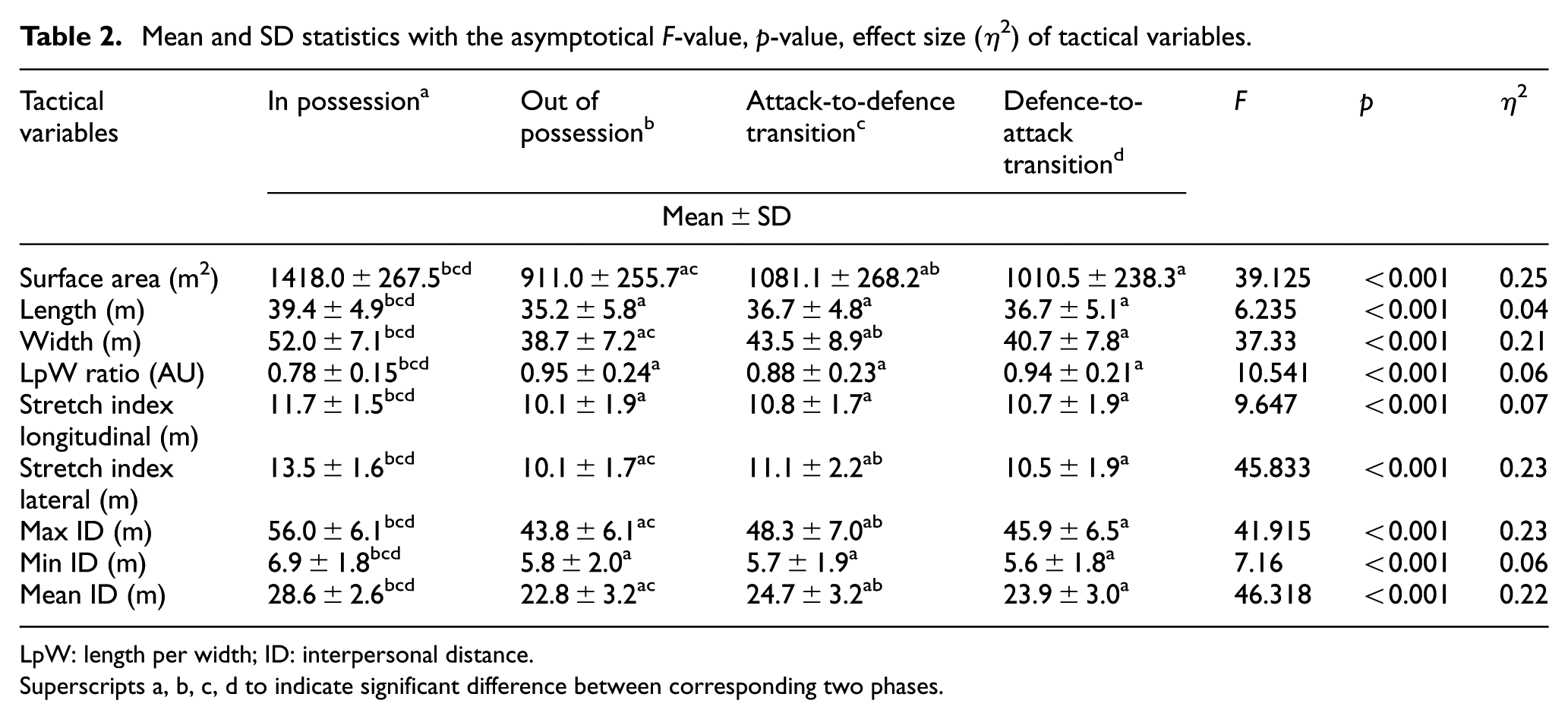
LpW: length per width; ID: interpersonal distance.

Superscripts a, b, c, d to indicate significant difference between corresponding two phases.

Pairwise comparisons revealed that team length and width during IP showed significantly greater values than the other three phases, with bigger differences in width than length (Table 2 and Figure 8). The team played with a longer and wider formation in IP than OOP (length: p < 0.001, d = 0.78; width: p < 0.001, d = 1.86), DAT (length: p < 0.01, d = 0.54; width: p< 0.001, d = 1.52), and ADT (length: p < 0.01, d = 0.54; width: p < 0.001, d = 1.05). Furthermore, the team formation was laterally elongated in IP compared to OOP (p < 0.001, d = −0.81), DAT (p < 0.001, d = −0.83), and ADT (p < 0.05, d = −0.53). The team also played wider (p < 0.01, d = 0.60) in ADT than OOP.

Figure 8.

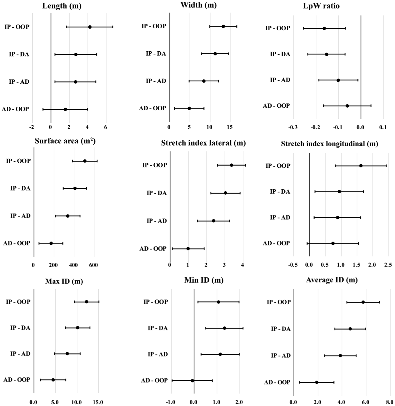
Mean differences and 95% CI of pairwise differences between phases with significant difference in tactical behaviour. Pairwise phases (OOP and DAT, DAT and ADT) without significant difference for any tactical measures were excluded.

Similar trends in team dispersion variables (surface area, lateral and longitudinal stretch indices, maximum and average ID) were found across phases. A greater area was covered in IP than OOP (p < 0.001, d = 1.94), DAT (p < 0.001, d = 1.61), ADT (p < 0.001, d = 1.25). In the lateral direction, stretch indices showed a greater magnitude in IP than OOP (p < 0.001, d = 2.0), DAT (p < 0.001, d = 1.69), ADT (p < 0.001, d = 1.23). Longer average interpersonal distance within IP was found than OOP (p < 0.001, d = 1.98), DAT (p < 0.001, d = 1.66), ADT (p < 0.001, d = 1.33). In addition, the teams showed a greater surface area (p < 0.001, d = 0.65), lateral stretch indices (p < 0.05, d = 0.51), maximum ID (p < 0.001, d = 0.68), and average ID (p < 0.01, d = 0.60) in ADT than OOP. No significant differences in tactical behaviour were found between DAT and ADT, or between DAT and OOP.

Discussion

This work aimed to establish an analytical pipeline for tactical analysis using GNSS tracking devices, which can be used with any device type (Study 1) and to demonstrate its applicability (face validation) focused on team tactical behaviour across match phases using different player tracking devices (Study 2). Positional data from GNSS tracking systems require extra data processing prior to tactical analysis, which differentiates them from optical tracking and LPM systems. While previous studies have used GNSS positional data to analyse tactical behaviour,^13–15 the lack of detailed data processing procedures has limited the reproducibility and comparability of findings. This research presented a comprehensive pipeline for processing GNSS positional data, facilitating efficient and reliable tactical analysis. This pipeline has subsequently been used to analyse tactical behaviour of a team in the competitive match across match phases as a proof of concept and face-validation.

Analytical pipeline for tactical analysis using GNSS positional data

The analytical pipeline presented various processing steps and demonstrated its applicability on independent datasets, offering solutions to potential issues prior to tactical analysis.⁴⁰ Solutions to those issues were provided in a Python script as a toolbox, including noise filtering, map projection methods, rotation matrix calculation, and data loss handling. Additionally, a comparison of two pragmatic approaches for obtaining pitch location coordinates was presented in Supplemental Documents, highlighting the trade-off between using web mapping platforms and GNSS tracking devices. Using web mapping platforms features low time cost, high consistency, and accessibility and is the recommended approach for retrieving pitch locations.

The analytical pipeline in Study 1 builds upon the analysis of Folgado et al.¹² and aids in transparent methods to analyse the complexity of team tactical performance. Additionally, the pipeline identifies missing data and proposes methods to address this issue. Although the risk of missing data should be mitigated by ensuring optimal satellite connections,⁹ the findings of Study 1 also highlight that a maximum of 0.1 s of consecutive data loss was detected. Because spatiotemporal analysis is used in Study 1, interpolation overcomes this issue that does not harm the overall analysis of team dynamics. Interpolation seems an appropriate solution when analysing “more stable” tactical patterns but might not be valid for locomotor analysis. The comprehensive approach of Study 1 will allow scientists and practitioners to expedite tactical analysis processes using GNSS tracking systems and improve the quality and reproducibility.

Tactical behaviour in competitive match play

The case study presented in Study 2 revealed insights into team tactical behaviour across match phases. Proportions of phase duration varied across match phases, with longer phases allowing players to engage more in the team’s attacking or defending behaviour. Notably, the team’s shape also varied across phases.

Previous studies showed a greater surface area and stretch index in offence than defence.^41,42 The current study further confirms significantly larger lateral stretch indices, interpersonal distances, surface area, and team width in ADT than OOP. In possession, the team length and width were greater than in other phases. Simultaneously, the team presented a rectangular shape in the lateral direction, represented by a LpW ratio lower than one. However, the team shape transitioned to a squared orientation in other phases (i.e., LPW ratio close to 1), driven by changes in team width rather than length. These findings align with previous research indicating shifts in team shapes between training and official matches⁴³ and between offensive and defensive phases.⁴² The team’s shape in official matches shifted to nearly square, compared to a more rectangular shape⁴³ in 11-a-side training games. Praça et al.⁴² reported that team shapes were almost square in offensive phases but rectangular in the lateral direction in defence.

Furthermore, the team presented a more contracted formation in OOP than ADT, suggesting a quick adaptation from offensive to defensive modes. However, a similar formation in OOP to DAT, which may imply a delayed team reaction to offensive behaviour or suggest a short period required to switch from defensive to offensive mode. In practice, these insights can inform coaches of team movements following ball recovery. Frencken et al.⁴⁴ proposed a 3-s time window for tactical analysis, based on expert football coaches’ advice on the maximal time allowed for a team to respond to game events. However, over a quarter of transition phases were found shorter than three seconds in the current analysis, which might have been overlooked if using fixed time windows. Combining event and positional data allowed us to investigate dynamic variations in team formation at each match phase. Such insights contribute to the understanding of how teams strategically adapt to different phases, offering valuable knowledge for both researchers and practitioners.

Limitations and future directions

As part of the proof-of-concept nature of the case study, some limitations should be addressed. First, while over 300 phases were analysed, the reliance on data from one match may raise concerns about the generalisability of findings. In addition, notational analysis identifying the match phases was conducted by professional analysts, introducing a level of subjectivity. Although the event data were visually inspected with video footage, this emphasises the need for data quality control and a clear definition of match phases. Furthermore, while using different device types from the same company demonstrated the applicability of the pipeline, the current pipeline has not been applied to devices from other manufacturers. To address this, a parser for checking data formats has been incorporated in the attached Python file, allowing for standardising raw data across various devices (companies).

Data loss from GNSS tracking systems is a common issue⁴⁰ and also identified in the current study. While it may not affect the primary use of GNSS tracking technology in physical monitoring, its effect on the tactical analysis needs careful consideration. The volume and frequency of data loss should be reported in future studies and require a consensus on acceptable level of positional data loss by researchers,⁴⁵ facilitating cross-study comparison. Additionally, there has yet to be a shared agreement on the optimal filter for football tactical analysis using GNSS positional data. Further research is also needed to study how different filters impact tactical analysis results. Therefore, two data-smoothing options previously used by practitioners³⁰ and scientists¹² are included in the current study for users’ convenience.

Synchronisation of positional data with event data is a crucial step but is scarcely reported in previous studies. Human error from notational analysis and systematic offset of player tracking technology and camera can introduce time lag between two data sources.¹¹ Manual synchronisation is sensible for limited sample size, but not pragmatic for large number of datasets. A solution for this was proposed by Kwiatkowski and Clark⁴⁶ using a Needlemann-Wunsch-Algorithm and can be used via packages such as sync.soccer or DataBallPy. Synchronisation is similarly important for physical analysis that is analysed across match phases, but is often not reported.⁴⁵ Standardising acceptable level of time lag for tactical or physical analysis in football is recommended to ensure data quality and the reliability of findings, facilitating comparison across studies.

Conclusions

This work provides an analytical pipeline for processing GNSS positional data and offers valuable insights into team tactical behaviour across match phases. The presented analytical pipeline was demonstrated to be applicable for analysing team tactical behaviour in match and training scenarios. The proof-of-concept revealed significant variation in team shape, dispersion, and coordination, emphasising the dynamic nature of teams’ strategic adaptation during possession. While the research provides valuable insights into team behaviour, the importance of standardised approaches and consideration of potential data loss require attention. The current pipeline contributes to the advancement and transparency of tactical analysis in sport science and holds implications for researchers and practitioners seeking a further understanding of team collective behaviour during match-play.

Supplemental Material

sj-docx-1-pip-10.1177_17543371251392456 – Supplemental material for Navigating team tactical analysis in football: An analytical pipeline leveraging player tracking technology

Supplemental material, sj-docx-1-pip-10.1177_17543371251392456 for Navigating team tactical analysis in football: An analytical pipeline leveraging player tracking technology by Guangze Zhang, Matthias Kempe, Allistair McRobert, Hugo Folgado and Sigrid B. H. Olthof in Proceedings of the Institution of Mechanical Engineers, Part P: Journal of Sports Engineering and Technology

Footnotes

Acknowledgements

The authors would like to thank the participating clubs for their data sharing.

ORCID iDs

Guangze Zhang

Hugo Folgado

Sigrid B. H. Olthof

Author contributions

All authors made substantial contributions to the manuscript. GZ, SO, MK, AM conceived the study idea and designed the analytical framework. GZ developed and implemented the analytical pipeline for data processing, with technical review and validation by MK. GZ, SO, MK, and AM contributed to the drafting of the manuscript. HF provided methodological guidance. All authors critically revised and approved the final manuscript.

Funding

The authors received no financial support for the research, authorship, and/or publication of this article.

Declaration of conflicting interests

The authors declared no potential conflicts of interest with respect to the research, authorship, and/or publication of this article.

Data availability statement

The dataset used in study 1 has been made available in the online repository (). The dataset used in study 2 cannot be shared since there is no permission from the team owning the data. Customised Python files for the analytical pipeline is also accessible in the online repository. Guidelines for using these codes have been detailed in the manuscript.

Supplemental material

Supplemental material for this article is available online.

References

Goes

Meerhoff

Bueno

MJO

, et al. Unlocking the potential of big data to support tactical performance analysis in professional soccer: a systematic review. Eur J Sport Sci 2020; 21: 481–496.

Low

Coutinho

Goncalves

, et al. A systematic review of collective tactical behaviours in football using positional data. Sports Med 2020; 50: 343–385.

Torres-Ronda

Clubb

Beanland

Tracking systems in team sports: back to basics. Sport Perform Sci Rep 2022; 8: 15.

Díez

Lozano

Arjol-Serrano

, et al. Influence of contextual factors on physical demands and technical-tactical actions regarding playing position in professional soccer players. BMC Sports Sci Med Rehabil 2021; 13: 157.

Raabe

Biermann

Bassek

, et al. Floodlight: a high-level, data-driven sports analytics framework. arXiv preprint arXiv:220602562 2022.

PySport. Kloppy: standardizing soccer tracking and event data, https://kloppy.pysport.org/ (2020, accessed 31 Dec 2024).

Oonk

DataBallPy, https://databallpy.readthedocs.io/en/latest/ (2024, accessed 1 Feb 2025).

Jackson

Polglaze

Dawson

, et al. Comparing global positioning system and global navigation satellite system measures of team-sport movements. Int J Sports Physiol Perform 2018; 13: 1005–1010.

Shergill

Twist

Highton

Importance of GNSS data quality assessment with novel control criteria in professional soccer match-play. Int J Perform Anal Sport 2021; 21: 820–830.

10.

Bao

Chang

Zhang

, et al. Filling missing values of multi-station GNSS coordinate time series based on matrix completion. Measurement 2021; 183: 109862.

11.

Anzer

Bauer

A goal scoring probability model for shots based on synchronized positional and event data in football (soccer). Front Sports Act Living 2021; 3: 624475.

12.

Folgado

Duarte

Fernandes

, et al. Competing with lower level opponents decreases intra-team movement synchronization and time-motion demands during pre-season soccer matches. PLoS ONE 2014; 9: e97145.

13.

Sampaio

Lago

Goncalves

, et al. Effects of pacing, status and unbalance in time motion variables, heart rate and tactical behaviour when playing 5-a-side football small-sided games. J Sci Med Sport 2014; 17: 229–233.

14.

Goncalves

Coutinho

Santos

, et al. Exploring team passing networks and player movement dynamics in youth association football. PLoS ONE 2017; 12: e0171156.

15.

Baptista

Travassos

Goncalves

, et al. Exploring the effects of playing formations on tactical behavior and external workload during football small-sided games. J Strength Cond Res 2020; 34: 2024–2030.

16.

Carling

Williams

Reilly

Handbook of soccer match analysis a systematic approach to improving performance. London: Routledge, 2005.

17.

Garganta

Trends of tactical performance analysis in team sports: bridging the gap between research, training and competition. Rev Port Cien Desp 2009; 9: 81–89.

18.

Grunz

Memmert

Perl

Tactical pattern recognition in soccer games by means of special self-organizing maps. Hum Mov Sci 2012; 31: 334–343.

19.

Sampaio

Macas

Measuring tactical behaviour in football. Int J Sports Med 2012; 33: 395–401.

20.

Duarte

Araujo

Freire

, et al. Intra- and inter-group coordination patterns reveal collective behaviors of football players near the scoring zone. Hum Mov Sci 2012; 31: 1639–1651.

21.

Memmert

Lemmink

KAPM

Sampaio

Current approaches to tactical performance analyses in soccer using position data. Sports Med 2016; 47: 1–10.

22.

Coito

Davids

Folgado

, et al. Capturing and quantifying tactical behaviors in small-sided and conditioned games in soccer: a systematic review. Research Quarterly for Exercise and Sport 2020; 93: 189–203.

23.

Weisstein

. Lambert conformal conic projection. MathWorld—a wolfram web resource. Champaign: Wolfram MathWorld, 2009.

24.

Rod Deakin

M. N. Hunter

Karney

The Gauss–Kruger projection. In: Victorian regional survey conference, Warrnambool: Surveyors Australia, September 10-12, 2010.

25.

Karney

CF.

Transverse Mercator with an accuracy of a few nanometers. J Geodesy 2011; 85: 475–485.

26.

Rhind

Current shortcomings of global mapping and the creation of a new geographical framework for the world. Geograph J 2000; 166: 295–305.

27.

ISCM. Commonly used map projections, https://www.icsm.gov.au/education/fundamentals-mapping/projections/commonly-used-map-projections (2020, accessed 17 Oct 2024).

28.

Castellano

Fernández

Echeazarra

, et al. Influence of pitch length on inter- and intra-team behaviors in youth soccer. An Psicol 2017; 33: 486–496.

29.

Steffensen

JF.

Interpolation. New York: Mineola NY, 2006.

30.

Shaw

LaurieOnTracking, https://github.com/Friends-of-Tracking-Data-FoTD/LaurieOnTracking (2021, accessed 01 May 2022).

31.

Zanin

Azzalini

Ranaweera

, et al. Designing a small-sided game to elicit attacking tactical behaviour in professional rugby union forwards. J Sports Sci 2022; 40: 2304–2314.

32.

Hudl. Hudl Sportscode, https://www.hudl.com/products/sportscode (2007, accessed 23 June 2025).

33.

O’Donoghue

An introduction to performance analysis of sport. London: Routledge, 2015.

34.

OPTAStatsPerform. Opta Event Definitions, https://www.statsperform.com/opta-event-definitions/ (2025, accessed 17 July 2025).

35.

Olthof

SBH

Frencken

WGP

Lemmink

. A match-derived relative pitch area facilitates the tactical representativeness of small-sided games for the official soccer match. J Strength Cond Res 2019; 33: 523–530.

36.

Frencken

Lemmink

Delleman

, et al. Oscillations of centroid position and surface area of soccer teams in small-sided games. Eur J Sport Sci 2011; 11: 215–223.

37.

Olthof

Frencken

Lemmink

KA.

The older, the wider: on-field tactical behavior of elite-standard youth soccer players in small-sided games. Hum Mov Sci 2015; 41: 92–102.

38.

Cohen

Statistical power analysis for the behavioral sciences. 2nd ed. New York, NY: Routledge, 1988.

39.

Field

Discovering statistics using IBM SPSS statistics. Los Angeles, London, New Delhi: Sage, 2013.

40.

Capaccio

Lowe

Walsh

DMA

, et al. Real-time differential GPS/GLONASS trials in Europe using all-in-view 20-channel receivers. J Navig 1997; 50: 193–208.

41.

Clemente

Couceiro

Martins

, et al. Measuring tactical behaviour using technological metrics: case study of a football game. Int J Sports Sci Coach 2013; 8: 723–739.

42.

Praça

Moreira

PED

de Andrade

AGP

, et al. Integrating notational and positional analysis to investigate tactical behavior in offensive and defensive phases of football matches. Proc IMechE, Part P: J Sports Engineering and Technology 2022; 239(2): 264–273.

43.

Olthof

SBH

Frencken

WGP

Lemmink

. When something is at stake: differences in soccer performance in 11 vs. 11 during official matches and training games. J Strength Cond Res 2019; 33: 167–173.

44.

Frencken

Van Der Plaats

Visscher

, et al. Size matters: pitch dimensions constrain interactive team behaviour in soccer. J Syst Sci Complex 2013; 26: 85–93.

45.

Doran

Hawkins

, et al. Contextualised peak periods of play in English Premier League matches. Biol Sport 2022; 39(4): 973–983.

46.

Kwiatkowski

Clark

The right way to synchronise event and tracking data, https://kwiatkowski.io/sync.soccer (2020, accessed 1 Mar 2025).

Supplementary Material

Please find the following supplemental material available below.

For Open Access articles published under a Creative Commons License, all supplemental material carries the same license as the article it is associated with.

For non-Open Access articles published, all supplemental material carries a non-exclusive license, and permission requests for re-use of supplemental material or any part of supplemental material shall be sent directly to the copyright owner as specified in the copyright notice associated with the article.

0.00 MB

3.05 MB