Sage Journals: Discover world-class research

Abstract

Determining the players’ playing styles and bringing the right players together are very important for winning in basketball. This study aimed to group basketball players into similar clusters according to their playing styles for each of the traditionally defined five positions (point guard (PG), shooting guard (SG), small forward (SF), power forward (PF), and center (C)). This way, teams would be able to identify their type of players to help them determine what type of players they should recruit to build a better team. The 17 game-related statistics from 15 seasons of the National Basketball Association (NBA) were analyzed using a hierarchical clustering method. The cluster validity indices (CVIs) were used to determine the optimum number of groups. Based on this analysis, four clusters were identified for PG, SG, and SF positions, while five clusters for PF position and six clusters for C position were established. In addition to the definition of the created clusters, their individual achievements were examined based on three performance indicators: adjusted plus-minus (APM), average points differential, and the percentage of clusters on winning teams. This study contributes to the evaluation of team compatibility, which is a significant part of winning, as it allows one to determine the playing styles for each position, while examining the success of position pair combinations.

Keywords

Sport analytics performance analysis basketball positions clustering cluster validity indices

Introduction

All over the world, sports have received increased attention over the past few decades. Naturally, the sports industry has also generated great value and revenue. Basketball is one of the most popular and watched sports globally, and the National Basketball Association (NBA) is the most prominent organization in this sport. In the NBA, it is crucial to be successful during the season and advance to the playoffs because playoff participation is strongly relevant to team valuation and annual total revenue.¹ With the rapidly increasing data volume, new methods, and technologies for their analysis, sports analytics is an emerging area where teams receive support for this success. As a scientific field, sports analytics deals with the historical and real-time data collection and analysis about sports in general.² In basketball, where the winner is so important, many studies try to determine the performance indicators that best distinguish the winner and the loser.^3–11 In some of these studies, the match’s location was also taken into account.^12,13 Besides these, other studies examined different parameters, such as starter and nonstarter players.^14–18 Lastly, some studies determined the stats affecting winning for different stages of the tournament.^19–22

Since it is one of the most critical factors of the game, many studies have evaluated player performances. Metrics such as Player Efficiency Rating (PER), Performance Index Rating (PIR), Plus Minus (+/−), which give an overall score to the players, are widely used.^23,24 In addition to these metrics, operational research methods used in many fields of sports (tactics and strategy, scheduling, and forecasting) were also used in player performance assessment.²⁵ When the related literature was analyzed, multi-criteria decision-making methods were widely used to find the best player.^26–29 Data envelopment analysis was one of the most preferred techniques.^30–33

In these performance evaluation studies, the playing positions of the players were generally not taken into account. Since basketball is a game played with five players on the court, the players are traditionally listed under five different groups (i.e. point guard (PG), shooting guard (SG), small forward (SF), power forward (PF), and center (C)). These groups represent player positions and describe the role of players on a team. Some studies analyzed position performance from different perspectives.^34–37 However, the evolution of the game has made these traditional positions inadequate for modern basketball. With this evolution, players develop themselves and create differences in their games. Thus, players who can play in different positions or have different game styles despite playing in the same position have emerged.³⁸ Considering that these positions provide a framework for coaches to build a team, the deficiency becomes even more prominent. As in this study, a number of studies were carried out to regroup the players to address this issue.

In two of these previous studies, the players were grouped according to factors other than game-related statistics. While Zhang et al.³⁹ used the anthropometric attributes and the playing experience of players, Mateus et al.⁴⁰ investigated the player-related and contextual variables to group basketball players. Both of them applied a two-step cluster analysis with log-likelihood as the distance measure and Schwartz’s Bayesian criterion. Then, the created clusters were analyzed according to the game-related statistics. There have also been studies that directly use box-score data for clustering. Zhang et al.⁴¹ regrouped only the guards who played in the 2014/2015 NBA season. They preferred to use the k-means method for cluster analysis. Bianchi et al.⁴² also used the k-means method in their research. They clustered the 476 players based on only the seven game stats from the 2010/2011 NBA season. In another study, Patel⁴³ used the box-score data, and applied the k-means method. In this study, 18 game stats from the 2016/2017 NBA season were used. Diambra⁴⁴ also used the box-score data for cluster analysis. Both Patel and Diambra applied the Principal Component Analysis (PCA) technique to reduce the dimensionality of the game stats.

Although the box-score data are widely used, it is not considered reliable in identifying players because confounding factors like team pace and playing times often lead to confusion. For example, consider two players who get the same number of rebounds, but play on two different teams. Their rebounding ability cannot be equal, even if they get equal playing time, because the number of available rebounds depends on the number of missed shots. Therefore, when examining the ability of players to get rebounds, the rates in advanced stats, which also count on all available rebounds, stand out. As another example, players playing on two different teams and making the same number of turnovers cannot be interpreted as having the same ball-handling abilities. The ratio of how many turnovers these players make versus how many balls they use is more reliable than the number of turnovers in determining their ball-handling abilities. Advanced statistics like rates and efficiency metrics were used in some studies to eliminate this confusion and obtain reliable results. Lutz⁴⁵ analyzed 329 players who played in the 2010/2011 NBA regular season. In addition to advanced statistics, he also included shooting statistics in his research and used an expectation-maximization (EM) algorithm as a method for clustering. In the same year, Alagappan⁴⁶ applied the Topological Data Analysis (TDA) method, which was used to identify cancer cells. With this work, Alagappan received the best research award at the MIT Sloan Sports Analytics Conference, the biggest conference in the sports analytics area. Kalman and Bosch⁴⁷ presented their research at the same conference in 2020. As in Lutz’s work, they also used EM algorithms and added shooting statistics in their variables.

The main purpose of this study was to group basketball players into similar clusters for each of the five positions. Previous studies have contributed to the literature by regrouping players according to their playing style. However, these studies overlook the fact that even if classical positions are insufficient, they are useful in practice because basketball is played with five players on the court. Therefore, unlike the existing literature, in this study, instead of suggesting new positions for basketball, players were classified into existing positions. Hence, this study supports coaches in defining the play styles of their players for each position. Coaches would be able to decide more easily what type of player they should consider for the missing position with the guidance of this study, which provides the success of a two-player combination. The research design of this study is illustrated in Figure 1.

Figure 1.

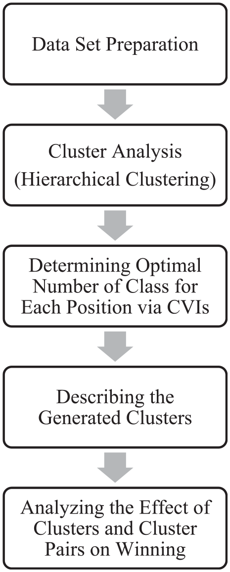
Illustration of research design.

Methods

In this section, the data set preparation is briefly described, and the procedure of the cluster analysis is summarized. The basketball-reference.com website,⁴⁸ in which a wide range of free basketball data is offered, especially for the years following the 2000/2001 NBA season, was used as a data source. The variables were selected considering they accurately reflect the playing styles of players. The explanations are included and the data analyses were performed using the R programing language.⁴⁹

Sample

The data were obtained from the basketball-reference.com website, from which a wide range of free basketball data was offered, especially for the years following the 2000/2001 NBA season.⁴⁸ For this analysis, data were evaluated from the 2000/2001 season to the 2015/2016 season. However, due to the boycott in the NBA in the 2011/2012 season, fewer matches were played than the regular season. For this reason, it was decided to eliminate the data for the 2011/2012 season and prepare a data set with 15 seasons of data (2000/2001 to 2015/2016, except 2011/2012).

Considering that a five-man lineup analysis will be conducted in the future phase of this study, some restrictions were implemented to improve data reliability. It was decided that the five players to be evaluated must have played together in at least 21 matches and should have had a minimum of 240 min in total playing time. After those limitations, 565 five-man lineups matching the criteria for the 15 seasons were found.

The players’ data were collected from multiple tables⁴⁸ and joined together on the player’s name, season, and team name. The total number of observations was 6040 for 72 variables. These variables were a combination of advanced statistics, shot distribution statistics, and play-by-play stats. Once created, the dataset was cleared by removing duplicate columns, columns that were not considered to contribute to the work, and columns with null values. As indicated on their website, basketball-reference.com makes great efforts to provide accurate information. To validate the advanced statistics provided by the data source, randomly selected player stats were obtained from the official NBA website (www.nba.com/stats),⁵⁰ and advanced statistics were calculated with the formulas given in Table 1. The calculated advanced stats matched the data provided by basketball-reference.com.

Table 1.

The names and descriptions of the selected advanced statistics.⁵¹

Advanced stats
Abbreviations	Names	Descriptions
PER	Player efficiency rating	This statistic, developed by John Hollinger, calculates the productivity of the player per minute. In general, PER collects the player’s positive statistics, then extracts the negative statistics.
TS%	True shooting percentage	This statistic shows the shooting efficiency, unlike the field goal percentage which considers field goals, three-point field goals, and free throws. The formula is; PTS/(2 × (FGA + 0.44 × FTA)).
3PAr	Three-point attempt rate	It is a statistic showing the rate of shots the player made from the three-point range.
FTr	Free throw attempt rate	It is a rate of going to the foul line against field goal attempts.
ORB%	Offensive rebound percentage	It is a percentage of a player getting available offensive rebounds when he is on the floor. The formula is 100 × (ORB × (Tm MP/5))/(MP × (Tm ORB + Opp DRB)).
DRB%	Defensive rebound percentage	It is a percentage of a player getting available defensive rebounds when he is on the floor. The formula is 100 × (DRB × (Tm MP/5))/(MP × (Tm DRB + Opp ORB)).
AST%	Assist percentage	It is a percentage of teammate field goals a player assisted with while he is on the floor. The formula is 100 × AST/(((MP/(Tm MP/5)) × Tm FGM) − FGM).
STL%	Steal percentage	It is a percentage of opponent possessions that end with a steal by the player while he is on the floor. The formula is 100 × (STL × (Tm MP/5))/(MP × Opp Poss).
BLK%	Block percentage	It is a percentage of opponent two-point field goal attempts blocked by the player while he is on the floor. The formula is 100 × (BLK × (Tm MP/5))/(MP × (Opp FGA − Opp 3PA)).
TO%	Turnover percentage	This statistic calculates the percentage of turnover per 100 plays. The formula is 100 × TOV/(FGA + 0.44 × FTA + TOV).
USG%	Usage percentage	It is a percentage of using the ball by the player while he is on the floor. The formula is 100 × ((FGA + 0.44 × FTA + TOV) × (Tm MP/5))/(MP × (Tm FGA+0.44 × Tm FTA + Tm TOV)).

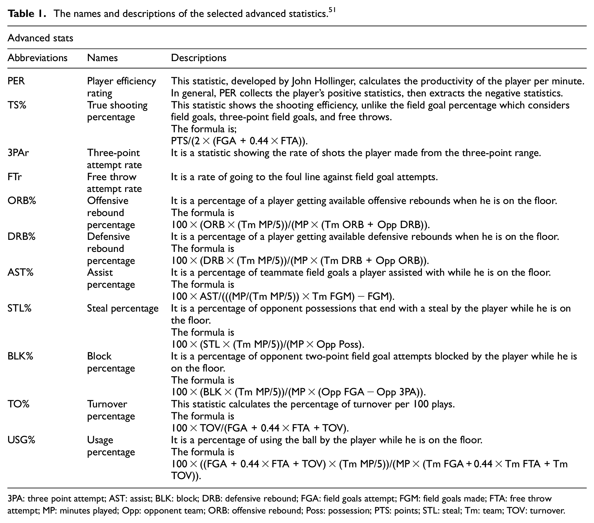
3PA: three point attempt; AST: assist; BLK: block; DRB: defensive rebound; FGA: field goals attempt; FGM: field goals made; FTA: free throw attempt; MP: minutes played; Opp: opponent team; ORB: offensive rebound; Poss: possession; PTS: points; STL: steal; Tm: team; TOV: turnover.

Realizing that players must be clustered into their positions, yet players could play in different positions, their positions had to be determined. In order to determine the position of a player, the percentage distributions of positions played by each player from the basketball-reference website were used. If the player played more than 25% in a position in a single season, it was assumed that the player could play in that position. Hence, a player could be included in the cluster of different positions in the same season. Also, the same players who played in different seasons were included in the clustering for each season, considering the possibility of seasonal changes in the players’ style of play.

The restrictions and the assumptions of this study are summarized below.

-2011/2012 NBA season statistics were excluded due to the boycott in the NBA

-The players who played less than 240 min in a single season were excluded

-The players who played less than 21 matches in a single season were excluded

-The player who played more than 25% in a position in a single season were included in that position

In this way, lists of players to be classified for five positions were created. About 426 players in the PG position, 490 players in the SG position, 544 players in the SF position, 522 players in the PF position, and 525 players in the C position took part in the cluster analyses.

Variables

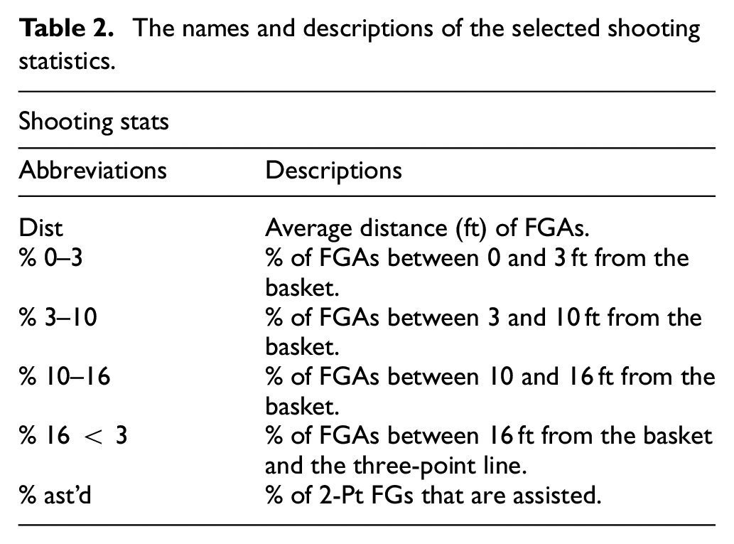
For cluster analysis, statistics were chosen so as to reflect the game styles in the best way. After examining the existing literature, 17 statistics were determined – 11 were selected from advanced statistics and 6 were shooting statistics. Advanced statistics were preferred in this study since the players’ evaluation yielded more efficient results than box-score statistics. With some calculations in advanced statistics, the factors that cause mistakes in evaluating the players are reduced (i.e. playing times, teams’ effect). For a detailed analysis of the offensive characters of the players, shooting statistics were selected. This selection aimed to determine the style of the players, rather than their success, so the shooting distance of the field goal attempts was evaluated, not the field goals made. The names and descriptions of the selected statistics are shown in Tables 1 and 2.

Table 2.

The names and descriptions of the selected shooting statistics.

Shooting stats
Abbreviations	Descriptions
Dist	Average distance (ft) of FGAs.
% 0–3	% of FGAs between 0 and 3 ft from the basket.
% 3–10	% of FGAs between 3 and 10 ft from the basket.
% 10–16	% of FGAs between 10 and 16 ft from the basket.
% 16 < 3	% of FGAs between 16 ft from the basket and the three-point line.
% ast’d	% of 2-Pt FGs that are assisted.

Procedure and data analysis

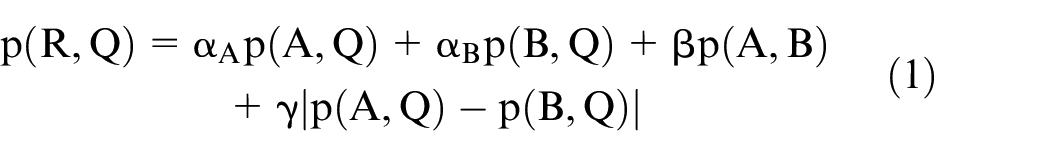
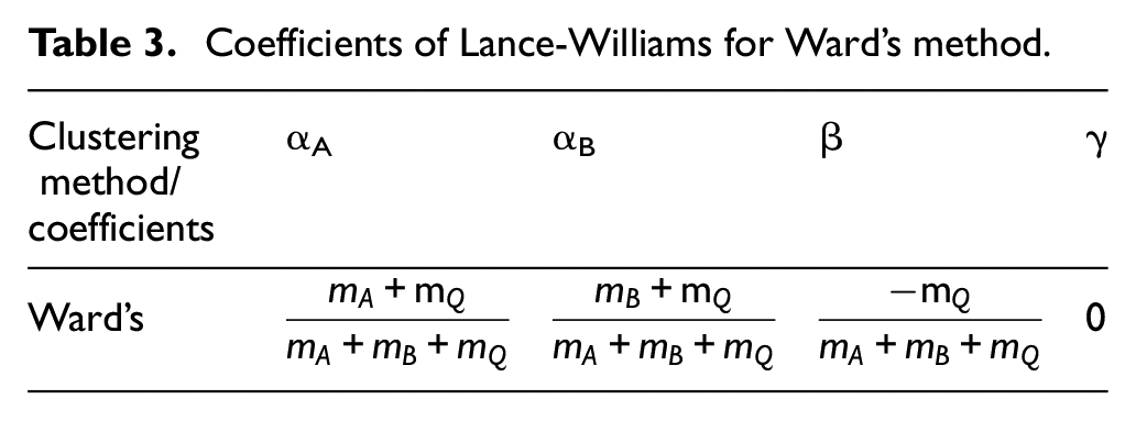
After preparing the data set, the clustering analysis was started using a Hclust function in R software. The Hclust function performs hierarchical clustering analysis with the agglomerative method. In each stage, according to the chosen method, the distance between the clusters is recalculated with the Lance-Williams similarity update formula given in equation (1). In this equation, the p (.,.) denotes the proximity function. The coefficients in the equation vary according to the chosen model, where m_A, m_B, and m_Q denote the number of dots in clusters (see Table 3). In this study, the Ward method was used. This method has been widely used after it was proposed for the first time in 1963 and gave better results in previous comparison studies, especially when the group proportions were approximately equal. The objective of the Ward method is to minimize within-cluster variance.^52–54 To achieve this, the method considers the increase in squared error after merging the clusters.⁵⁵ Ward’s criteria were added to this method in 2014, and it is in the R programing with the name of “Ward.D2.”^56,57

\begin{matrix} p (R, Q) = α_{A} p (A, Q) + α_{B} p (B, Q) + β p (A, B) \\ + γ | p (A, Q) - p (B, Q) | \end{matrix}

(1)

Table 3.

Coefficients of Lance-Williams for Ward’s method.

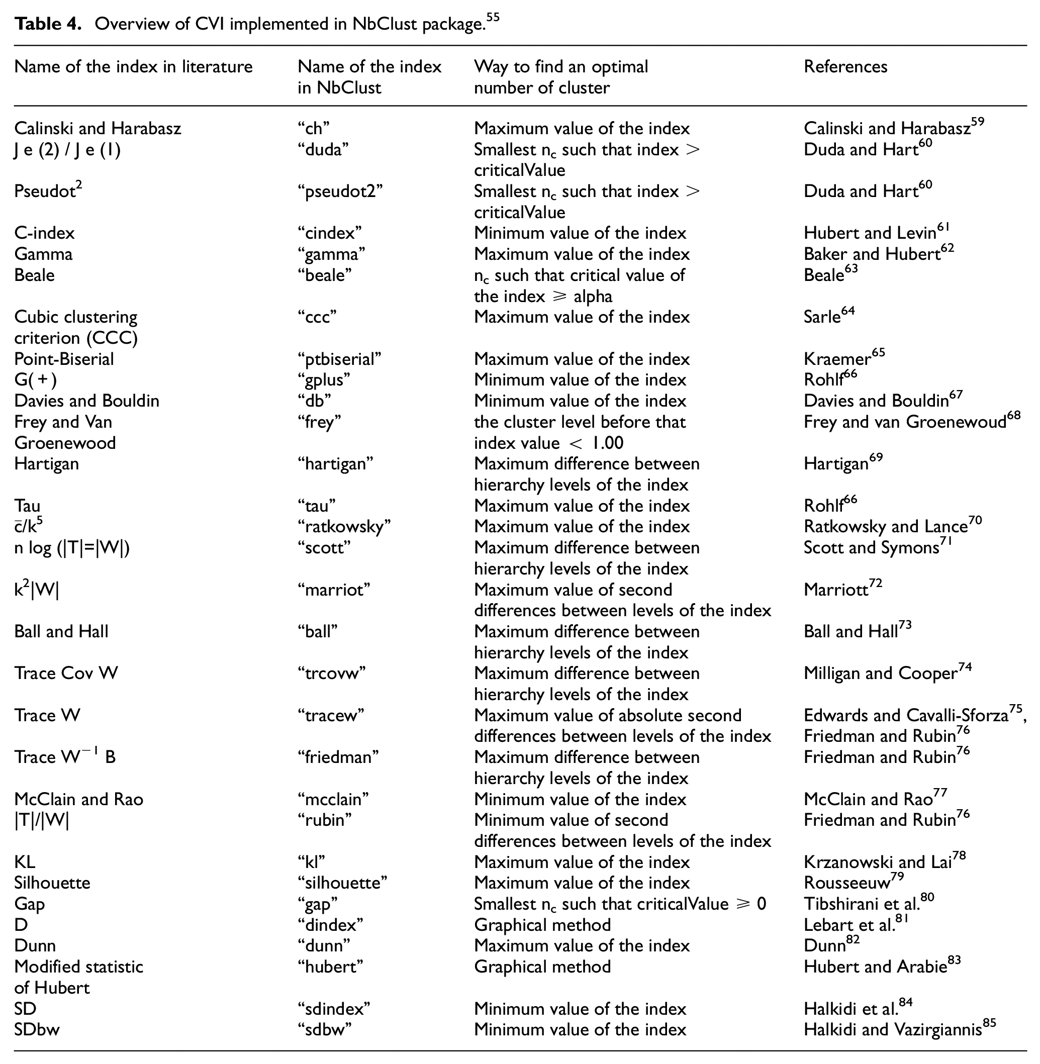
Clustering method/coefficients	α_A	α_B	β	γ
Ward’s	$\frac{m_{A} + m_{Q}}{m_{A} + m_{B} + m_{Q}}$	$\frac{m_{B} + m_{Q}}{m_{A} + m_{B} + m_{Q}}$	$\frac{- m_{Q}}{m_{A} + m_{B} + m_{Q}}$	0

For this analysis, since the number of sets was unknown in advance, the most suitable number of clusters was selected by comparing several sets. As such, cluster analysis was performed with a minimum of four and a maximum of ten groups for each position. The number of players of the resulting clusters is shown in Table A1. The majority of the methods used to determine the optimal number of clusters are based on internal validity indices. Arbelaitz et al.⁵⁸ called these indexes Cluster Validity Index (CVI) and stated no definitive conclusion about which was the best in the literature. However, Charrad et al.⁵⁵ declared two ways to determine the most appropriate number of clusters in their study. They explained that the first one is to choose according to the majority rule, that is, to choose the most chosen number of indexes, and the other way is to choose among the indexes that are found to be preponderant with previous simulation studies. In this study, clusters were formed by considering the majority rule. To see the result of the majority rule, the NbClust package, which was created by Charrad et al.⁵⁵ and had 30 CVI comparisons, was used. In addition, some of the leading indexes in the simulation studies were expected to support this result. The 30 indexes and their descriptions in this package are shown in Table 4.

Table 4.

Overview of CVI implemented in NbClust package.⁵⁵

Name of the index in literature	Name of the indexin NbClust	Way to find an optimal number of cluster	References
Calinski and Harabasz	“ch”	Maximum value of the index	Calinski and Harabasz⁵⁹
J e (2) / J e (1)	“duda”	Smallest n_c such that index > criticalValue	Duda and Hart⁶⁰
Pseudot²	“pseudot2”	Smallest n_c such that index > criticalValue	Duda and Hart⁶⁰
C-index	“cindex”	Minimum value of the index	Hubert and Levin⁶¹
Gamma	“gamma”	Maximum value of the index	Baker and Hubert⁶²
Beale	“beale”	n_c such that critical value of the index ≥ alpha	Beale⁶³
Cubic clustering criterion (CCC)	“ccc”	Maximum value of the index	Sarle⁶⁴
Point-Biserial	“ptbiserial”	Maximum value of the index	Kraemer⁶⁵
G(+)	“gplus”	Minimum value of the index	Rohlf⁶⁶
Davies and Bouldin	“db”	Minimum value of the index	Davies and Bouldin⁶⁷
Frey and Van Groenewood	“frey”	the cluster level before that index value < 1.00	Frey and van Groenewoud⁶⁸
Hartigan	“hartigan”	Maximum difference between hierarchy levels of the index	Hartigan⁶⁹
Tau	“tau”	Maximum value of the index	Rohlf⁶⁶
$\bar{c}$ /k⁵	“ratkowsky”	Maximum value of the index	Ratkowsky and Lance⁷⁰
n log (\|T\|=\|W\|)	“scott”	Maximum difference between hierarchy levels of the index	Scott and Symons⁷¹
k²\|W\|	“marriot”	Maximum value of second differences between levels of the index	Marriott⁷²
Ball and Hall	“ball”	Maximum difference between hierarchy levels of the index	Ball and Hall⁷³
Trace Cov W	“trcovw”	Maximum difference between hierarchy levels of the index	Milligan and Cooper⁷⁴
Trace W	“tracew”	Maximum value of absolute second differences between levels of the index	Edwards and Cavalli-Sforza⁷⁵, Friedman and Rubin⁷⁶
Trace W⁻¹ B	“friedman”	Maximum difference between hierarchy levels of the index	Friedman and Rubin⁷⁶
McClain and Rao	“mcclain”	Minimum value of the index	McClain and Rao⁷⁷
\|T\|/\|W\|	“rubin”	Minimum value of second differences between levels of the index	Friedman and Rubin⁷⁶
KL	“kl”	Maximum value of the index	Krzanowski and Lai⁷⁸
Silhouette	“silhouette”	Maximum value of the index	Rousseeuw⁷⁹
Gap	“gap”	Smallest n_c such that criticalValue ≥ 0	Tibshirani et al.⁸⁰
D	“dindex”	Graphical method	Lebart et al.⁸¹
Dunn	“dunn”	Maximum value of the index	Dunn⁸²
Modified statistic of Hubert	“hubert”	Graphical method	Hubert and Arabie⁸³
SD	“sdindex”	Minimum value of the index	Halkidi et al.⁸⁴
SDbw	“sdbw”	Minimum value of the index	Halkidi and Vazirgiannis⁸⁵

In summary, the steps of the applied cluster analysis are as follows:

Step 1: Players were divided into different groups from four to ten players for each position via hierarchical clustering

Step 2: Hclust function in R software was used, and Ward method was chosen for clustering

Step 3: The optimum number of clusters was determined based on CVIs

Step 4: The 30 CVIs were compared via the NbClust package in R software

Step 5: Along with the majority rule, the number of clusters was clarified with the CVI confirmation, which stands out in the simulation studies in the literature.

Results

As a result of the analysis conducted using the NbClust package, the cluster numbers for each position were determined according to the majority rule, as shown in Table 5. When looking at simulation studies in the literature, it was noticed that the research by Milligan and Cooper⁷⁴ is one of the most cited studies. More recently, Arbelaitz et al.⁵⁸ had a study comparing 30 indexes. These studies indicated that the Silhouette index was more successful compared to other CVI. After the literature review, it was observed that other studies also support this result.^86–89 As seen in Table 5, the result of the Silhouette index also supports the number of clusters determined by the majority rule in this study. Hence, four clusters for PG, SG, and SF positions, five clusters for PF position, and six clusters for C position were generated. Figure 2 shows the distribution of the players among clusters for each position, and dendrogram images of the created groups are shown in the Appendix (see Figures A1 –A5).

Table 5.

Comparison of CVI results.

	Index in NbClust	Optimal number of clusters for
		PG	SG	SF	PF	C
1	KL	4	7	4	4	4
2	CH	4	4	4	4	4
3	Hartigan	10	6	8	5	6
4	CCC	4	6	4	4	10
5	Scott	6	5	6	5	5
6	Marriot	6	7	6	5	5
7	TrCoVW	5	6	5	5	6
8	Tracew	6	6	7	5	6
9	Friedman	5	6	5	5	5
10	Rubin	6	6	8	5	6
11	Cindex	9	8	4	8	7
12	DB	10	10	10	5	7
13	Silhouette	4	4	4	5	6
14	Duda	4	9		7	7
15	Pseudot2	4	9		7	7
16	Beale	4			7	8
17	Ratkowsky	4	4	4	4	4
18	Ball	5	5	5	5	5
19	PtBiserial	4	4	4	5	6
20	GAP	4	4	4	4	4
21	Frey	4
22	McClain	4	4	4	4	4
23	gamma	10	10	10	9	10
24	gplus	10	10	10	10	10
25	tau	4	6		10	10
26	Dunn	10	9	6	9	8
27	Hubert	6				7
28	Sdindex	10	4	4	4	7
29	Dindex
30	SDbw	10	10	10	5	10
	Majority rule	4	4	4	5	6

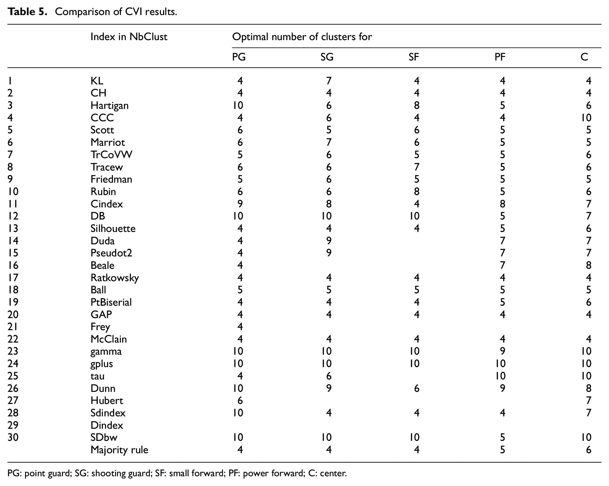
PG: point guard; SG: shooting guard; SF: small forward; PF: power forward; C: center.

Figure 2.

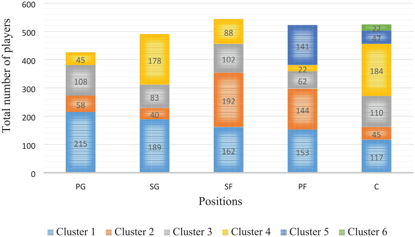
Distribution of the players among clusters for each position. (In each bar, clusters are arranged from bottom to top as Cluster 1–Cluster 6, respectively; PG: point guard; SG: shooting guard; SF: small forward; PF: power forward; C: center).

By looking at the z scores of clusters for each variable, statistics above or below the mean were observed. Then the groups were labeled according to these statistics showing their differences from each other. For example, in the PG position, Dist and 3PAr statistics of the PG3 group were above the average, while FTr and %FGA3-10 statistics of the PG3 group appeared below the average. In these prominent statistics, it is understood that this group of players shoots from long distances more than the other groups, attacked to the rim less, and went less to the free-throw line. In line with this information, the name of the “Shooter” was deemed appropriate for this group. However, it should not be overlooked that these denominations are purely for general information purposes and the group of players is more important than the groups’ name. The clusters formed within each position were named according to the prominent statistics. In the following section, along with a brief description, tables containing the cluster information (names, numbers, the superior and inferior statistics, and example players) are given (see Tables 6 –10). In addition, their means and standard deviations are given in the Appendix to describe created clusters (see Tables A2 –A6). Whether the means differ between clusters was also examined using a line chart (see Figures A6 –A10). The graphs show the z scores of the clusters for each variable. The fact that clusters have a unique line emphasizes that the means of clusters differ for each variable. Thus, these graphs helped show that the selected statistics were appropriate and the created clusters were separate.

Table 6.

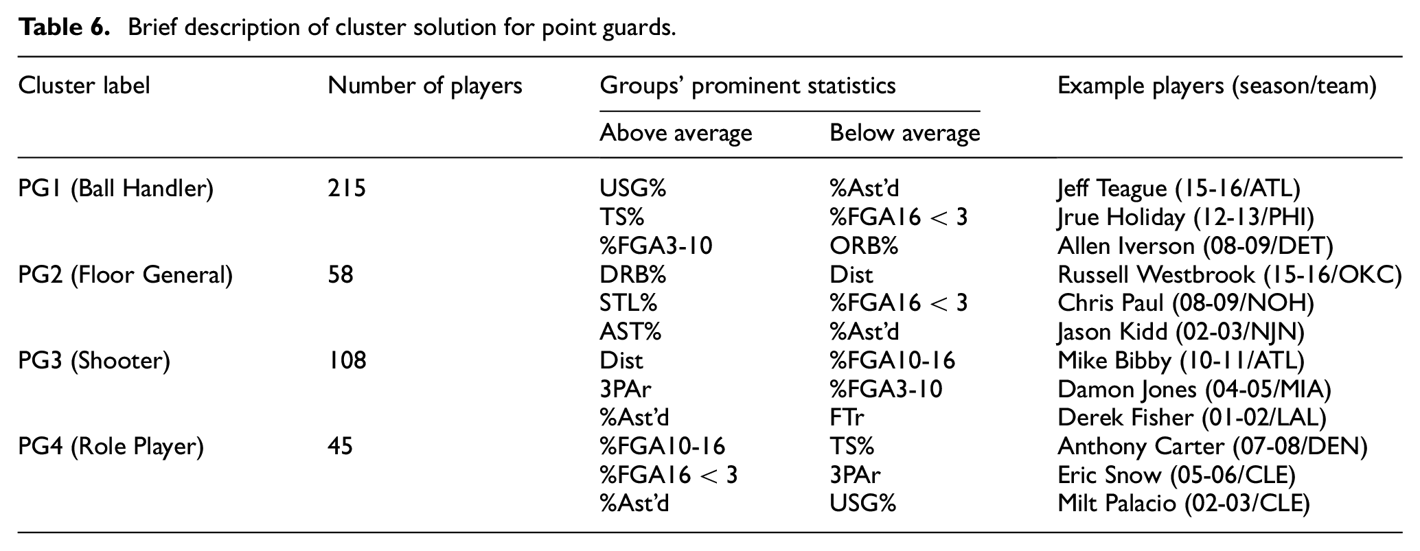
Brief description of cluster solution for point guards.

Cluster label	Number of players	Groups’ prominent statistics		Example players (season/team)
Cluster label	Number of players	Above average	Below average	Example players (season/team)
PG1 (Ball Handler)	215	USG%	%Ast’d	Jeff Teague (15-16/ATL)
		TS%	%FGA16<3	Jrue Holiday (12-13/PHI)
		%FGA3-10	ORB%	Allen Iverson (08-09/DET)
PG2 (Floor General)	58	DRB%	Dist	Russell Westbrook (15-16/OKC)
		STL%	%FGA16<3	Chris Paul (08-09/NOH)
		AST%	%Ast’d	Jason Kidd (02-03/NJN)
PG3 (Shooter)	108	Dist	%FGA10-16	Mike Bibby (10-11/ATL)
		3PAr	%FGA3-10	Damon Jones (04-05/MIA)
		%Ast’d	FTr	Derek Fisher (01-02/LAL)
PG4 (Role Player)	45	%FGA10-16	TS%	Anthony Carter (07-08/DEN)
		%FGA16<3	3PAr	Eric Snow (05-06/CLE)
		%Ast’d	USG%	Milt Palacio (02-03/CLE)

Table 7.

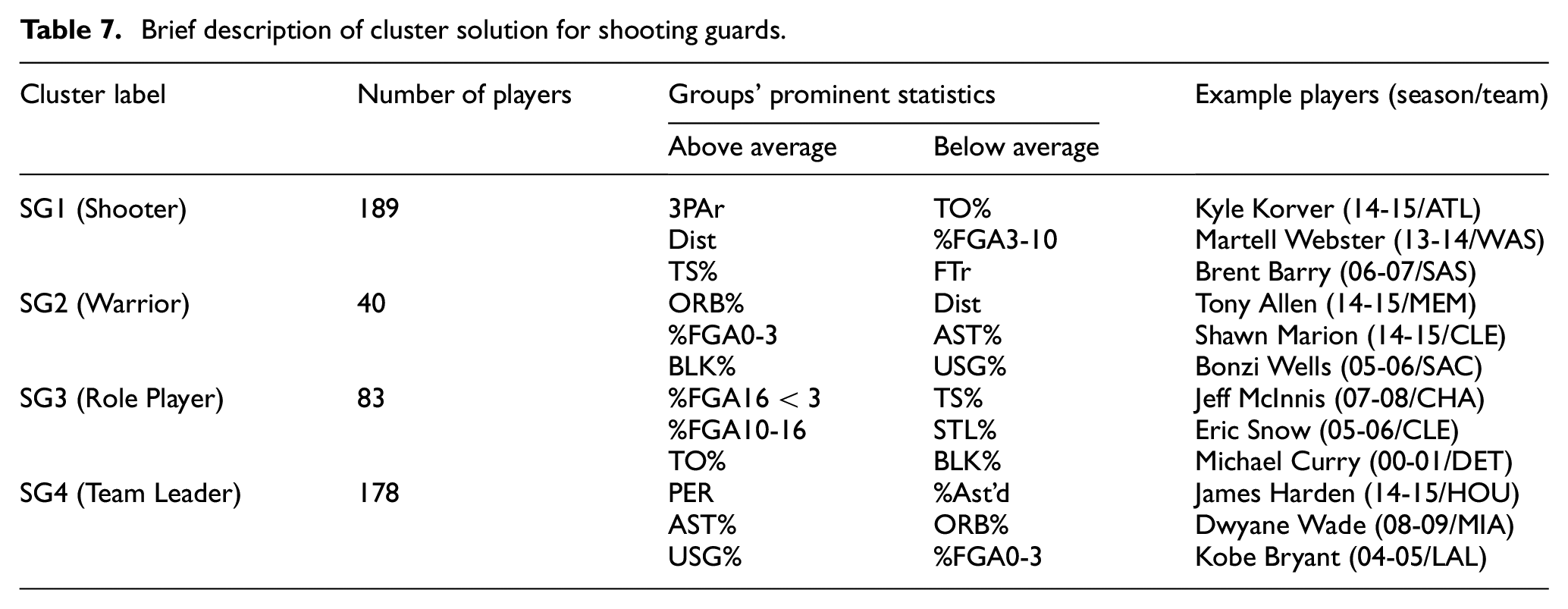
Brief description of cluster solution for shooting guards.

Cluster label	Number of players	Groups’ prominent statistics		Example players (season/team)
Cluster label	Number of players	Above average	Below average	Example players (season/team)
SG1 (Shooter)	189	3PAr	TO%	Kyle Korver (14-15/ATL)
		Dist	%FGA3-10	Martell Webster (13-14/WAS)
		TS%	FTr	Brent Barry (06-07/SAS)
SG2 (Warrior)	40	ORB%	Dist	Tony Allen (14-15/MEM)
		%FGA0-3	AST%	Shawn Marion (14-15/CLE)
		BLK%	USG%	Bonzi Wells (05-06/SAC)
SG3 (Role Player)	83	%FGA16<3	TS%	Jeff McInnis (07-08/CHA)
		%FGA10-16	STL%	Eric Snow (05-06/CLE)
		TO%	BLK%	Michael Curry (00-01/DET)
SG4 (Team Leader)	178	PER	%Ast’d	James Harden (14-15/HOU)
		AST%	ORB%	Dwyane Wade (08-09/MIA)
		USG%	%FGA0-3	Kobe Bryant (04-05/LAL)

Table 8.

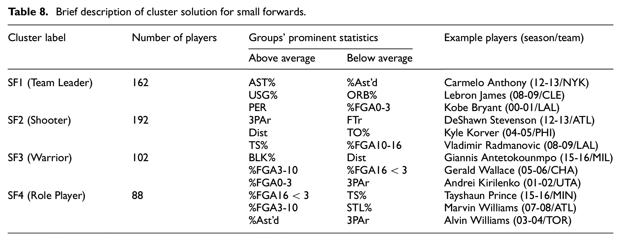
Brief description of cluster solution for small forwards.

Cluster label	Number of players	Groups’ prominent statistics		Example players (season/team)
Cluster label	Number of players	Above average	Below average	Example players (season/team)
SF1 (Team Leader)	162	AST%	%Ast’d	Carmelo Anthony (12-13/NYK)
		USG%	ORB%	Lebron James (08-09/CLE)
		PER	%FGA0-3	Kobe Bryant (00-01/LAL)
SF2 (Shooter)	192	3PAr	FTr	DeShawn Stevenson (12-13/ATL)
		Dist	TO%	Kyle Korver (04-05/PHI)
		TS%	%FGA10-16	Vladimir Radmanovic (08-09/LAL)
SF3 (Warrior)	102	BLK%	Dist	Giannis Antetokounmpo (15-16/MIL)
		%FGA3-10	%FGA16<3	Gerald Wallace (05-06/CHA)
		%FGA0-3	3PAr	Andrei Kirilenko (01-02/UTA)
SF4 (Role Player)	88	%FGA16<3	TS%	Tayshaun Prince (15-16/MIN)
		%FGA3-10	STL%	Marvin Williams (07-08/ATL)
		%Ast’d	3PAr	Alvin Williams (03-04/TOR)

Table 9.

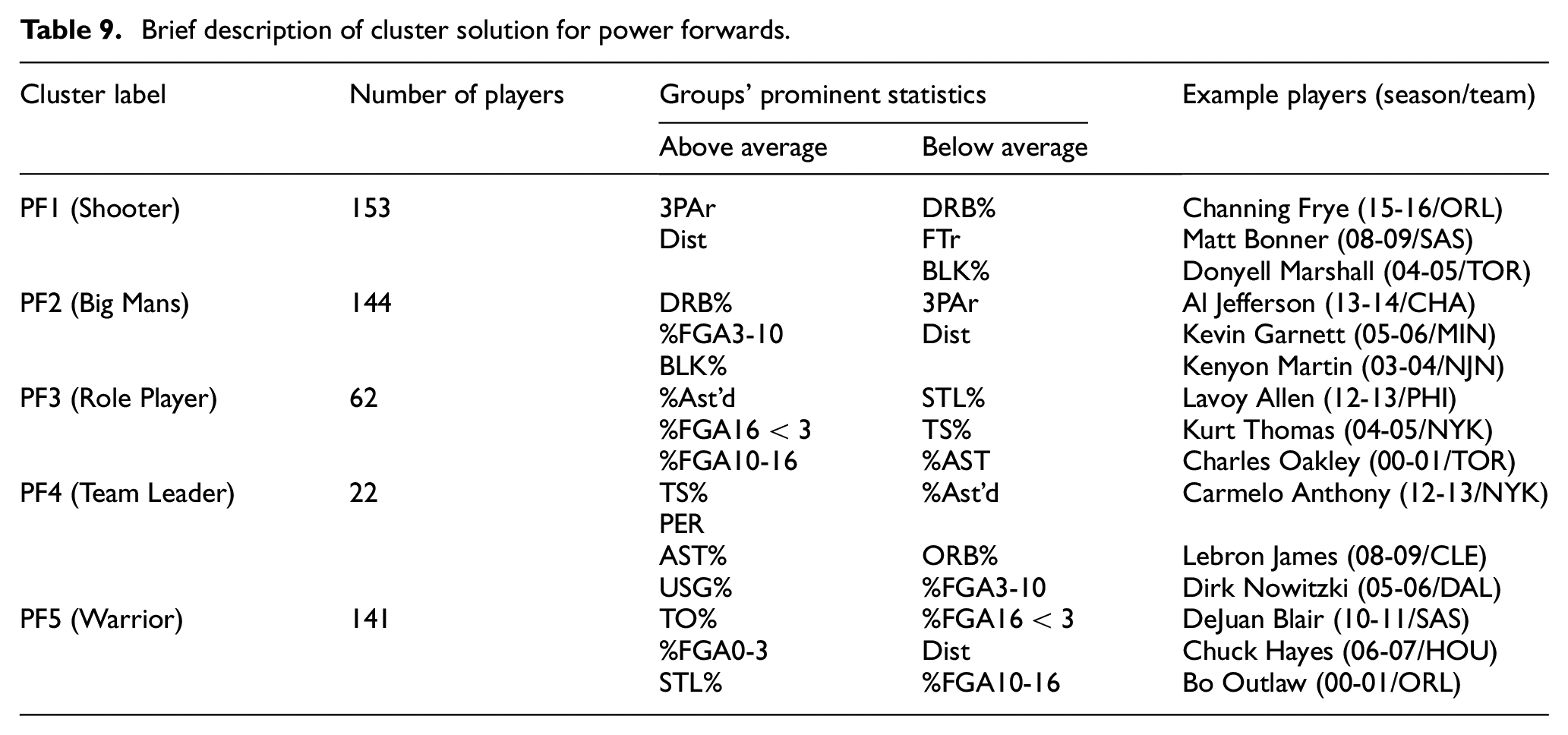
Brief description of cluster solution for power forwards.

Cluster label	Number of players	Groups’ prominent statistics		Example players (season/team)
Cluster label	Number of players	Above average	Below average	Example players (season/team)
PF1 (Shooter)	153	3PAr	DRB%	Channing Frye (15-16/ORL)
		Dist	FTr	Matt Bonner (08-09/SAS)
			BLK%	Donyell Marshall (04-05/TOR)
PF2 (Big Mans)	144	DRB%	3PAr	Al Jefferson (13-14/CHA)
		%FGA3-10	Dist	Kevin Garnett (05-06/MIN)
		BLK%		Kenyon Martin (03-04/NJN)
PF3 (Role Player)	62	%Ast’d	STL%	Lavoy Allen (12-13/PHI)
		%FGA16<3	TS%	Kurt Thomas (04-05/NYK)
		%FGA10-16	%AST	Charles Oakley (00-01/TOR)
PF4 (Team Leader)	22	TS%	%Ast’d	Carmelo Anthony (12-13/NYK)
		PER	%Ast’d	Carmelo Anthony (12-13/NYK)
		AST%	ORB%	Lebron James (08-09/CLE)
		USG%	%FGA3-10	Dirk Nowitzki (05-06/DAL)
PF5 (Warrior)	141	TO%	%FGA16<3	DeJuan Blair (10-11/SAS)
		%FGA0-3	Dist	Chuck Hayes (06-07/HOU)
		STL%	%FGA10-16	Bo Outlaw (00-01/ORL)

Table 10.

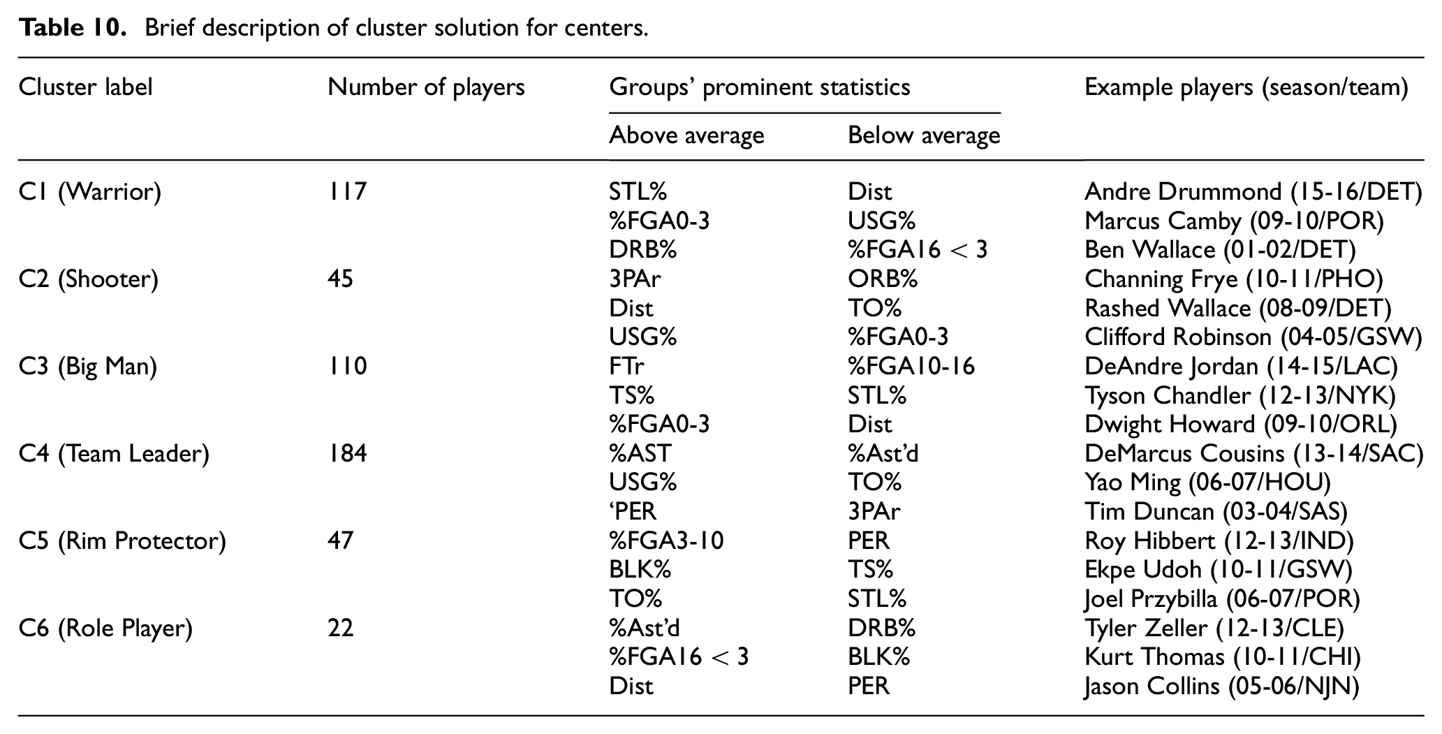
Brief description of cluster solution for centers.

Cluster label	Number of players	Groups’ prominent statistics		Example players (season/team)
Cluster label	Number of players	Above average	Below average	Example players (season/team)
C1 (Warrior)	117	STL%	Dist	Andre Drummond (15-16/DET)
		%FGA0-3	USG%	Marcus Camby (09-10/POR)
		DRB%	%FGA16<3	Ben Wallace (01-02/DET)
C2 (Shooter)	45	3PAr	ORB%	Channing Frye (10-11/PHO)
		Dist	TO%	Rashed Wallace (08-09/DET)
		USG%	%FGA0-3	Clifford Robinson (04-05/GSW)
C3 (Big Man)	110	FTr	%FGA10-16	DeAndre Jordan (14-15/LAC)
		TS%	STL%	Tyson Chandler (12-13/NYK)
		%FGA0-3	Dist	Dwight Howard (09-10/ORL)
C4 (Team Leader)	184	%AST	%Ast’d	DeMarcus Cousins (13-14/SAC)
		USG%	TO%	Yao Ming (06-07/HOU)
		’PER	3PAr	Tim Duncan (03-04/SAS)
C5 (Rim Protector)	47	%FGA3-10	PER	Roy Hibbert (12-13/IND)
		BLK%	TS%	Ekpe Udoh (10-11/GSW)
		TO%	STL%	Joel Przybilla (06-07/POR)
C6 (Role Player)	22	%Ast’d	DRB%	Tyler Zeller (12-13/CLE)
		%FGA16<3	BLK%	Kurt Thomas (10-11/CHI)
		Dist	PER	Jason Collins (05-06/NJN)

Cluster analysis for PG position

In the classic player grouping, the number one position is called the point guard (PG). However, as mentioned previously, the players playing in the same position have different playing styles, so it is not enough to gather them under a single group. In this position, four different styles emerged according to the NbClust analysis.

PG1 “Ball Handler”: This group seems to be the point guard who likes to have the ball in their hand. They find their score by themselves (% Ast’d – 0.241), and their usage rate is high (USG% – 23.22). These are some of the highlights of the group. Jeff Teague from the Atlanta Hawks for the 2015/2016 season is an example of this group.

PG2 “Floor General”: In general, the expectation from the classic point guard is to be the brain of their team. This group includes players who do everything for their team. They are characterized by high assist percentages (AST% – 37.41), efficiency (PER – 19.5), and steals (STL% – 2.836). An example of this group is Chris Paul from the New Orleans Hornets for the 2009/2010 season.

PG3 “Shooter”: The shooting threats have become more critical for modern basketball. Point guards in this group stand out by their shooting ability. The high three-point shooting attempt rates (3PAr – 0.401) and the low free throw attempt rates (FTr – 0.198) are prominent features of this group. Derek Fisher of the Los Angeles Lakers in the 2001/2002 season is an example of this group.

PG4 “Role Player”: The last group of the point guards consists of the members who serve as complementary players of their team. The players in this group do not come to the forefront in specific statistics, but instead take on missionaries’ role in the team’s five. An example of this group is Eric Snow from the Cleveland Cavaliers for the 2005/2006 season.

Cluster analysis for SG position

The second position in basketball is called the shooting guard (SG). Understanding from its name, the expectation from this group is to contribute points to the team. However, this is a statement too general for all players who play in this position. So, this study suggests four different groups.

SG1 “Shooter”: The players in this group stand out as the sharpshooter of their teams. They have high three-point shooting attempt rates (3PAr – 0.438), and their true shooting percentage is high (TS% – 0.552). The low rate of going to the foul line (FTr – 0.222) due to their playing style is another feature of this group. Kyle Korver from the Atlanta Hawks for the 2014/2015 season is an example of this group.

SG2 “Warrior”: Some players play more physical games and contribute to their teams with hustle plays. This type of player forms this group. The high offensive rebound percentage (ORB% – 5.950) and the high block percentage (BLK% – 1.143) highlight this group. An example of this group is Bonzi Wells from the Sacramento Kings for the 2005/2006 season.

SG3 “Role Player”: The players in this group act as complementary players of the team, which do not stand out with their specific features. Jeff McInnis of the Charlotte Bobcats in the 2007/2008 season is an example of this group.

SG4 “Team Leader”: The last group of the shooting guards consists of players who are candidates for being a team star. The players in this group like using the ball (USG% – 25.977) and play with high efficiency (PER – 18.822). An example of this group is Kobe Bryant from the Los Angeles Lakers for the 2004/2005 season.

Cluster analysis for SF position

The third position in basketball is called the small forward (SF). One of the two forward positions is usually called by this name because it is played by shorter players. Of course, this naming has no relation to the style of play. This study, based on playing styles, suggests four different groups.

SF1 “Team Leader”: The team’s star candidates are included in this group for this position. As in the SG position, this group stands out with its high efficiency (PER – 18.531) and high usage rate (USG% – 25.302) values. Lebron James from the Cleveland Cavaliers for the 2008/2009 season is an example of this group.

SF2 “Shooter”: With high three-point shooting attempt rates (3PAr – 0.445), high true shooting percentage (TS% – 0.545), and low free throw rate (FTr – 0.209), these features are characteristics of the group called the shooter. An example of this group is DeShawn Stevenson from the Atlanta Hawks for the 2012/2013 season.

SF3 “Warrior”: The players with more physical strength-based play styles compose this group. They get most of the points by driving into the paint (Dist – 9.745), and they also contribute to their team with a high offensive rebound percentage (ORB% – 6.416) and block percentage (BLK% – 1.897). Andrei Kirilenko of the Utah Jazz in the 2001/2002 season is an example of this group.

SF4 “Role Player”: As in other positions, there are no prominent statistics in this group, which are categorized as role players. An example of this group is Alvin Williams from the Toronto Raptors for the 2003/2004 season.

Cluster analysis for PF position

The second forward position in basketball is called the power forward (PF). The traditional expectation for this position is to play close to the rim. However, this expectation changed with the evolution of the game. This study proposed to divide the power forwards into five different groups.

PF1 “Shooter”: Big men with shooting ability can give their teams a great advantage. The players in this group also deserve to take the name shooter with high three-point shooting attempt rates (3PAr – 0.310), average shooting rage distance (Dist – 13.816), and low free throw rate (FTr – 0.247). Donyell Marshall from the Toronto Raptors for the 2004/2005 season is an example of this group.

PF2 “Big Man”: It seems that the players in this group play closer to the rim (Dist – 9.108). They play both the offensive (PER – 20.547) and defensive part (DRB% – 22.015) of the game. An example of this group is Kevin Garnett from the Minnesota Timberwolves for the 2005/2006 season.

PF3 “Role Player”: In this group called the role player, players act as the complementary element of the teams. Lavoy Allen of the Philadelphia Sixers in the 2012/2013 season is an example of this group.

PF4 “Team Leader”: Star players of some teams can be their big men. This group has some prominent features (PER – 25.3, TS% – 0.592). An example of this group is Dirk Nowitzki from the Dallas Mavericks for the 2005/2006 season.

PF5 “Warrior”: The players who make up the last forward group consist of players who try to contribute to their teams with other features (STL% – 1.601), rather than using balls (USG% – 16.604). An example of this group is DeJuan Blair from the San Antonio Spurs for the 2010/2011 season.

Cluster analysis for C position

The last position in basketball is called the center (C). In the traditional positions, big and tall players are gathered under this group. However, this grouping is made only according to their size. In this study, six different styles emerged according to the NbClust analysis.

C1 “Warrior”: The players in this group, created for the center position as in power forward, contribute to their teams in other areas (STL% – 1.452, DRB% – 22.332), instead of using the ball much (USG% – 15.311). Ben Wallace from the Detroit Pistons for the 2001/2002 season is an example of this group.

C2 “Shooter”: Shooting for big men is often difficult, but players in this group can achieve it. The players in this group prefer to play behind the three-point line (3PAr – 0.322, Dist – 14.891). An example of this group is Channing Frye from the Phoenix Suns for the 2010/2011 season.

C3 “Big Man”: This group consists of players who are centers in the classical sense, that is, they use the painted area well (TS% – 0.590) and play close to the rim (Dist – 3.484, %FGA0-3 – 0.623). Dwight Howard of the Orlando Magic in the 2009/2010 season is an example of this group.

C4 “Team Leader”: Despite being at the center position, the players who take the game’s lead are included in this group. Besides their high efficiency (PER – 19.628), they deserve the leader name with a high assist percentage (AST% – 12.062). An example of this group is Tim Duncan from the San Antonio Spurs for the 2003/2004 season.

C5 “Rim Protector”: The main job of players in this group is to keep opponents away from the rim (BLK% – 4.664). It can also be said that their interaction with the ball is not very good (TO% – 16.983). An example of this group is Roy Hibbert from the Indiana Pacers for the 2012/2013 season.

C6 “Role Player”: The players in the last group for the center position are role players. It mainly consists of players who work for the team and find their points through assists. An example of this group is Jason Collins from the New Jersey Nets for the 2005/2006 season.

Discussion

It is undeniable that players must perform well in order to win. However, as stated by Pérez-Toledano et al.,⁹⁰ in team sports such as basketball, the team’s overall value cannot be obtained by simply evaluating and summing the player’s performances. Also, Sampaio et al.⁹¹ stated that it is essential for team performance to evaluate player performances according to their positions and reveal the players’ characteristics that complement each other. In this study, rather than evaluating players’ efficiency, player styles according to their positions, which is thought to be helpful when examining the team’s harmony, were clarified.

In previous studies, five positions were considered insufficient for today’s basketball, and new positions were offered through clustering studies.^44–47 However, basketball is played with five people on the court, and the performance of these five players determines the victory. In other words, team chemistry is fundamental in evaluating the success of the team.⁹² Therefore, calculating the harmony of these five is also vital to determine team success. Nevertheless, it is complicated to analyze this situation, as there are too many possible five-player lineup combinations.⁹³ In this study, instead of suggesting new positions, the players were clustered in their positions, which would provide a manageable number of lineup combinations when examining team harmony. As a result of the analysis, four clusters for PG, SG, and SF positions, five clusters for PF position, and six clusters for C position were assigned. Since there was not enough data to analyze the compatibility of a full lineup, the individual and dual achievements of the groups were evaluated.

The effect of clusters

The team success criteria had to be assigned to examine the effects of the clusters on winning and losing. Point differential was mentioned as one of the most used metrics for game performance indicators in the study by Huyghe et al.⁹⁴ For examining the clusters’ effects, a net point differential per 48 min was used, and the results of the 565 lineups included in the data set were checked. Adjusted plus-minus (APM), average points differential, and the percentage of clusters on winning teams were analyzed while determining the prominent clusters. These three results were expected to support each other, and they were checked to reach a more precise result. Plus-minus (+/−) is a rating that presents the net changes in the score when a given player is on the court, and the APM is a regression-based version of the PM rating.⁹⁵ In this study, clusters were considered as a member of the same team, and APM values were calculated. The second metric is the average points differential, which is an arithmetic mean of a cluster’s net point differential results. Finally, while calculating the winning percentage, negative points differences were taken as losses, positive point differences as winning. The winning percentage of the whole dataset was calculated as 70.1%.

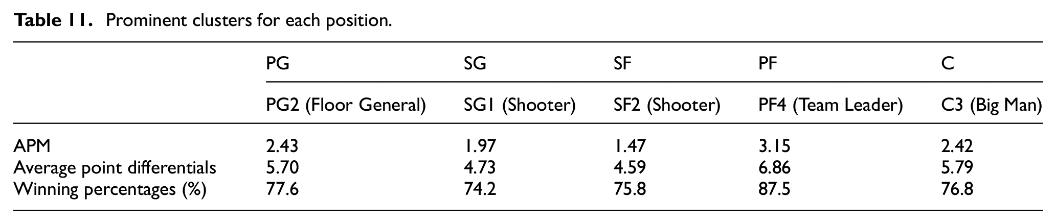
Table 11 shows the prominent clusters for each position. It was observed that these clusters received the highest score in all three metrics used in the evaluation. The PG2 group showed up in 76 rotations, 59 of which were the winning teams. This group played with a 2.43 APM and a 5.70 average point differential. The players of this cluster, which stood out with its high assist percentages (AST%) and steal percentages (STL%), were more involved in winning teams than other PG clusters. In SG and SF positions, SG1 and SF2 clusters had very close values. Respectively, they appeared in the winning teams 161 and 141 times and reached a 1.97 and 1.47 average point differential with a 4.73 and 4.59 APM. For both of these positions, it was seen that the groups of players called shooter, who used more three-point shots and had a high true shooting percentage (TS%), were more often on the winning teams. The PF4 group was the cluster that stood out the most in its position. Except for a high winning percentage, they got 3.15 APM and a 6.86 average point differential. It is noteworthy that these cluster players, who were more on the winning teams, used the ball more (USG%) and played with high efficiency (PER). For the last position, the C3 cluster stood out with 2.42 APM and a 5.79 average point differential. This group appeared in 138 games, including 106 for winning teams.

Table 11.

Prominent clusters for each position.

	PG	SG	SF	PF	C
	PG2 (Floor General)	SG1 (Shooter)	SF2 (Shooter)	PF4 (Team Leader)	C3 (Big Man)
APM	2.43	1.97	1.47	3.15	2.42
Average point differentials	5.70	4.73	4.59	6.86	5.79
Winning percentages (%)	77.6	74.2	75.8	87.5	76.8

The effect of pairs

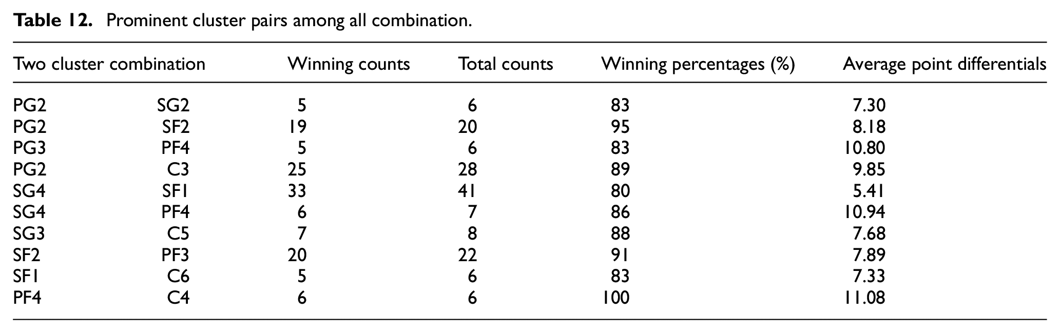
As previously mentioned, how players play with each other in basketball is a crucial factor for success. Even if the players’ efficiency was analyzed with APM, another aim of this study was to establish the basis for examining the compatibility of five players. Since the five-player combinations were not seen in sufficient numbers in the data collected, the effects of the two-player combination were examined. Among the pairs created for all positions, the ones with the highest average points differential are given in Table 12, with counts and the percentage of pairs on winning teams. It seems that the PG2 cluster stood out among the duos with the point guards. With all other positions, except for the power forward position, the PG2 cluster was the best fit. This result was not surprising as the PG2 cluster was also prominent in the individual cluster analysis. Best combination with point guard position, PG2 and SF2 duo stood out with a 95% winning percentage. For the pairs with the scoring guards, the result was surprising. The SG1 cluster, which came to the forefront in the individual analysis, lagged behind in terms of compatibility in dual examinations. While all other clusters appeared in successful pairs, cluster SG1 was not seen. In pairs with small forwards, it was observed that the SF1 group had good compatibility in pairs with the SF2 group, which also stood out in the individual analysis. The 91% winning percentage achieved by the SF2 cluster and the PF3 cluster was remarkable. The PF4 cluster, which also stood out in the individual analysis, came to the forefront in pairs with power forwards. The PF4 and C4 duo, both called the team leader, drew attention by only taking part in the winning teams. Finally, all other clusters were included in successful duos in pairs with center position, except for C1 and C2 groups.

Table 12.

Prominent cluster pairs among all combination.

Two cluster combination		Winning counts	Total counts	Winning percentages (%)	Average point differentials
PG2	SG2	5	6	83	7.30
PG2	SF2	19	20	95	8.18
PG3	PF4	5	6	83	10.80
PG2	C3	25	28	89	9.85
SG4	SF1	33	41	80	5.41
SG4	PF4	6	7	86	10.94
SG3	C5	7	8	88	7.68
SF2	PF3	20	22	91	7.89
SF1	C6	5	6	83	7.33
PF4	C4	6	6	100	11.08

Conclusion

If teams want to succeed, they must bring together players that are compatible with each other. For this, it is essential to define the players’ game types correctly. In this study, players were grouped according to their playing styles. While doing this, the reality that basketball is played with five people on the court was not ignored. Players were grouped in each of the five traditional positions, taking into account the 15 NBA seasons. A data set was created for this grouping with 17 game-related statistics, which reflect the player’s game style. The hierarchical clustering method was used as the clustering method, and internal validity indexes were compared to determine the optimum number of groups. As a result, four different clusters were formed for the point guards, shooting guards, and small forwards, five different clusters for the power forwards, and six different clusters for the center position. These clusters created for each position were defined according to their prominent statistics and labeled for general information purposes (Shooter, Role Player, Team Leader, etc.).

The individual achievements of the formed clusters were also examined in the study. Based on three performance indicators (adjusted plus-minus (APM), average points differential, and the percentage of clusters on winning teams), PG2 (Floor General), SG1 (Shooter), SF2 (Shooter), PF4 (Team Leader), and C3 (Big Man) were found as clusters that stood out in their positions. Since it is evident that individuality will not be enough in team sports such as basketball, the achievements of pairs were also examined. Some clusters that were successful in the individual cluster analysis were also successful in the pairwise analysis (such as PG1 and PF4 clusters). However, although some clusters did not come to the forefront in the individual analysis, they seemed to distinguish themselves when they played together with the right group of players. For example, SG4 and SF1 clusters, which were not included as the best in the individual analysis mentioned in Section 4.1, stood out with an 80% winning percentage and a 5.41 average points differential when played together.

The main focus of this research was to cluster the players according to their playing style for each position. In this way, coaches would be able to analyze the player styles in their teams more easily. While the player’s pairs analysis would provide the coaches with an idea about the harmony between their players, the team compatibility analysis that is planned in future work will also support the team formation. NBA front offices can benefit from this work when renewing player contracts and determining free agency strategies.

There were some limitations of this study. Firstly, only the NBA data was used in the analysis. Therefore, only players who played in the NBA were included in the study. By adding the statistics from The National Collegiate Athletic Association (NCAA) and international leagues to this study, the analysis of the NBA draft can be accomplished. Also, in this way, international league teams can benefit from this work. Secondly, only statistical data was used when clustering players. The mental data, known to affect the game, could not be obtained, and there was no possibility of obtaining these data by testing the players. More successful groups could be created if the mental characteristics of the players are added to the analysis.

The individual and pairs achievements of the formed groups were also included in this study. Future studies are planned to analyze the harmony of created clusters and determine the results of these clusters when they play with each other. These efforts will establish a decision support system that will suggest which type of player should be replaced when a player leaves the team and/or indicate which position has the most impact on disrupting team compatibility, thus requiring changes to achieve better results. In addition, it is planned to include the team budgets, which is an essential constraint in team building, into the decision support system. Hence, it is guaranteed that recommended players would meet the team budget constraint. As another future study, based on team statistics, the game styles of the coaches can be determined by clustering and can be included in the system while examining team harmony. While in this study, the playing styles of the players were examined separately for each season, a system that examines players’ game developments and predicts their playing styles for the next season can be integrated with future research.

Footnotes

Appendix

Table A6.

The means and standard deviation of C clusters.

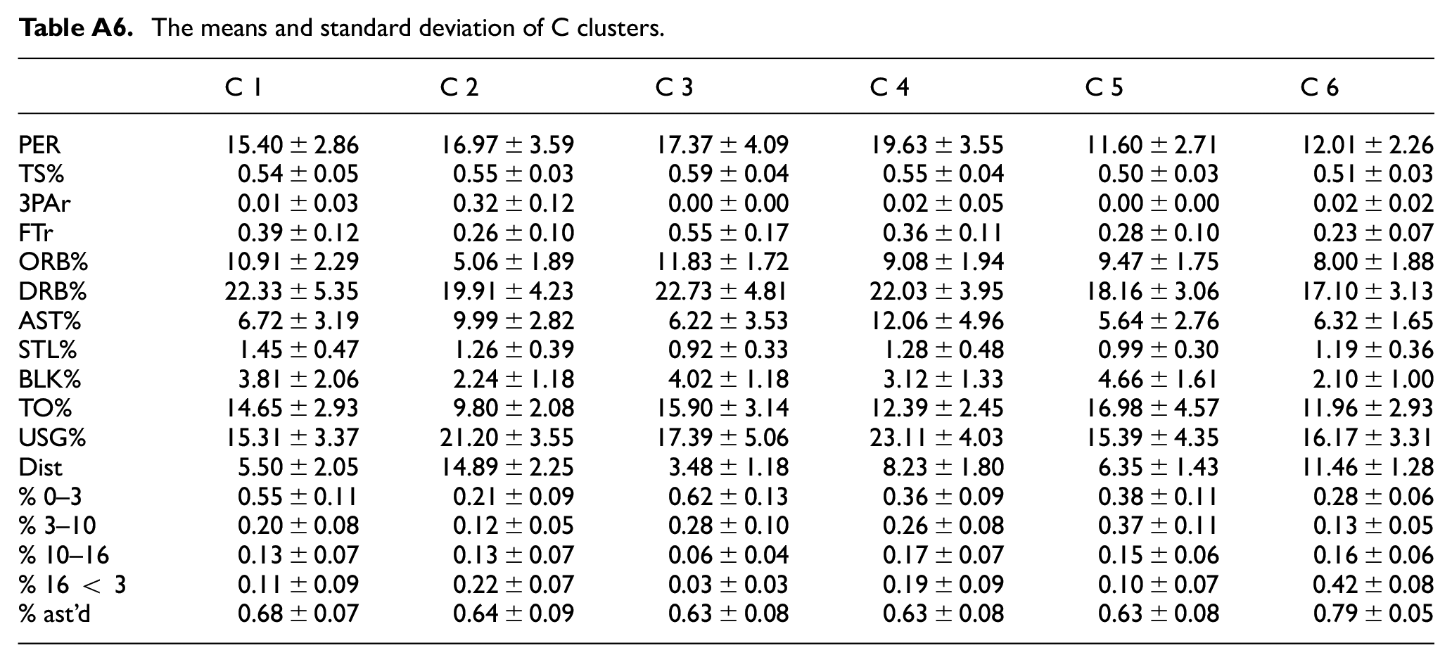
	C 1	C 2	C 3	C 4	C 5	C 6
PER	15.40 ± 2.86	16.97 ± 3.59	17.37 ± 4.09	19.63 ± 3.55	11.60 ± 2.71	12.01 ± 2.26
TS%	0.54 ± 0.05	0.55 ± 0.03	0.59 ± 0.04	0.55 ± 0.04	0.50 ± 0.03	0.51 ± 0.03
3PAr	0.01 ± 0.03	0.32 ± 0.12	0.00 ± 0.00	0.02 ± 0.05	0.00 ± 0.00	0.02 ± 0.02
FTr	0.39 ± 0.12	0.26 ± 0.10	0.55 ± 0.17	0.36 ± 0.11	0.28 ± 0.10	0.23 ± 0.07
ORB%	10.91 ± 2.29	5.06 ± 1.89	11.83 ± 1.72	9.08 ± 1.94	9.47 ± 1.75	8.00 ± 1.88
DRB%	22.33 ± 5.35	19.91 ± 4.23	22.73 ± 4.81	22.03 ± 3.95	18.16 ± 3.06	17.10 ± 3.13
AST%	6.72 ± 3.19	9.99 ± 2.82	6.22 ± 3.53	12.06 ± 4.96	5.64 ± 2.76	6.32 ± 1.65
STL%	1.45 ± 0.47	1.26 ± 0.39	0.92 ± 0.33	1.28 ± 0.48	0.99 ± 0.30	1.19 ± 0.36
BLK%	3.81 ± 2.06	2.24 ± 1.18	4.02 ± 1.18	3.12 ± 1.33	4.66 ± 1.61	2.10 ± 1.00
TO%	14.65 ± 2.93	9.80 ± 2.08	15.90 ± 3.14	12.39 ± 2.45	16.98 ± 4.57	11.96 ± 2.93
USG%	15.31 ± 3.37	21.20 ± 3.55	17.39 ± 5.06	23.11 ± 4.03	15.39 ± 4.35	16.17 ± 3.31
Dist	5.50 ± 2.05	14.89 ± 2.25	3.48 ± 1.18	8.23 ± 1.80	6.35 ± 1.43	11.46 ± 1.28
% 0–3	0.55 ± 0.11	0.21 ± 0.09	0.62 ± 0.13	0.36 ± 0.09	0.38 ± 0.11	0.28 ± 0.06
% 3–10	0.20 ± 0.08	0.12 ± 0.05	0.28 ± 0.10	0.26 ± 0.08	0.37 ± 0.11	0.13 ± 0.05
% 10–16	0.13 ± 0.07	0.13 ± 0.07	0.06 ± 0.04	0.17 ± 0.07	0.15 ± 0.06	0.16 ± 0.06
% 16 < 3	0.11 ± 0.09	0.22 ± 0.07	0.03 ± 0.03	0.19 ± 0.09	0.10 ± 0.07	0.42 ± 0.08
% ast’d	0.68 ± 0.07	0.64 ± 0.09	0.63 ± 0.08	0.63 ± 0.08	0.63 ± 0.08	0.79 ± 0.05

Declaration of conflicting interests

The author(s) declared no potential conflicts of interest with respect to the research, authorship, and/or publication of this article.

Funding

The author(s) disclosed receipt of the following financial support for the research, authorship, and/or publication of this article: This study was funded by Marmara University Scientific Research Project Coordination Unit under project number FEN-C-DRP-120417-0181.

ORCID iD

Eyüp Anıl Duman

References

Chen

Liao

. Identifying standards for postseason advancement: a case of the National Basketball Association. Int Trans Oper Res 2021; 28: 2359–2376.

Kekez

Ćukušić

Jadrić

. Data mining approach for business value analysis in basketball. Zb Veleuč Rij 2021; 9: 227–248.

Ibanez

Sampaio

Saenz-Lopez

, et al. Game statistics discriminating the final outcome of Junior World Basketball Championship matches (Portugal 1999). J Hum Mov Stud 2003; 45: 1–19.

Ibáñez

Sampaio

Feu

, et al. Basketball game-related statistics that discriminate between teams’ season-long success. Eur J Sport Sci 2008; 8: 369–372.

Angel Gómez

Lorenzo

Sampaio

, et al. Game-related statistics that discriminated winning and losing teams from the Spanish men’s professional basketball teams. Coll Antropol 2008; 32: 451–456.

Csataljay

O’Donoghue

Hughes

, et al. Performance indicators that distinguish winning and losing teams in basketball. Int J Perform Anal Sport 2009; 9: 60–66.

Lorenzo

Gómez

MÁ

Ortega

, et al. Game related statistics which discriminate between winning and losing under-16 male basketball games. J Sci Med Sport 2010; 9: 664–668.

Puente

Coso

Salinero

, et al. Basketball performance indicators during the ACB regular season from 2003 to 2013. Int J Perform Anal Sport 2015; 15: 935–948.

Çene

. What is the difference between a winning and a losing team: insights from Euroleague basketball. Int J Perform Anal Sport 2018; 18: 55–68.

10.

Mikołajec

Banyś

Żurowska-Cegielska

, et al. How to win the basketball Euroleague? Game performance determining sports results during 2003-2016 matches. J Hum Kinet 2021; 77: 287–296.

11.

Raval

KMR

Pagaduan

. Factors that differentiate winning and losing in men’s university basketball. Montenegrin J Sports Sci Med 2021; 10: 13–17.

12.

Junior

DDR

. Statistical analysis of basketball performance indicators according to home/away games and winning and losing teams. J Hum Mov Stud 2004; 47: 327–336.

13.

García

Ibáñez

Gómez

, et al. Basketball game-related statistics discriminating ACB league teams according to game location, game outcome and final score differences. Int J Perform Anal Sport 2014; 14: 443–452.

14.

Gòmez

MÁ

Lorenzo

Ortega

, et al. Game related statistics discriminating between starters and nonstarters players in women’s National Basketball Association League (WNBA). J Sci Med Sport 2009; 8: 278–283.

15.

Moreno

Gómez

Lago

, et al. Effects of starting quarter score, game location, and quality of opposition in quarter score in elite women’s basketball. Kinesiology 2013; 45: 48–54.

16.

Gómez

MÁ

Silva

Lorenzo

, et al. Exploring the effects of substituting basketball players in high-level teams. J Sports Sci 2017; 35: 247–254.

17.

Zhang

Lorenzo

Zhou

, et al. Performance profiles and opposition interaction during game-play in elite basketball: evidences from National Basketball Association. Int J Perform Anal Sport 2019; 19: 28–48.

18.

Dong

Lian

Zhang

, et al. Addressing opposition quality in basketball performance evaluation. Int J Perform Anal Sport 2021; 21: 263–276.

19.

Teramoto

Cross

. Relative importance of performance factors in winning NBA games in regular season versus playoffs. J Quant Anal Sports 2010; 6: 1–19.

20.

Dogan

Ersoz

. The important game-related statistics for qualifying next rounds in Euroleague. Montenegrin J Sports Sci Med 2019; 8: 43–50.

21.

Stavropoulos

Kolias

Papadopoulou

, et al. Game related predictors discriminating between winning and losing teams in preliminary, second and final round of basketball world cup 2019. Int J Perform Anal Sport 2021; 21: 383–395.

22.

Giovanini

Conte

Ferreira-Junior

, et al. Assessing the key game-related statistics in Brazilian professional basketball according to season phase and final score difference. Int J Perform Anal Sport 2021; 21: 295–305.

23.

Kubatko

Oliver

Pelton

, et al. A starting point for analyzing basketball statistics. J Quant Anal Sports 2007; 3: 1–22.

24.

Sarlis

Tjortjis

. Sports analytics — evaluation of basketball players and team performance. Inf Syst 2020; 93: 101562.

25.

Wright

. 50 years of OR in sport. J Oper Res Soc 2009; 60: S161–S168.

26.

K-t

Z-x

Zhuang

R-C

. An exploratory study of long-term performance evaluation for elite basketball players. Int J Space Sci Eng 2008; 2: 195–203.

27.

Dadelo

Turskis

Zavadskas

, et al. Multi-criteria assessment and ranking system of sport team formation based on objective-measured values of criteria set. Expert Syst Appl 2014; 41: 6106–6113.

28.

Ballı

Korukoğlu

. Development of a fuzzy decision support framework for complex multi-attribute decision problems: a case study for the selection of skilful basketball players. Expert Syst 2014; 31: 56–69.

29.

Pradhan

Chachad

. Re-ranking regular seasons in the National Basketball Association’s modern era: a replication and extension of Pradhan (2018). J Stat Manag Syst 2021; 2021: 1–20.

30.

Cooper

Ruiz

Sirvent

. Selecting non-zero weights to evaluate effectiveness of basketball players with DEA. Eur J Oper Res 2009; 195: 563–574.

31.

Lee

Worthington

. A note on the ‘Linsanity’ of measuring the relative efficiency of National Basketball Association guards. Appl Econ 2013; 45: 4193–4202.

32.

Radovanovic

Radojicic

Savic

. Two-phased DEA-MLA approach for predicting efficiency of NBA players. Yugoslav J Operations Res 2014; 24: 347–358.

33.

Assani

Mansoor

Asghar

, et al. Efficiency, RTS, and marginal returns from salary on the performance of the NBA players: a parallel DEA network with shared inputs. J Ind Manag Optim 2021; 0: 0.

34.

Trninić

Dizdar

. System of the performance evaluation criteria weighted per positions in the basketball game. Coll Antropol 2000; 24: 217–234.

35.

Dezman

Trninić

Dizdar

. Expert model of decision-making system for efficient orientation of basketball players to positions and roles in the game – empirical verification. Coll Antropol 2001; 25: 141–152.

36.

Page

Fellingham

Reese

. Using box-scores to determine a position’s contribution to winning basketball games. J Quant Anal Sports 2007; 3: 1.

37.

Mateus

Gonçalves

Abade

, et al. Game-to-game variability of technical and physical performance in NBA players. Int J Perform Anal Sport 2015; 15: 764–776.

38.

Rangel

Ugrinowitsch

Lamas

. Basketball players’ versatility: assessing the diversity of tactical roles. Int J Sports Sci Coach 2019; 14: 552–561.

39.

Zhang

Lorenzo

Gómez

, et al. Clustering performances in the NBA according to players’ anthropometric attributes and playing experience. J Sports Sci 2018; 36: 2511–2520.

40.

Mateus

Esteves

Gonçalves

, et al. Clustering performance in the European basketball according to players’ characteristics and contextual variables. Int J Sports Sci Coach 2020; 15: 405–411.

41.

Zhang

Liu

, et al. Application of K-means clustering algorithm for classification of NBA guards. Int J Sci Eng Appl 2016; 5(1): 1–6.

42.

Bianchi

Facchinetti

Zuccolotto

. Role revolution: towards a new meaning of positions in basketball. Electron J Appl Stat Anal 2017; 10: 712–734.

43.

Patel

. Clustering professional basketball players by performance. Los Angeles, CA: UCLA, 2017.

44.

Diambra

. Using topological clustering to identify emerging positions and strategies in NCAA men’s basketball. Knoxville, TN: University of Tennessee, 2018.

45.

Lutz

. A cluster analysis of NBA players. In: MIT Sloan sports analytics conference, Boston, MA, 2–3 March 2012.

46.

Alagappan

. From 5 to 13: Redefining the positions in basketball. In: MIT Sloan sports analytics conference, Boston, MA, 2–3 March 2012.

47.

Kalman

Bosch

. NBA lineup analysis on clustered player tendencies: A new approach to the positions of basketball & modeling lineup efficiency of soft lineup aggregates. In: MIT Sloan Sports Analytics Conference, Boston, MA, 6–7 March 2020.

48.

Basketball-Reference. Basketball statistics and history, http://basketball-reference.com (accessed 1 September 2016).

49.

R Core Team. R: a language and environment for statistical computing. Vienna, Austria: R Foundation for Statistical Computing, 2021.

50.

NBA. The official site of the National Basketball Association, www.nba.com/stats (accessed 15 September 2016).

51.

Oliver

. Basketball on paper: rules and tools for performance analysis. Dulles, VA: Potomac Books, Inc, 2004.

52.

Ferreira

Hitchcock

. A comparison of hierarchical methods for clustering functional data. Commun Stat Simul Comput 2009; 38: 1925–1949.

53.

Hands

Everitt

. A Monte Carlo study of the recovery of cluster structure in binary data by hierarchical clustering techniques. Multivariate Behav Res 1987; 22: 235–243.

54.

Blashfield

. Mixture model tests of cluster analysis: accuracy of four agglomerative hierarchical methods. Psychol Bull 1976; 83: 377–388.

55.

Charrad

Ghazzali

Boiteau

, et al. NbClust: AnRPackage for determining the relevant number of clusters in a data set. J Stat Softw 2014; 61: 1–36.

56.

Murtagh

Legendre

. Ward’s hierarchical agglomerative clustering method: which algorithms implement Ward’s criterion? J Classif 2014; 31: 274–295.

57.

Tan

P-N

. Introduction to data mining. New Delhi: Pearson Education India, 2006.

58.

Arbelaitz

Gurrutxaga

Muguerza

, et al. An extensive comparative study of cluster validity indices. Pattern Recognit 2013; 46: 243–256.

59.

Calinski

Harabasz

. A dendrite method for cluster analysis. Commun Stat Theory Methods 1974; 3: 1–27.

60.

Duda

Hart

. Pattern classification and scene analysis. New York, NY: John Wiley & Sons, 1973.

61.

Hubert

Levin

. A general statistical framework for assessing categorical clustering in free recall. Psychol Bull 1976; 83: 1072–1080.

62.

Baker

Hubert

. Measuring the power of hierarchical cluster analysis. J Am Stat Assoc 1975; 70: 31–38.

63.

Beale

EML

. Euclidean cluster analysis. London: Scientific Control Systems Limited, 1969.

64.

Sarle

. Cubic clustering criterion. Technical report A-108, 1983. Cary, NC: SAS Institute Inc.

65.

Kraemer

. Biserial correlation. In: Kotz

Johnson

Read

(eds) Encyclopedia of statistical sciences. New York, NY: Wiley, 1982, pp.276–279, Vol. 1.

66.

Rohlf

. Methods of comparing classifications. Annu Rev Ecol Syst 1974; 5(1): 101–113.

67.

Davies

Bouldin

. A cluster separation measure. IEEE Trans Pattern Anal Mach Intell 1979; 1: 224–227.

68.

Frey

van Groenewoud

. A cluster analysis of the D 2 matrix of white spruce stands in Saskatchewan based on the maximum-minimum principle. J Ecol 1972; 60: 873–886.

69.

Hartigan

. Clustering algorithms. New York, NY: Wiley, 1975.

70.

Ratkowsky

Lance

. Criterion for determining the number of groups in a classification. Aust Comput J 1978; 10: 115–117.

71.

Scott

Symons

. Clustering methods based on likelihood ratio criteria. Biometrics 1971; 27: 387–397.

72.

Marriott

FHC

. Practical problems in a method of cluster analysis. Biometrics 1971; 27: 501–514.

73.

Ball

Hall

. ISODATA, a novel method of data analysis and pattern classification. Menlo Park, CA: Stanford Research Institute, 1965.

74.

Milligan

Cooper

. An examination of procedures for determining the number of clusters in a data set. Psychometrika 1985; 50: 159–179.

75.

Edwards

Cavalli-Sforza

. A method for cluster analysis. Biometrics 1965; 21: 362–375.

76.

Friedman

Rubin

. On some invariant criteria for grouping data. J Am Stat Assoc 1967; 62: 1159–1178.

77.

McClain

Rao

. Clustisz: a program to test for the quality of clustering of a set of objects. J Mark Res 1975; 12: 456–460.

78.

Krzanowski

Lai

. A criterion for determining the number of groups in a data set using sum-of-squares clustering. Biometrics 1988; 44: 23–34.

79.

Rousseeuw

. Silhouettes: a graphical aid to the interpretation and validation of cluster analysis. J Comput Appl Math 1987; 20: 53–65.

80.

Tibshirani

Walther

Hastie

. Estimating the number of clusters in a data set via the gap statistic. J R Stat Soc Ser B 2001; 63: 411–423.

81.

Lebart

Morineau

Piron

. Statistique exploratoire multidimensionnelle. Paris: Dunod, 1995.

82.

Dunn

. Well-separated clusters and optimal fuzzy partitions. J Cybern 1974; 4: 95–104.

83.

Hubert

Arabie

. Comparing partitions. J Classif 1985; 2: 193–218.

84.

Halkidi

Vazirgiannis

Batistakis

. Quality scheme assessment in the clustering process. In: European conference on principles of data mining and knowledge discovery, PKDD 2000, Lyon, France, 13–6 September 2000.

85.

Halkidi

Vazirgiannis

. Clustering validity assessment: Finding the optimal partitioning of a data set. In: IEEE international conference on data mining, San Jose, CA, 29 November–2 December 2001.

86.

Guerra

Robles

Bielza

, et al. A comparison of clustering quality indices using outliers and noise. Intell Data Anal 2012; 16: 703–715.

87.

Mufti

Bertrand

El Moubarki

. Decomposition of the Rand index in order to assess both the stability and the number of clusters of a partition. Pattern Recognit Lett 2012.

88.

Chan

. Prediction of hourly solar radiation with multi-model framework. Energy Convers Manag 2013; 76: 347–355.

89.

Chouikhi

Charrad

Ghazzali

. A comparison study of clustering validity indices. In: 2015 Global summit on computer & information technology (GSCIT), Sousse, Tunisia, 11–13 June 2015. New York, NY: IEEE.

90.

Pérez-Toledano

MÁ

Rodriguez

García-Rubio

, et al. Players’ selection for basketball teams, through performance index rating, using multiobjective evolutionary algorithms. PLoS One 2019; 14: e0221258.

91.

Sampaio

Janeira

Ibáñez

, et al. Discriminant analysis of game-related statistics between basketball guards, forwards and centres in three professional leagues. Eur J Sport Sci 2006; 6: 173–178.

92.

Berri

Jewell

. Wage inequality and firm performance: professional basketball’s natural experiment. Atl Econ J 2004; 32: 130–139.

93.

Maymin

Shen

. NBA chemistry: positive and negative synergies in basketball. Int J Comput Sci Sport 2013; 12: 4–23.

94.

Huyghe

Alcaraz

Calleja-González

, et al. The underpinning factors of NBA game-play performance: a systematic review (2001-2020). Phys Sportsmed. Epub ahead of print 15 April 2021. DOI: 10.1080/00913847.2021.1896957

95.

Grassetti

Bellio

Di Gaspero

, et al. An extended regularized adjusted plus-minus analysis for lineup management in basketball using play-by-play data. IMA J Manag Math 2021; 32: 385–409.

A cluster analysis of basketball players for each of the five traditionally defined positions

Abstract

Keywords

Introduction

Methods

Sample

Variables

Procedure and data analysis

Results

Cluster analysis for PG position

Cluster analysis for SG position

Cluster analysis for SF position

Cluster analysis for PF position

Cluster analysis for C position

Discussion

The effect of clusters

The effect of pairs

Conclusion

Footnotes

Appendix

Declaration of conflicting interests

Funding

ORCID iD

References