Sage Journals: Discover world-class research

Abstract

The development hardware and software aspects of a novel system for monitoring performance in the strength and conditioning domain are summarized in this paper. A development framework is presented to enable the capture of development processes and support detailed comparison of performance monitoring systems. The framework couples the established Computer Integrated Manufacture Open Systems Architecture (CIMOSA) with Unified Modelling Language (UML) to document both the software development and implementation. Corrective algorithms are proposed that have increased the accuracy of the IMU outputs in monitoring the performance of a countermovement jump. Lastly, a wireless Inertial Measurement Unit (IMU) has been validated for use within the strength and conditioning domain by comparison with an optical motion capture reference measure.

Keywords

Countermovement CIMOSA IMU performance monitoring framework architecture

Introduction

Strength and conditioning (S&C) feedback systems are important tools used by coaches and athletes participating in a broad range of sports.^1–5 These systems capture data related to performance monitoring techniques, such as vertical jumps (e.g. countermovement jumps (CMJ) and squat jumps (SJ)) to identify changes in technique, fatigue and differences between athletic populations.⁶ Typically, maximum CMJ height (related to maximal force) is used to assess althletic performance, while average CMJ height is used to assess fatigue.⁶ To enable the quantitative analysis of performance, various forms of technology are used to convert data from physical attributes, such as movement, to another format, such as voltage.⁷ The most commonly used and reliable instrument to monitor CMJ is the force platform,⁸ however force platforms are typically in a fixed location and only measure force when the athlete is in contact with the plates. Research is ongoing to monitor non-ground based forces to provide more flexible feedback or compliment/replace force platforms. For example, linear position transducers (LPT) have been proposed to monitor CMJ. However, they are not recommended because validity and reliability of measurements have not been determined and they can be intrusive and encumbering to athletes.⁶ More recently, inertial measurement units (IMUs) have been exploited to monitor non-ground based forces (e.g. upper body weight lifting⁹). Additionally, IMUs are less intrusive, especially in the case of young athletes or rehabilitation,¹⁰ capturing a more complex range of movements,⁷ however, they lack granularity regarding ground forces. For professional athlete monitoring, a system is required that can provide both granularity for the ground force and more information regarding complex non-ground forces.

One of the main criticisms of vertical jump analysis is a lack of standardisation of testing and system execution.¹¹ In a review of 117 studies related to CMJ and squat jumps (SJ) for strength assessment of adolescents, Petrigna et al.¹ found discrepancies between both the jump techniques and measurement devices used. They presented a standard operating procedure for the testing method towards standardisation. Although the variety of technologies for measurement were discussed, no standardisation, nor frameworks to support hardware and software development for CMJ analysis, were presented. Ferro et al.² conducted a comparison of technologies, including an accelerometer, linear encoder and force plate, to assess maximal velocity associated with jump height during five loaded SJ for nine recreationally active male participants. Each technology was reliable for measuring maximal velocity with high levels of reproducibility evidenced by intraclass correlation coefficients higher than 0.75 and typical errors <10%. However, the values were not interchangeable.¹² Additionally, the trials were performed on a Smith machine, meaning that the bar was fixed to vertical movement, therefore restricting athlete motion. The authors note that further work is needed to determine whether the technology comparison results would translate to free movement jumps. A framework to guide the comparison of technologies and system development would help towards standardisation of not only the testing procedure involving the human participant, but also the procedure involving the tools used to measure performance.

As noted, previous studies have evaluated the efficacy of CMJ as a performance measure⁶ and the technologies used,¹² but little detail is provided to aid future development of these feedback systems and their software, thereby reducing the potential for standardisation of approaches. To address this gap, an integrated system to provide real-time feedback for S&C exercises was developed at Loughborough University. This research, summarized in this paper, provides a framework for the development and assessment of a novel system using a combination of Computer Integrated Manufacture Open Systems Architecture (CIMOSA) and Universal Modelling Language (UML) to illustrate and guide the entire development cycle. The system was developed to combine both IMU (providing data on greater range of movement) and force plate data (granularity of ground forces).

Proposed framework

Enterprise architectures, such as the CIMOSA, are useful for documenting the data, functionality, resources and organisational flow throughout the lifecycle of a system.¹³ The CIMOSA framework was selected for this research because it enables support for learning, process development and execution. This methodology has been used primarily to support the modelling and deployment of enterprise and manufacturing systems, but it has also been successfully used in development of software tools for monitoring athletic performance.^14–16 The CIMOSA framework provides three levels of model granularity (generic, partial and particular), which are considered from four viewpoints or system perspectives (function, information, resource and organisation). The novel S&C monitoring application presented in this paper utilises the CIMOSA framework to enable future developers to identify the core generic components for ‘a performance monitoring system’. An overview of the system and focus of the research are shown in Figure 1.

Figure 1.

Real time system and representation using system modelling for development and deployment (focus of paper in bold), DAQ is the data acquisition unit.

To facilitate the S&C implementation of CIMOSA from a theoretical to a deployable system, an effective implementation architecture is required.³ Examples of implementation architectures for system development include Object Oriented (OO),^17,18 Component Based,⁶ and Service Oriented.^20,21 The OO architecture was selected as the most appropriate implementation architecture for this S&C application because it promotes modularity, reusability, extensibility, abstraction and information hiding,⁴ aspects which are fundamental for the design of the system applied to the dynamic, rapidly changing sports domain containing sensitive athlete data. The most common language adopted to support the modelling of dynamic OO systems is UML,⁹ which was selected to support the design and implementation stages of system development. In this study, the CIMOSA was used to model the particular design specification, while a UML framework was selected to model the particular design deployment. The hybrid CIMOSA/UML approach is visualised in a three-dimensional cube shown in Figure 2.

Figure 2.

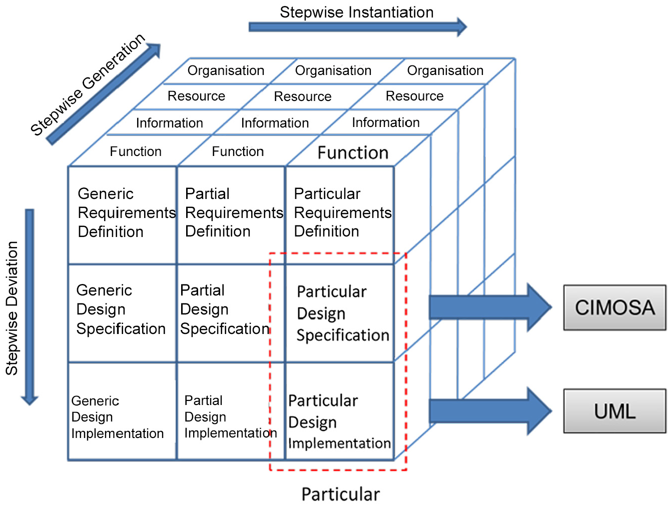
CIMOSA cube showing chosen modelling constructs for design specification and design implementation.

The CIMOSA framework included generic, partial and particular model levels. Models created at the generic level can be applied and re-used for different performance monitoring systems, which require data acquisition, data analysis, data storage and feedback capabilities, contributing towards standardisation of the approach. The partial model in the sports domain would refer to ‘an athlete performance monitoring system’, which extends the concept of generic monitoring models into the sporting domain. This domain requires that the system must also be able to support parameters and processes specific to the training strategy, which must be adaptable based on value judgement of the athlete’s progress (e.g. by performance coaches). The research outlined in this paper is focused on detailing the particular design specification and particular design deployment levels. The following section documents the particular design specification for this system using the CIMOSA methodology. The particular instantiation in a S&C implementation refers to ‘an athlete performance monitoring system within the strength and conditioning domain’. This particular level documents the specific data acquisition technologies, signal processing techniques and feedback mechanisms relevant to the S&C domain (e.g. IMU, CMJ).

System design and deployment using framework

The design specification was guided by the user requirements, identified through consultation with an elite S&C coach and three athletes. The specification is presented, followed by the validation of the selected data acquisition units contributing to both the need for a framework to standardise the development of monitoring systems for CMJ and validation of the hardware used to record the relevant data. An overview of the system is shown Figure 3. The system was comprised of two adjacent tri-axial force platforms to measure bilateral ground reaction forces, as well as a network of wireless IMUs to measure body segment and bar rotation. The force platform was a bespoke solution, which used eight Kistler 9602A piezoelectric transducers, and the wireless IMUs were developed at Loughborough University (for further detail see the research by Le Sage et al.¹⁰). The system was developed to support S&C coaches at the university when analysing jump performance for athletes.

Figure 3.

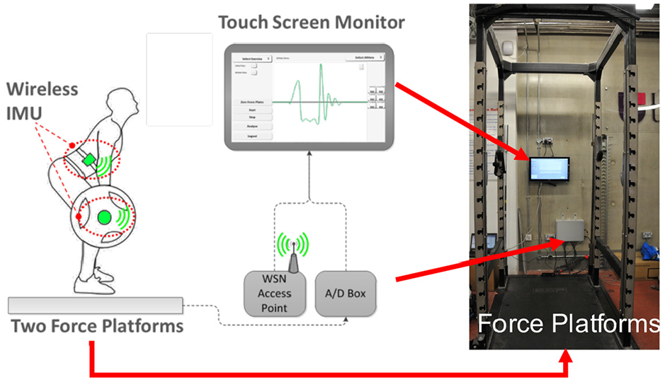
Overview of system components for monitoring performance, WSN is the wireless sensor network, A/D Box converts the analogue signal to a digital signal.

Stakeholder requirements

The design of the system was guided by the requirements of the stakeholders. The stakeholders comprised one S&C coach who utilised the system to monitor performance and three trained athletes from sprinting and high jump backgrounds, each performing 20 CMJs. The coach required that the system improve set-up time for analysis of jump data acquisition for a new exercise with the current manual processes requiring 2 days. Additionally, the coach required that analysis of jump data be completed within 2 s to provide ‘real-time’ feedback. To ensure data privacy, the system must require a secure user log in via user ID and password to allow access. Training strategy and value judgement were not included in the design specification, as they were considered to require bespoke domain expertise provided in confidence by the coach to the athlete.

Context diagram

The particular level Context Diagram highlights six CIMOSA domains. A summary of the interrelated domains is illustrated in Figure 4. The first domain in the Athlete Monitoring System is the Training Strategy (DP1). The Training Strategy domain determines how an athlete transitions from his current state to a point where he can achieve a set of goals typically generated by the coach with input from the athlete.¹¹ The second domain (DP2) is Data Acquisition. This is where quantitative data are captured pertaining to the athlete’s performance. In the S&C domain, this information can be specific to a training session (i.e. number of sets, number of reps or weight lifted) or specific to an exercise (i.e. jump height, peak power or peak force).¹² Technology specific to the S&C domain was highlighted at this stage (i.e. force platforms, wireless IMU and LPTs.^2,13

Figure 4.

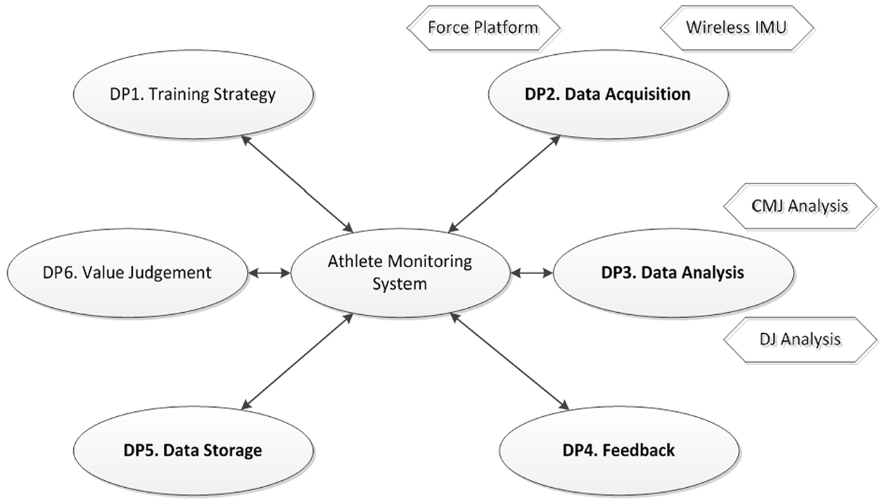
Context diagram for particular level athlete monitoring system.

The third domain is Data Analysis (DP3). Once the raw data have been captured, they must be processed into meaningful, useful information, which can be used to make decisions on athlete performance.¹⁴ Although data analysis is exercise and technology specific, certain aspects of the analysis processes can be shared by similar exercises. Feedback is identified as the fourth domain (DP4), which relates to how the information is selected and displayed to the range of stakeholders (e.g. S&C coach, coach, athlete or system developer). Data Storage is the fifth domain (DP5). In this research, analysed data were stored in a centralised database, whilst raw data were saved to a comma-separated variable (CSV) file located on a local hard drive to enable coaches to utilise pre-determined analysis algorithms and preferred software (e.g. Microsoft Excel). Value Judgement is identified as the sixth domain (DP6). Value Judgement supports the process of using domain knowledge to interpret information provided by the system. For example, an experienced coach could use the gathered information to make decisions on athletes’ performances and adjust training strategies appropriately.¹⁴ Domain processes DP2, DP3, DP4 and DP5 have been the main focus of this research. DP1 and DP6 are heavily reliant on the athlete-coach relationship and are not explored within this research, as the stakeholders involved in the implementation wanted to preserve this relationship and privacy.

Interaction diagram

The second level of decomposition in the CIMOSA is an Interaction Diagram shown in Figure 5, highlighting how the four domains that are the focus of this research (i.e. DP2, DP3, DP4 and DP5) exchange information and utilise resources. The CIMOSA Interaction Diagram enables the flow of information and resources across the domains in the system to be documented. Central to the system designed in this work is a common database, which is shared by all domains. The coach creates a training strategy based on information from value judgement. The athlete carries out the training strategy. Throughout the training strategy, the athlete is monitored through data acquisition. Data are captured through various sensor hardware components (e.g. force plate, IMU). The raw data are then analysed to extract meaningful information. This information is stored in the common database. The information is then fed-back to the coach via a graphical user interface (GUI). This allows the coach to use expert domain knowledge to enact value judgement on the athlete’s progress and adjust the training strategy where appropriate.

Figure 5.

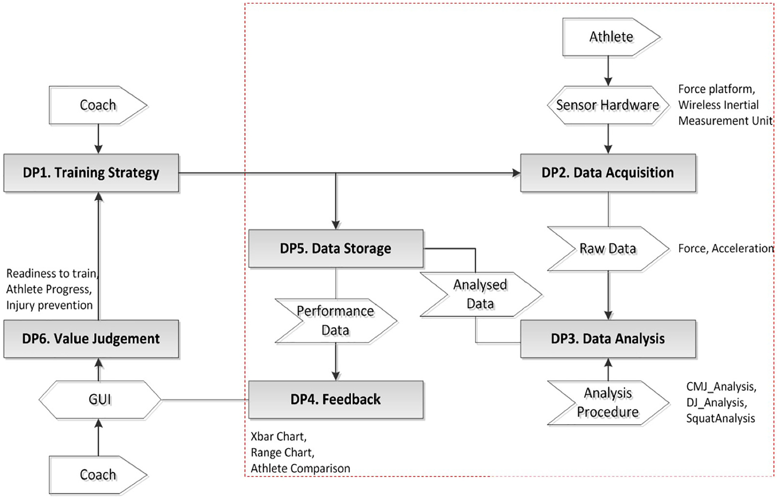
CIMOSA interaction diagram for athlete monitoring system – the dashed line around data storage, acquisition, feedback and analysis is used to highlight the areas of focus for this research.

Structure diagram

The third layer of decomposition is documented using the Structure Diagram (Figure 6). The Structure Diagram is used to identify the structure of the core processes and activities that characterise each domain. The domains are first divided into Business Processes (BPs), before being further decomposed into Enterprise Activities (EAs), which are the fundamental activities within the domain. The Structure Diagram shows the four domains-of-interest (i.e. data acquisition (DP2), data analysis (DP3), feedback (DP4) and data storage (DP5)).

Figure 6.

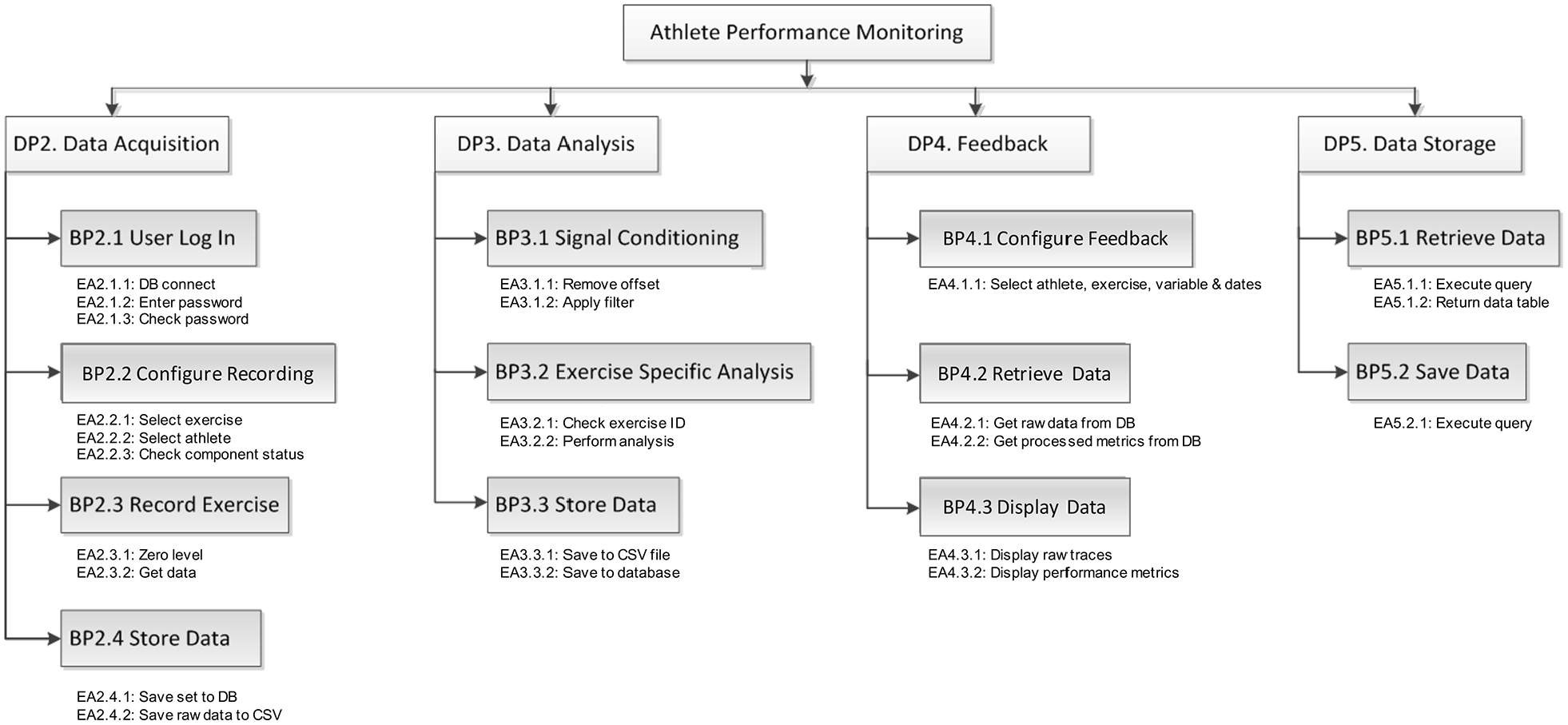
CIMOSA structure diagram for athlete monitoring system.

Domain process 2 (DP2) is comprised of four business processes. Before acquiring data, a user must log into the system (User Log In: BP2.1). This was a requirement from the stakeholder. Specific enterprise activities associated with this include connecting to the database (DB connect: EA2.1.1) and a user credential check (Enter password: EA2.1.2, Check password: EA2.1.3). If the password is not valid, the user is notified and the system remains in the log in state. If the password is valid, the system moves to Configure Recording: BP2.2, where the user must configure the system for recording. The user must select an exercise (Select exercise: EA2.2.1) and select an athlete (Select athlete: EA2.2.2). The system performs a check to verify component status (Check component status: EA2.2.3). Once the system configuration is complete, the user can record an exercise (Record Exercise: BP2.3). The system zeroes the output levels on the force platforms to remove any associated drift of output levels with time that is an inherent feature of piezoelectric force transducers¹⁵ (Zero level: EA2.3.1), before commencing the recording (Get data: EA2.3.2). Finally the system must store the data (Store Data: BP2.4). This is comprised of two enterprise activities. The ‘set’ information (i.e. information regarding the athlete ID, time of recording, exercise ID) is saved to the database (Save set to DB: EA 2.4.1). Then, the raw force data are saved to a comma separated variable ‘.csv’ file (Save raw data to CSV: EA2.4.2).

Domain process 3 (Data Analysis: DP3) is concerned with the determination of performance related parameters from the ground reaction force data in real-time. This process has been decomposed into three business processes: Signal Conditioning: BP3.1, Exercise Specific Analysis: BP3.2 and data storage (Store Data: BP3.3). Signal Conditioning has been broken down into two EAs. The data must first be zeroed due to small continual drift of a piezoelectric output voltage under pressure¹⁵ (Remove offset: EA3.1.1) before a digital filter is applied (Apply filter: EA3.1.2) to reduce the level of random noise within the signal. At this point, an exercise specific analysis is performed (BP3.2). This EA extracts useful information in the form of pre-determined parameters (specified by the stakeholders and best practices within the S&C domain) from the raw data. The final business process in DP3 is data storage. The processed parameters are stored to a ‘.csv’ document (Save to CSV file: EA3.3.1), before being stored in a database (Save to database: EA3.3.2). The parameters are stored in a ‘.csv’ document at the request of the stakeholders, whilst the storage in a database enables the system to manage the data.

Domain process 4 is divided into three business processes: feedback configuration (Configure Feedback: BP4.1), data retrieval (Retrieve Data: BP4.2) and data display (Display Data: BP4.3). To configure the feedback settings, the user must select an athlete, exercise, performance variable and date or range of dates. BP4.2 (Retrieve Data) then uses this information to retrieve raw data (Get raw data from DB: EA4.2.1) and processed data (Get processed metrics from DB: EA4.2.2). The BP4.3 (Display Data) displays the data in graphical (Display raw traces: EA4.3.1) and tabular (Display performance metrics: EA4.3.2) forms.

The final domain is DP5, Data Storage. This is divided into two business processes: data retrieval (Retrieve Data: BP5.1) and data storage (Save Data: BP5.2). These business processes are used by the other domains in order to save and access data when required.

Activity diagram

The final diagrams in the CIMOSA decomposition are Activity Diagrams. These are used to document the sequential flow of data, associated resource utilisation and functionality for each of the domain processes. These low-level diagrams provide detailed procedural information about each of the processes. Figure 7 shows the Activity Diagram for DP2, Data Acquisition. GUI screens have been added to the diagram to aid visualisation of how the system is presented to the stakeholders at each point in the sequence of activities. BP2.1 (User Log In), BP2.3 (Record Exercise) and BP2.4 (Store Data) all require the system to interact with the database. All data storage and retrieval tasks are managed through DP5, Data Storage. Thus, each of these processes requires communication with DP5. BP2.3 (Record Exercise) also requires interaction with hardware components linked to the core sensing elements. This is carried out through an application program interface (API).

Figure 7.

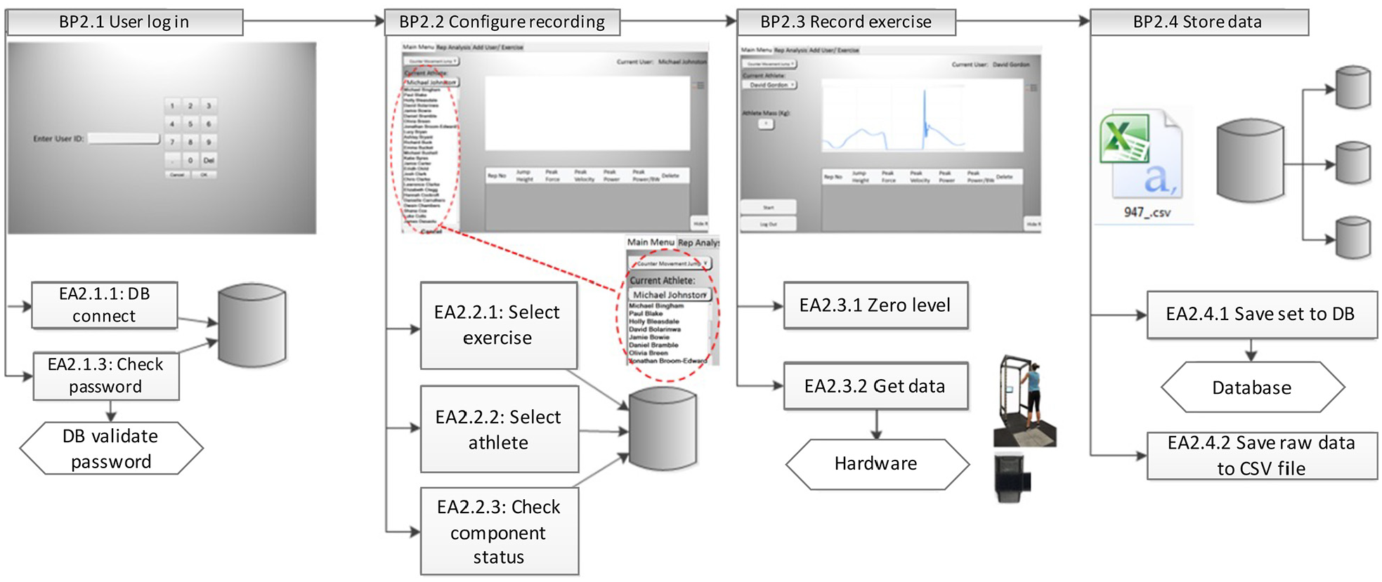
Activity diagram for DP2, data acquisition.

Implementation view and particular design

The following section documents the Particular Design deployment. The Particular Design deployment has been represented using UML Class and Sequence diagrams. The implementation view demonstrates how the particular design specification is to be executed. UML class diagrams are used to document the static structure of the system, whilst UML sequence diagrams show the program flow and the interaction between classes. A layered architecture is utilised to separate the business layer from the application layer. Figure 8 shows the composition of these two layers.

Figure 8.

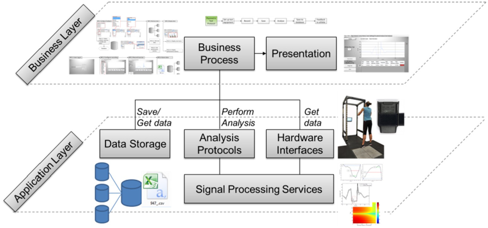
Distinction of business and application layers.

The Business Layer is composed of the Business Processes and Presentation (i.e. GUI). The Application Layer is composed of the Data Storage, Analysis Protocols, Hardware Interfaces and Signal Processing Services. This architecture ensures that the business processes can be designed, implemented and adapted regardless of system hardware and the methods used to record, analyse and store the data. This is particularly useful as it is easily adaptable for other applications. Figure 9 is a Class Diagram showing how the layered architecture has been implemented.

Figure 9.

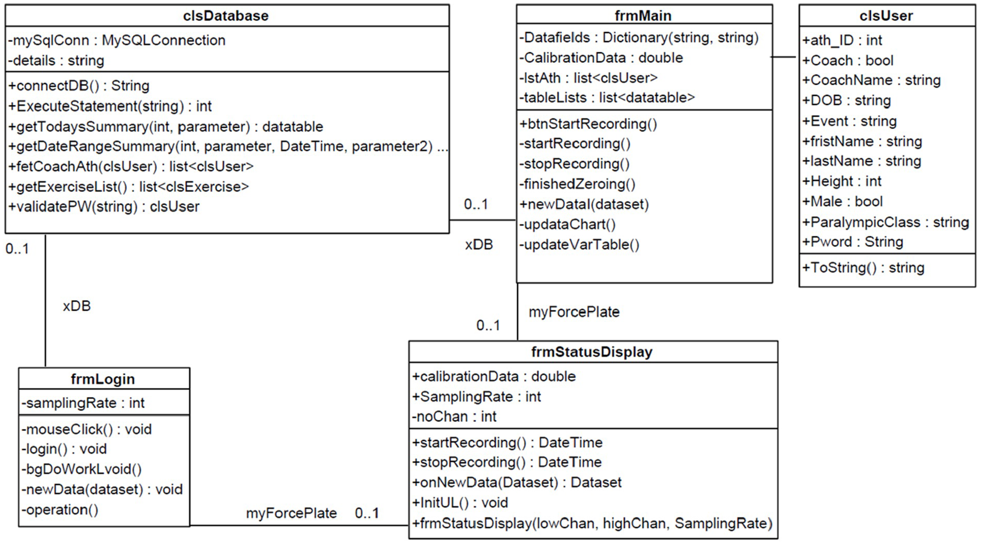
UML class diagram showing log in and main form classes.

The Business Layer is comprised of two classes: ‘frmLogin’ and ‘frmMain’. The start-up object for the application is ‘frmLogin’, which handles the user log in process. This form has two associations, a database manager (clsDatabase) and a hardware interface (frmStatusDisplay). The core processing and interface operations are performed by ‘frmMain’. This form has three associations: a database manager (clsDatabase), a hardware interface for the force platform (frmStatusDisplay) and a list of available users (clsUser). This class contains methods which carry out the business processes. The core classes have been shown for ease of interpretation. Incoming data are handled by ‘newData’, which stores data in temporary memory under the ‘datafields’ attribute. The method ‘btnStartRecording’ prepares the system for a new recording and ‘startRecording’ initiates data flow from each of the hardware applications. To stop a recording, ‘stopRecording’ is called either when the user manually presses the stop or cancel button or if the allocated time has elapsed (typically 8 s). This method calls the appropriate analysis service from the ‘analysisProtocols’ on the application layer and communicates with the data storage manager to save the analysed parameters. Figure 10 is a Class Diagram showing the composition of the analysis services, focusing on the CMJ and drop jump (DJ) exercises. Each exercise is composed of one ‘process’ class (e.g. clsCMJProcess), a ‘major’ parameter class (e.g. clsBilateralCMJ) and a ‘minor’ parameter class (clsCMJParameters).

Figure 10.

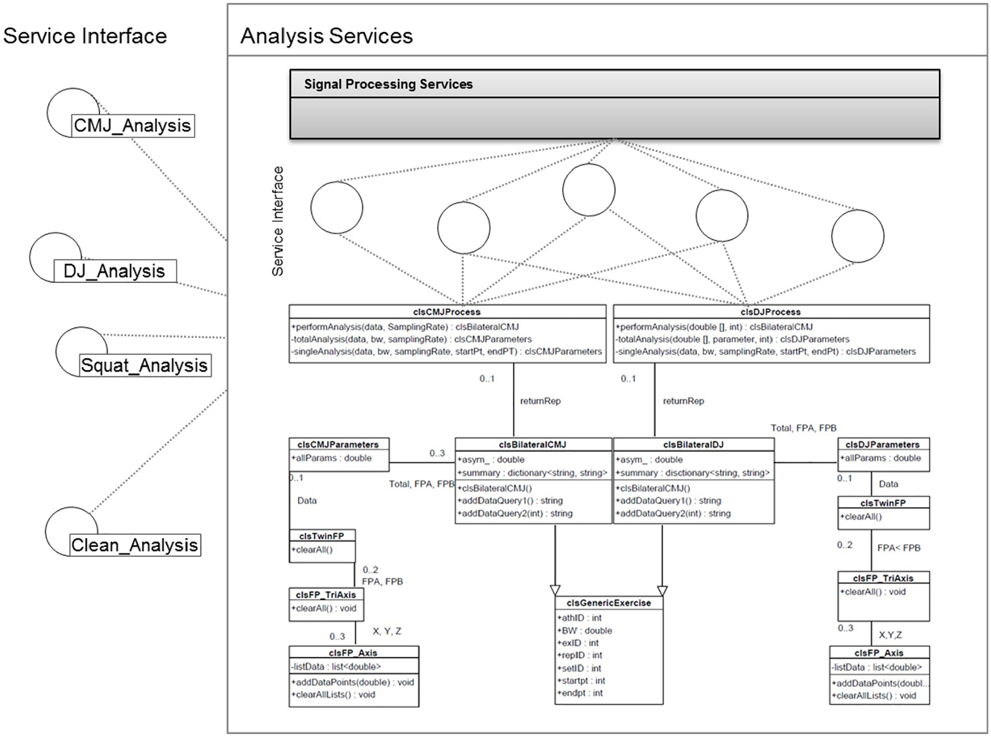
UML class diagram showing analysis classes.

The minor parameter class contains parameters which are common across the Total, FPA and FPB analysis. The minor parameter class has one association (‘clsTwinFP’). This class contains two ‘clsFP_TriAxis’ classes (FPA and FPB), which in turn each contain three ‘clsFP_Axis’ axes (i.e. X, Y and Z). A clsFP_Axis class contains data which are common across all axes of force measurement (i.e. force, resolved force, velocity, displacement, power and impulse).

The major parameter class contains three minor parameters classes as associations (‘Total’, ‘FPA’ and ‘FPB’). This class also holds any parameters which describe asymmetry (e.g. asymmetric force, asymmetric impulse). There are three methods in the major parameter class including a default constructor and two database query builders. The first query builder generates a query to save the asymmetric parameters, whilst the second builds a query to save the Total, FPA and FPB parameters. This arrangement ensures a loose coupling between the database manager and analysis classes, which promotes re-use. The process class has the major parameter class as an association. This enables the process class to populate the parameter class with analysed performance metrics. The process class has one public method (‘performAnalysis’). The inputs to this method are the GRF data from FPA and FPB and the sampling rate. This method encapsulates the business logic required to perform the exercise specific analysis. The signal processing services class contains processes which are common to several exercises. These should be re-used where possible to reduce development overhead when defining new processes. The public method ‘performAnalysis’ outputs a corresponding major parameter object (clsBilateralCMJ in this case). Figure 11 is a Sequence Diagram showing BP2.2 (Configure Recording), BP2.3 (Record Exercise) and BP2.4 (Store Data).

Figure 11.

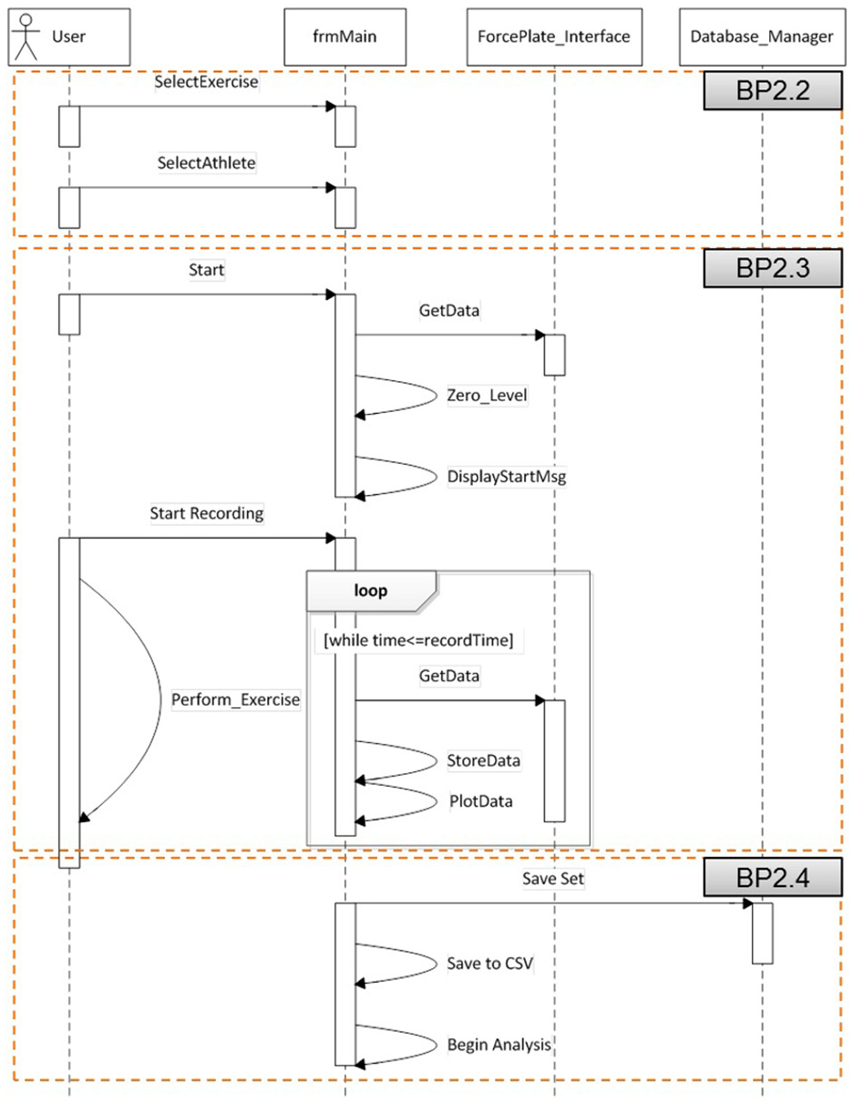
UML sequence diagram showing data acquisition process, highlighting the association with pre-defined CIMOSA business processes (see Figure 7).

Data acquisition process

The user must first configure the system by selecting an athlete and exercise. The user then presses a start button to begin the recording process (BP2.3). The ‘frmMain’ class starts the flow of data by calling the ‘GetData’ method of the ‘ForcePlate_Interface’ class. Data are then sent to the ‘frmMain’ class. The force outputs are zeroed by averaging the data for 1 s and removing this bias from the rest of the data. Piezoelectric force transducers are subject to a temporal drift, hence zeroing the force platforms before recording ensures the effect of this drift is minimised (approximately 0.04 Ns⁻¹ for Kistler 9602 transducers following the manufacturer’s recommended procedure¹⁶). Once the offset has been calculated, the system prompts the user with a start message. The user presses ‘Start Recording’ and performs the exercise. The ‘frmmain’ class interrogates the ForcePlate_Interface with the ‘GetData’ method. The data are stored locally and plotted, until a pre-set time has passed. Once the pre-set time has elapsed, the system begins BP2.4, where the ‘frmMain’ class interacts with the ‘Database_Manager’ class to save the data. The system begins the analysis process immediately after the recording has taken place. This ensures that the analysis is performed within the 2 s limit for acceptable ‘real-time’ analysis as requested by the stakeholder (coach) and that the data must be analysed according to an exercise-specific protocol (BP3.2). Figure 12 shows a typical countermovement force and velocity trace, as well as examples of the software code (in Visual C++), used to derive a range of temporal features. The algorithms are modified versions of the functionalities outlined as best practice by Street et al.¹⁷ and Baca.¹⁸

Figure 12.

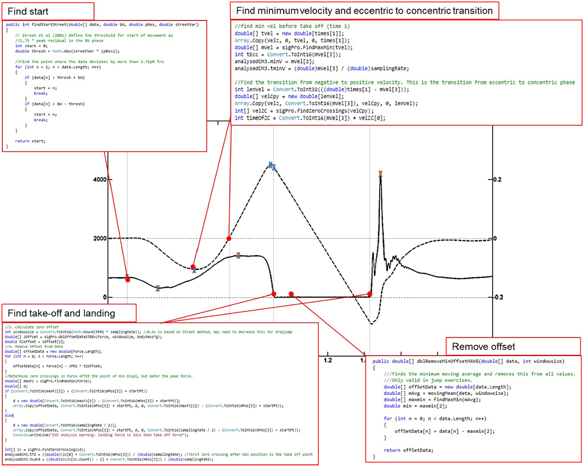
Typical CMJ force and velocity trace showing code snippets used to extract the start, take-off and landing points, minimum velocity and eccentric to concentric transition point.

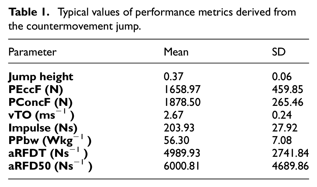
When defining services, it is important to understand how the granularity can affect program efficiency and re-use, designing a suitable service which is likely to be reused, for example a focused service.¹⁹ The temporal features are the fundamental features which must be extracted before performance metrics can be derived. Some temporal features, such as the start and end points, take-off and landing, are generic for a wide range of exercises. Some features, such as the eccentric to concentric transition, are specific to the CMJ exercise. Typical values for the parameters derived from this process have been given in Table 1.

Table 1.

Typical values of performance metrics derived from the countermovement jump.

Parameter	Mean	SD
Jump height	0.37	0.06
PEccF (N)	1658.97	459.85
PConcF (N)	1878.50	265.46
vTO (ms ⁻¹ )	2.67	0.24
Impulse (Ns)	203.93	27.92
PPbw (Wkg ⁻¹ )	56.30	7.08
aRFDT (Ns ⁻¹ )	4989.93	2741.84
aRFD50 (Ns ⁻¹ )	6000.81	4689.86

The first operation in a jump exercise is to remove any offset in the data. The offset is defined as the minimum value in a 0.35 s moving average performed throughout the dataset. The offset is then removed from all points in that trial. The start of the exercise is determined as the first point in the force trace that deviates from body weight (BW) by a set threshold. The threshold has been defined as 1.75 times the peak residual force observed within the stationary 2 s of data at the start of the trial as specified by Street et al.¹⁷ The take-off and landing points are similarly determined using a threshold. This threshold is set at 1.75 times the peak residual in the 0.35 minimum moving average period. Repeated trials showed that several athletes un-weighted the platform during the countermovement. As a result, the take-off and landing points could be wrongly classified. To avoid this error, the force trace was automatically cropped from the point of minimum displacement (i.e. the bottom of the countermovement) to the end of the trial. The point of minimum velocity is defined as the smallest observed velocity before the take-off time. The eccentric to concentric transition is defined as the first zero crossing in velocity after the point of minimum velocity. Analysis processes, which are generic across a range of exercises, have been grouped into a class of signal processing services. Figure 13 shows the CMJ and DJ sequence diagrams, showing the interactions with the generic signal processing services.

Figure 13.

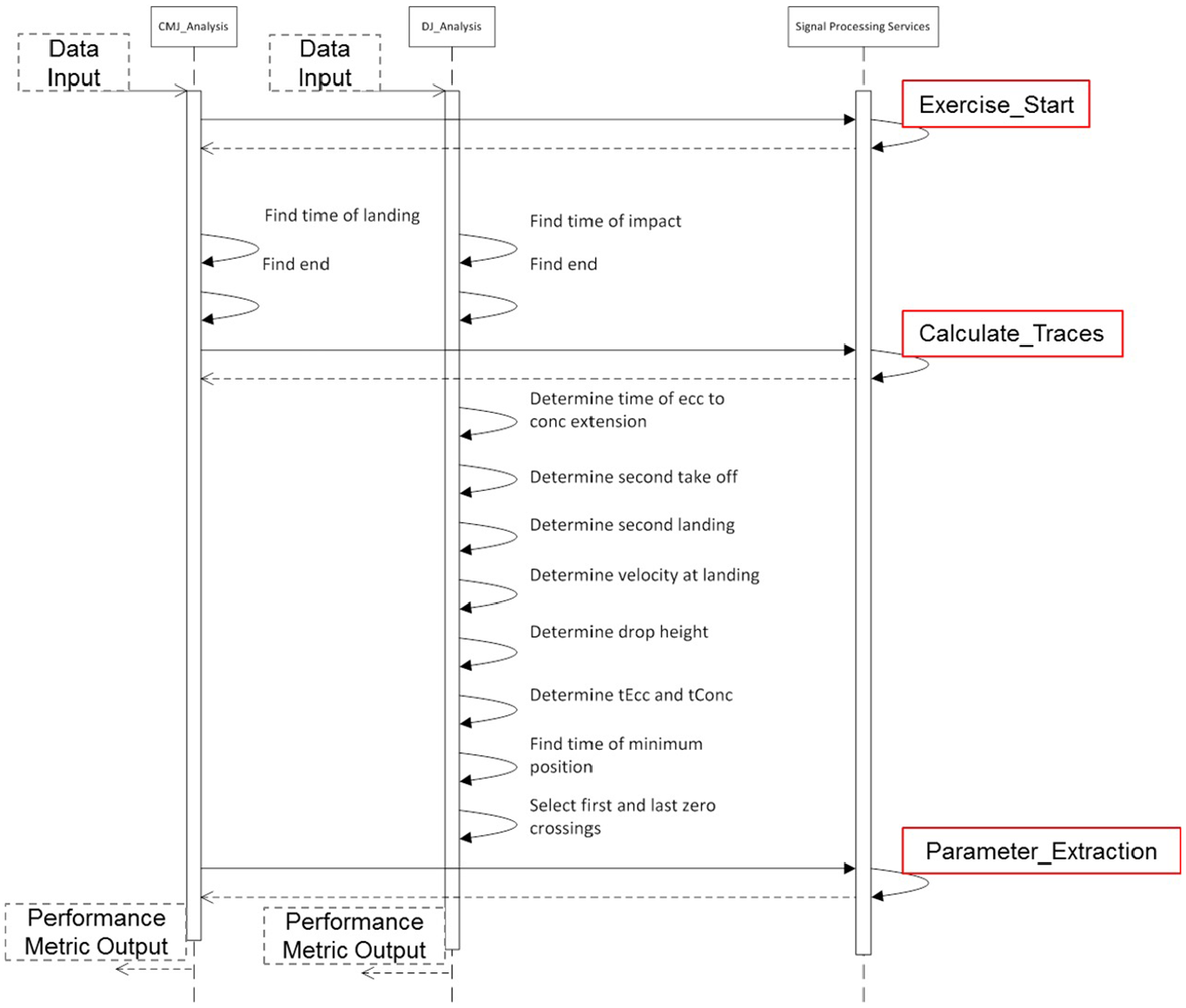
Analysis process showing signal processing services.

Validation of the system

Validation of user requirements

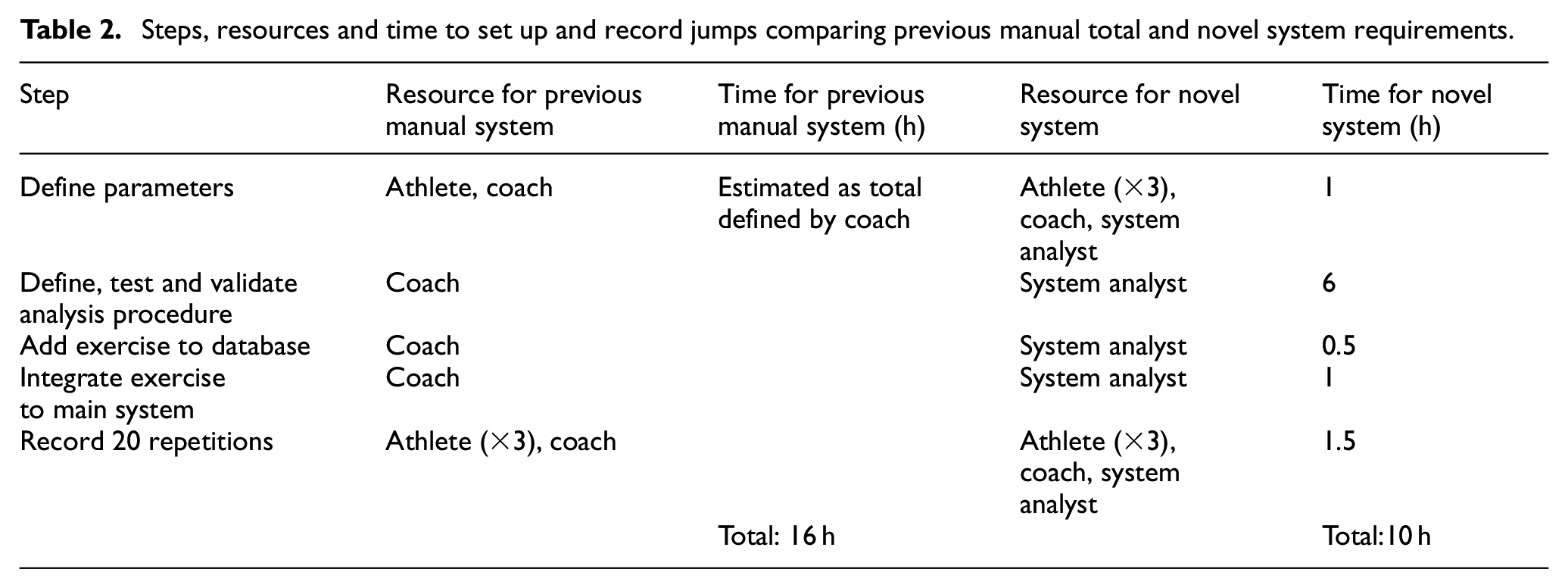
The primary requirement specified by the coach (identified as the primary end user for the system) was that the process for setting up recording of a new jump activity should be quicker than the existing manual process. The new system required 10 h in total (recorded during use of the system for three athletes performing 20 jumps each). Although the system reduced the time taken to set up and record a new jump, the novel system required the addition of a system analyst to support set up and trouble shooting. Additionally, the novel system could support remote set up and integration of exercises into a database, reducing the requirement for manual work by the coach. A comparison of the resource and time for the previous manual system and the novel system is shown in Table 2.

Table 2.

Steps, resources and time to set up and record jumps comparing previous manual total and novel system requirements.

Step	Resource for previous manual system	Time for previous manual system (h)	Resource for novel system	Time for novel system (h)
Define parameters	Athlete, coach	Estimated as total defined by coach	Athlete (×3), coach, system analyst	1
Define, test and validate analysis procedure	Coach		System analyst	6
Add exercise to database	Coach		System analyst	0.5
Integrate exercise to main system	Coach		System analyst	1
Record 20 repetitions	Athlete (×3), coach		Athlete (×3), coach, system analyst	1.5
		Total: 16 h		Total:10 h

Validation of hardware

The hardware adopted for use in the CIMOSA/UML framework system were validated to demonstrate their use in a S&C setting. The IMU modules comprise accelerometers and gyroscopes to record acceleration and give raw outputs from A/D converters.²⁰ IMU recordings are subject to drift of the sensitivity and offset, causing the need to be calibrated.²¹ Calibration for inertial sensors generally compares the raw sensor output to a known quantity from physical phenomenon generated by calibration set ups and instruments.²⁰ One such method is to apply gravitational acceleration twice to each axis of the device to determine the coefficients of calibration for the specific IMU.²¹ When static, the accelerometers will measure the vertical gravity vector. Each sensing axis can be subjected to +9.81, 0 and −9.81 ms⁻² by a sequence of orientations with respect to the gravity vector, while the six-position and angular rate tests were used to calibrate the accelerometers and gyroscopes used in the study.^22,23 An example output for Z-axis calibration and the corresponding linear regression output model are shown in Figure 14.

Figure 14.

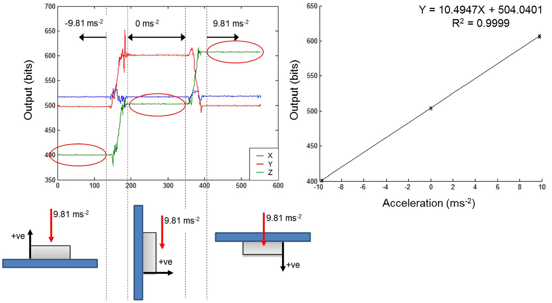
WSN accelerometer calibration.

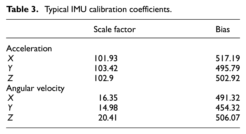
To calibrate the gyroscope, a Haas TL2 lathe was used to subject each axis to a range of angular velocities.²⁴ Each unit was rotated through a range of ±180 RPM in increments of 30 RPM. According to the manufacturer (Haas), angular velocity is accurate to within ±0.125% of the selected speed. Angular velocity of the lathe was confirmed by checking against the period of the accelerometer waveform. At the slowest speed (30 RPM), the period of the lathe was 2.0000 ± 0.0025 s. The sampling rate of the accelerometer was 50 Hz, giving a temporal resolution of 0.02 s. This method proved the period of the lathe was correct to within ±0.02 s for all angular velocities. Since the lathe had a higher timing resolution than the accelerometer, the selected speeds from the lathe were used to represent the angular velocities. Typical calibration coefficients for an inertial measurement unit used in this research are summarised in Table 3.

Table 3.

Typical IMU calibration coefficients.

	Scale factor	Bias
Acceleration
X	101.93	517.19
Y	103.42	495.79
Z	102.9	502.92
Angular velocity
X	16.35	491.32
Y	14.98	454.32
Z	20.41	506.07

A Vicon motion capture system²⁵ was used as a ‘gold standard’ reference to track the motion of the IMU.^1,26 Four retro-reflective markers were placed on the body of the IMU, as shown in Figure 15(a). The Vicon system recorded the position of the four markers in 3D space with a sampling rate of 200 Hz. The IMU recorded data at a rate of 50 Hz. The centroid of the four markers was used as a reference for the IMU motion. Vicon displacement data were differentiated twice with respect to time to obtain velocity and acceleration. A fourth order low pass filter was used to reduce noise introduced through each differentiation, a cut-off frequency of 14 Hz was selected using the residual analysis technique.²⁷

Figure 15.

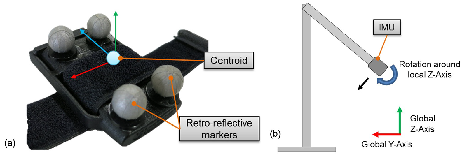
(a) Inertial measurement unit with retro-reflective markers and approximate location of centroid and (b) experimental set up and designation of global axis for pendulum trials.

Pendulum trial

In the first experiment, a pendulum was used to record a set of repeatable, predictable trials which would induce acceleration in two axes. Following this, a set of five CMJ were performed, as this is a common test used in the S&C domain to determine explosive strength, readiness to train and fatigue.² Figure 15(b) shows the experimental setup for the pendulum trials. The pendulum arm was 45 cm long and attached to a pivot via a ball bearing to reduce friction. The IMU was attached to the pendulum at a distance of 35 cm from the pivot centre. The IMU was oriented so that the major axis of rotation was around the local Z-axis of the IMU, whilst the major displacements were in the global Y and Z axes. The pendulum arm was raised to approximately 90° and released. The arm was left to swing until it came to rest and data were synchronised using an external trigger.

A series of five trials were performed. Figure 16 shows a comparison of typical IMU and Vicon outputs for the pendulum trials.

Figure 16.

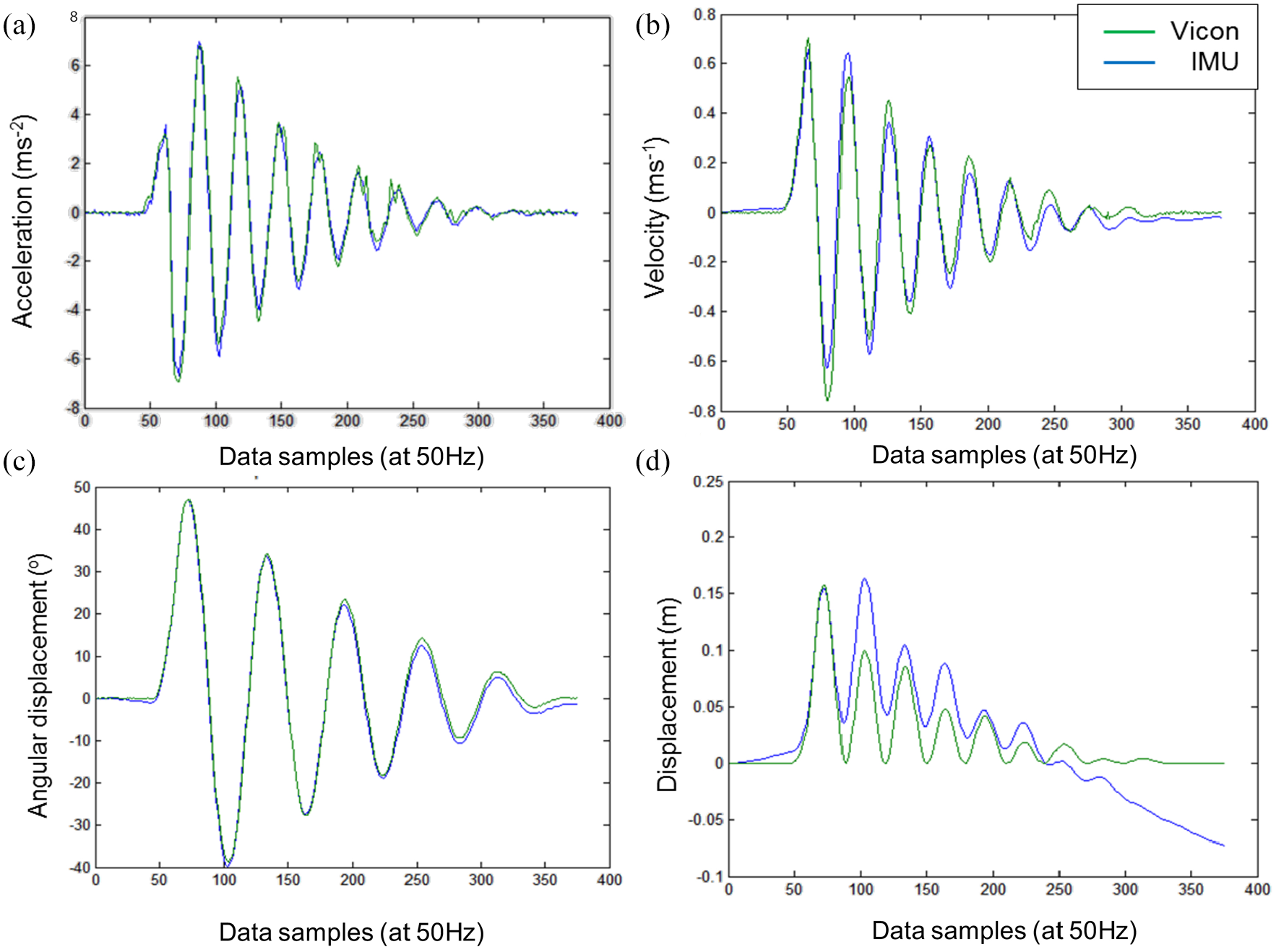
Comparison of Vicon and IMU measurements in the Z-axis for: (a) acceleration, (b) velocity, (c) angular displacement and (d) displacement.

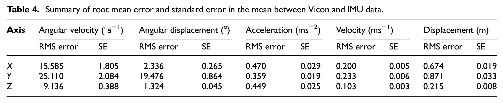
The pendulum took approximately 6 s to come to rest following release. For each trial, the root mean square (RMS) error and standard error in the mean (SE) were calculated and averaged. These results are summarised in Table 4.

Table 4.

Summary of root mean error and standard error in the mean between Vicon and IMU data.

Axis	Angular velocity (°s⁻¹)		Angular displacement (^o)		Acceleration (ms⁻²)		Velocity (ms⁻¹)		Displacement (m)
Axis	RMS error	SE	RMS error	SE	RMS error	SE	RMS error	SE	RMS error	SE
X	15.585	1.805	2.336	0.265	0.470	0.029	0.200	0.005	0.674	0.019
Y	25.110	2.084	19.476	0.864	0.359	0.019	0.233	0.006	0.871	0.033
Z	9.136	0.388	1.324	0.045	0.449	0.025	0.103	0.003	0.215	0.008

A linear regression model was used to compare the two traces. The coefficient of determination (R²) for each variable is shown in Table 5.

Table 5.

Summary of coefficient of determination (R²) from linear regression model comparing Vicon and IMU data.

Axis	Angular velocity	Angular displacement	Acceleration	Velocity	Displacement
X	0.129	0.235	0.169	0.026	0.025
Y	0.042	0.385	0.987	0.955	0.077
Z	0.990	0.998	0.969	0.951	0.563

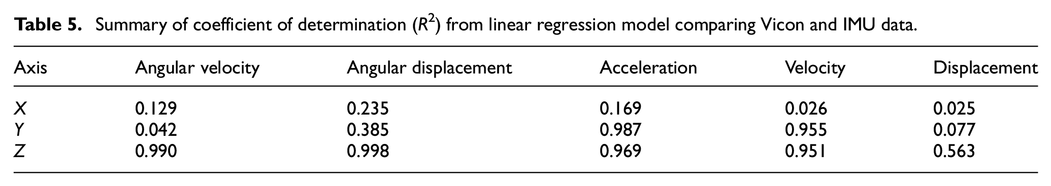
Angular velocity showed a high coefficient of determination for rotations around the Z-axis (R² = 0.99, p = 0.01), however this was lower for rotation around the X- and Y-axes. The major rotation in this set of trials was around the Z-axis. Rotation around the X- and Y-axes were constrained by the pendulum; hence the measured output was primarily noise. This could explain the low coefficient of determination on the X- and Y-axes. Similarly, RMS error for rotations around the Z-axis was lower than those around the X- and Y-axes (9.14 compared to 15.59 and 25.11). Angular displacement for the IMU was determined through integration of the angular velocity and was measured by the gyroscope. The IMU angular displacement can be seen to drift (Figure 16), resulting in an increase in error towards the end of the trial. Vicon determines angular displacement by computing the arctan of the opposite and adjacent position vectors and is not subject to drift. RMS error in the Z-axis was 1.324°, which is in line with what has been reported in literature.²² Coefficient of determination in the Z-axis was high, showing a good level of agreement between the two methods (R² = 0.998, p = 0.01). RMS error in the X- and Y-axes were 2.33° and 19.5°, respectively. Since rotation was constrained in these two axes, this error was likely to be caused by drift in the signal. There is very little difference when visually comparing the two acceleration traces (Figure 16). The Vicon trace was differentiated twice to obtain acceleration. This introduces noise in the signal and a low pass filter was used to remove this (method used by Winter²⁷). The coefficient of determination for both the Y- and Z-axes were high (R² = 0.987 and 0.969, respectively, with p = 0.05). This was as expected as the major acceleration occurs in these two axes. RMS errors in X-, Y- and Z-axes were similar with values of 0.47, 0.36 and 0.45 ms⁻², respectively. Coefficient of determination for velocity was high for the Y- and Z-axes (R² = 0.955 and 0.951, respectively, with p = 0.05). The RMS error was lower for velocity in the Z-axis (0.1 ms⁻¹), compared with the X- and Y-axis (0.2 and 0.23 ms⁻¹, respectively). This was as expected as error is introduced into the IMU signal through integration. The error in the IMU increased when comparing displacement measurements. Coefficient of determination was low for all axes and the RMS errors were high. This increase in error was due to a propagation of errors due to integration of small offsets within the velocity trace.

CMJ trial

For the CMJ trials, the IMU was placed on the athlete’s lower torso, at the approximate location of the T12 vertebrae (the thoracic vertebrae which is located in line with the base of the ribcage). In this trial, the major movement was in the Z- and X-axes, whilst angular rotation occurred primarily around the Y-axis (see Figure 17).

Figure 17.

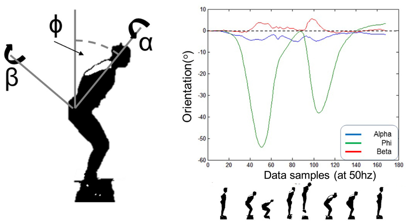
Example IMU rotation measurements recorded using the countermovement jump trial.

Figure 18 shows comparisons of Vicon and IMU angular displacement around the Y-axis and velocity traces in the Z-axis for a CMJ. The CMJ trial was approximately 3.5 s long, which was shorter than the typical length of a pendulum trial (6 s). However, a drift in velocity was observed across all countermovement jump trials determined from the IMU acceleration integration (see e.g. Figure 18(a) and (c)). The larger error in the CMJ trials compared to the pendulum trials may be the result of the faster movement in the CMJ (i.e. CMJ peak +ve and −ve velocities of 2.7 and 2.8 ms⁻¹ respectively versus the pendulum trial peak +ve and −ve velocities of 0.7 and 0.8 ms⁻¹, respectively).

Figure 18.

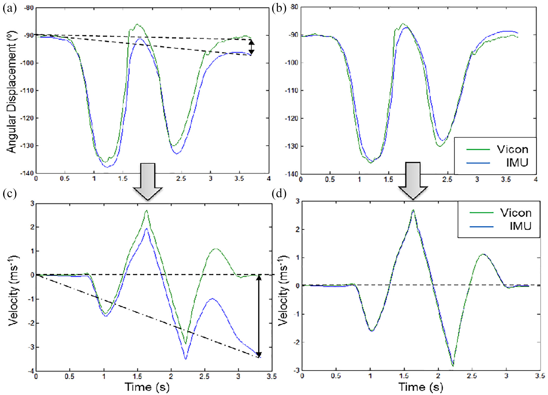
Vicon and IMU outputs for a typical CMJ trial showing: (a) original angular displacement, (b) corrected angular displacement, (c) original velocity and (d) corrected velocity.

The athlete was stationary at the beginning and end of a CMJ trial. Hence, the boundary conditions for the velocity trace were that the velocities at the start and end of the trial were assumed to be zero and were used to remove the drift in the velocity. To determine boundary conditions for the angular displacement, the orientations at the start and end of the trial were calculated from the accelerometer outputs. Both of these boundary conditions were used to remove any linear gradient from the data using equation (1):

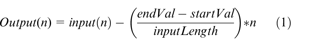
Output (n) = input (n) - (\frac{endVal - startVal}{inputLength}) * n

(1)

In equation (1), ‘endVal’ is the end boundary condition and ‘startVal’ is the starting boundary condition. Figure 18(b) and (d) show the angular displacement and velocity following this correction. Table 6 shows the error in angular displacement, angular velocity, acceleration, velocity and displacement. The RMS error and standard error in the mean have been calculated and averaged across the five trials using:

Method A: un-corrected velocity and orientations

Method B: corrected velocity and orientations

Table 6.

Summary of mean error and standard error between Vicon and IMU data. Method A is without drift correction, method B is with drift correction.

Axis	Angular velocity (°s⁻¹)		Angular displacement (^o)		Acceleration (ms⁻²)		Velocity (ms⁻¹)		Displacement (m)
Axis	Mean error	SE	Mean error	SE	Mean error	SE	Mean error	SE	Mean error	SE
A
X	29.591	1.633	184.519	9.698	4.762	0.434	3.083	0.196	2.746	0.228
Y	25.637	2.221	8.539	0.497	2.352	0.168	2.676	0.167	2.585	0.203
Z	17.386	1.137	0.947	0.054	3.673	0.185	3.503	0.197	3.148	0.252
B
X	24.647	1.585	6.817	0.295	3.166	0.439	0.291	0.027	0.224	0.012
Y	20.910	2.087	2.620	0.164	0.690	0.069	0.229	0.011	0.273	0.013
Z	13.272	1.126	0.883	0.050	0.583	0.079	0.057	0.004	0.047	0.003

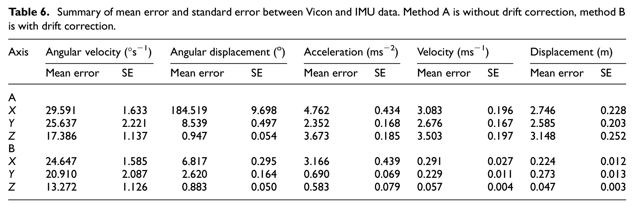
The RMS error was lower for method B (i.e. linear correction algorithm) compared to method A (basic analysis) across all metrics (e.g. by an average of 65% across all metrics). Therefore, where possible, the linear correction algorithm was applied. Similar to the pendulum trial, errors were lowest in the axis of the major movement. It is noted that RMS errors in angular displacement, velocity and position were lower for the CMJ trials (Table 4) than for the pendulum trials (Table 6). However, errors in acceleration and angular velocity were higher in the CMJ than the pendulum trial. A linear regression model was used to enable the Vicon and IMU traces to be compared. The coefficient of determination (R²) for each variable using the two methods is shown in Table 7.

Table 7.

Summary of coefficient of determination (R²) from linear regression model comparing Vicon and IMU data. Method A is without drift correction, method B is with drift correction.

Axis	Angular velocity	Angular displacement	Acceleration	Velocity	Displacement
A
X	0.153	0.335	0.619	0.100	0.135
Y	0.806	0.778	0.127	0.065	0.330
Z	0.424	0.529	0.759	0.647	0.358
B
X	0.198	0.732	0.807	0.646	0.279
Y	0.823	0.973	0.508	0.109	0.247
Z	0.478	0.519	0.967	0.995	0.957

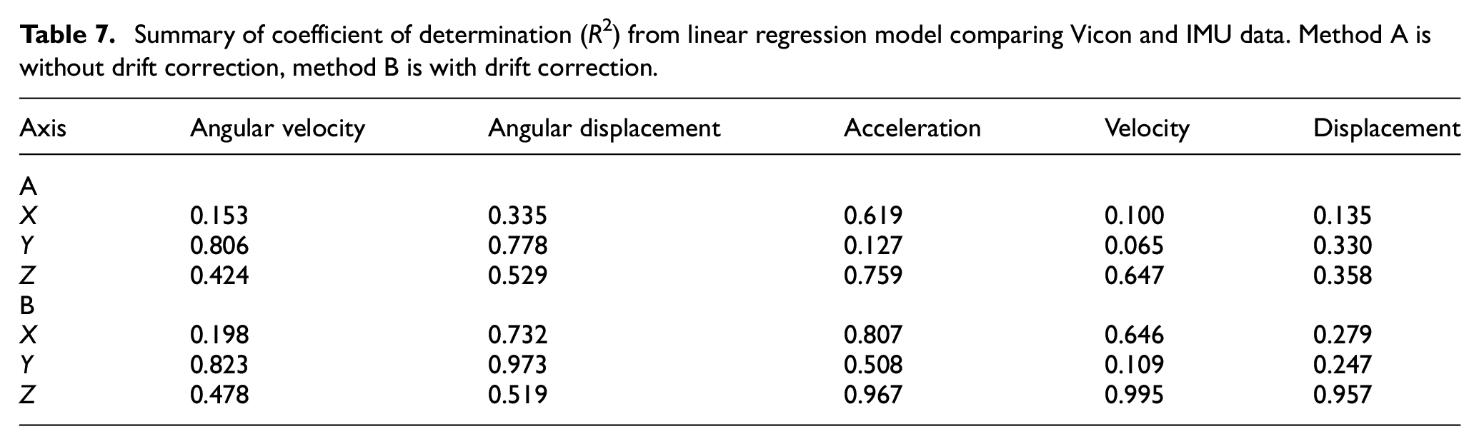
Coefficients of determination were higher for method B (linear correction algorithm) compared to method A (basic analysis). In the Z-axis, acceleration and displacement comparisons showed significance at p = 0.05, whilst the velocity comparison was significant at p = 0.01. Comparison of angular displacement in the Y-axis shows significance at p = 0.05. These results are similar to those of the pendulum trials, indicating that the IMU shows good accuracy (average differences between IMU and Vicon <5%) in the major axes of movement. Based on the results from these preliminary trials, it has been shown that an IMU is able to capture kinematic information to a sufficient degree of accuracy (i.e. >95% in the principal components) for movements that are typical in the S&C domain.

Conclusions, limitations and further work

The aim of the work presented in this paper was to develop a system towards standardising the process of performance monitoring within the S&C domain. Design specification was presented using CIMOSA context, interaction, structure and activity diagrams. Six CIMOSA domains were identified using the Context Diagram. An Interaction Diagram was used to identify the key relationships between the six domains. The domains were decomposed into business processes and enterprise activities using a Structure Diagram. Finally, Activity Diagrams were used to show the sequential flow of key functionalities within chosen domains. Design implementation was achieved through use of UML Class and Sequence Diagrams. A Class Diagram was constructed to show the static structure and organisation of the system. The CIMOSA framework was used as the foundation architecture for system development, however the UML was required to document the design implementation stage in an appropriate amount of detail.

The framework was implemented utilising a wireless IMU^3,10 and validated for use within the S&C domain. The IMU was calibrated using the six-position method and angular rate test.²³ An optical motion capture system was used as a gold standard reference measure to compare acceleration,² velocity, displacement, angular rate and angular displacement of the IMU in two trials. A linear correction algorithm was used to reduce drift and increase the accuracy of the angular displacement, velocity and displacement traces. In the pendulum trial, R² values of 0.951–0.998 were observed in the major axes of movement. In the CMJ trial, R² values of 0.823–0.995 were observed in the major axes of movement. These findings suggest that the IMU can be used to provide a valid measure of performance within the S&C domain.

Limitations of the study include the use of a limited range of hardware (IMU device and force platforms). According to previous studies, such technologies are reliable tools for the assessment of CMJ, however the values obtained do not transfer to other hardware. Future studies should address the range of additional hardware that could be compared to the data presented in this study.² The present implementation of the system required the coach and system analyst to be present to set up and validate the system and input new exercises to the system. Although the system analyst could potentially implement new exercises remotely in the future, the prototype nature of the system required the analyst to be present to troubleshoot and assist with the input of new jump profiles to the system. Future iterations of the system should support end user interaction with the system through the use of tutorials and support documentation with remote assistance provided by the system analyst.

The current implementation requires the system analyst to be present to troubleshoot and recalibrate as needed. Further development is required to improve the robustness of the system and automate the identification and rectification of errors. Proposed future work includes the exploration of machine learning techniques to address these issues and further automate data processing for training insight. Another promising avenue is the use of smart identification of athletes to support automated calibration, as well as the potential for performance profiling and feedback (e.g. using wearable device or identification card containing a radio frequency ID tag).

In summary, the design and evaluation of an appropriate architecture for a system to monitor performance in real time within the S&C domain was presented and validated. A novel system was developed and the hardware was validated, which integrates two tri-axial force platforms (ground force granularity), an IMU and a wireless sensor network, providing increased information to the user and reducing the time required for coaches to capture and analyse data from athlete jump. The system was developed to address the need for standardisation of system development of monitoring systems to support CMJ analysis and the proposed architecture can be adapted for further development of standardised athlete monitoring systems in the future.

Footnotes

Declaration of conflicting interests

The author(s) declared no potential conflicts of interest with respect to the research, authorship, and/or publication of this article.

Funding

The author(s) received no financial support for the research, authorship, and/or publication of this article.

ORCID iDs

Katherine van Lopik

Steven Hayward

References

Petrigna

Karsten

Marcolin

, et al. A review of countermovement and squat jump testing methods in the context of public health examination in adolescence: reliability and feasibility of current testing procedures. Front Physiol 2019; 10: 1384.

Ferro

Floría

Villacieros

, et al. Maximum velocity during loaded countermovement jumps obtained with an accelerometer, linear encoder and force platform: a comparison of technologies. J Biomech 2019; 95: 109281.

Chakravorti

Le Sage

Slawson

, et al. Design and implementation of an integrated performance monitoring tool for swimming to extract stroke information at real time. IEEE Trans Hum Mach Syst 2013; 43(2): 199–213.

Coad

Object-oriented patterns. Commun ACM 1992; 35(9): 152–159.

Chidamber

Kemerer

CF.

A metrics suite for object oriented design. IEEE Trans Softw Eng 1994; 20(6): 476–493.

Gao

Tsao

HSJ

Testing and quality assurance for component-based software. Norwood, MA: Artech House Inc., 2003.

Komoda

Service oriented architecture (SOA) in industrial systems. In: 2006 IEEE international conference on industrial informatics, INDIN’06, Singapore, 16–18 August 2006, pp.1–5. New York: IEEE.

Erl

SOA: principles of service design. Upper Saddle River, NJ and London: Prentice Hall PTR, 2005.

Fowler

. UML distilled: a brief guide to the standard object modeling language. Pearson Paravia Bruno Mondad. Boston, MA and London: Addison-Wesley Professional, 2004.

10.

Le Sage

Bindel

Conway

, et al. Development of a wireless sensor network for embedded monitoring of human motion in a Harsh environment. In: 2011 IEEE 3rd international conference on communication software and networks, ICCSN 2011, Xi’an, 27–29 May 2011, pp.112–115. New York: IEEE.

11.

Vanderka

Longová

Olasz

, et al. Improved maximum strength, vertical jump and sprint performance after 8 weeks of jump squat training with individualized loads. J Sport Sci Med 2016; 15: 492–500.

12.

Taha

Lee

Ahamed

, et al. Performance analysis in strength training: an innovative instrumentation. Procedia Eng 2016; 147: 455–460.

13.

Heredia-Jimenez

Orantes-Gonzalez

Comparison of three different measurement systems to assess the vertical jump height. Rev Bras Med Esporte 2020; 26(2): 143–146.

14.

Claudino

Cronin

Mezêncio

, et al. The countermovement jump to monitor neuromuscular status: a meta-analysis. J Sci Med Sport 2017; 20(4): 397–402.

15.

Costa

Teixeira

Covas

, et al. Assessment of piezoelectric sensors for the acquisition of steady melt pressures in polymer extrusion. Fluids 2019; 4(2): 66.

16.

Kistler. Instruction manual: installation and maintenance for all types of force plates for biomechanics. https://www.kistler.com/files/download/960-364e.pdf (2014, accessed 22 April 2020). 2014.

17.

Street

McMillan

Board

, et al. Sources of error in determining countermovement jump height with the impulse method. J Appl Biomech 2001; 17(1): 43–54.

18.

Baca

A comparison of methods for analyzing drop jump performance. Med Sci Sports Exerc 1999; 31(3): 437–442.

19.

Haesen

Snoeck

Lemahieu

, et al. On the definition of service granularity and its architectural impact. In: Bellahsène

Léonard

(eds) Advanced information systems engineering. CAiSE 2008. Lecture notes in computer science (including subseries Lecture Notes in Artificial Intelligence and Lecture Notes in Bioinformatics), vol. 5074. Berlin, Heidelberg: Springer, 2008, pp.375–389.

20.

Ilewicz

Nawrat

Direct method of IMU calibration. Stud Comput Intell 2013; 440: 155–171.

21.

Lötters

Schipper

Veltink

, et al. Procedure for in-use calibration of triaxial accelerometers in medical applications. Sens Actuators A Phys 1998; 68(1–3): 221–228.

22.

Wang

Hao

Wei

, et al. A calibration procedure and testing of MEMS inertial sensors for an FPGA-based GPS/INS system. In: 2010 IEEE international conference on mechatronics and automation, ICMA 2010, Xi’an, 4–7 August 2010, No. 1, pp.1431–1436. New York: IEEE.

23.

Aggarwal

Syed

Niu

, et al. A standard testing and calibration procedure for low cost MEMS inertial sensors and units. J Navig 2008; 61(2): 323–336.

24.

Haas. Haas TL-2. CNC machine tools. https://www.haascnc.com/index.html?intLanguageCode=1033 (2014, accessed 22 April 2020).

25.

Vicon. Viacon. Nexus. Vicon, https://www.vicon.com/software/ (2014, accessed 22 April 2020). 2014.

26.

Mundy

Lake

Carden

PJC

, et al. Agreement between the force platform method and the combined method measurements of power output during the loaded countermovement jump. Sport Biomech 2016; 15(1): 23–35.

27.

Winter

DA.

Biomechanics and motor control of human movement. 4th ed. Hoboken, NJ: John Wiley & Sons, Inc., 2009.

Development of a system for monitoring performance in the strength and conditioning domain