Improving the performance of independent component regression

Abstract

In this study, we aim to comprehensively explore the application of principal component analysis (PCA) and independent component analysis (ICA), considering their practical utility. We compare these two methods theoretically and practically, using both real data and simulated data. PCA and ICA algorithms are often treated as black boxes, therefore they are often seen as complex algorithms. In this research, we’ll break down some of the theory behind ICA. Subsequently, we compare principal component regression (PCR) and independent component regression (ICR) in both real and simulated datasets. Our objectives include data analysis and explanation of the superiority of each method (ICA and PCA) across different datasets. We will propose solutions to improve the performance of ICR and PCR regressions for datasets with structures suited to ICA and PCA.

Introduction

One of the most common methods for dimensionality reduction is principal component analysis (PCA). Using PCA, a large number of correlated (dependent) explanatory variables can be replaced with a few new variables called principal components, which are uncorrelated with each other. This significantly reduces the dimensionality without losing much information. However, one drawback of this method is that no information is obtained about the variables that are removed. Therefore, instead of removing features, we try to extract them using another method called independent component analysis (ICA). In this method, each new independent variable is a combination of all the old independent variables. In fact, ICA is an advanced multivariate statistical method, primarily employed for blind source separation, and it can be regarded as an extension of PCA. The term ‘‘blind source separation’’ means separating source signals even when there is little information about them. The goal of ICA is to extract useful information or source signals from the data.

Most ICA algorithms work by minimizing a contrast function, which measures the dependency between components. There are several ICA algorithms, such as FastICA, Infomax, Jade, and others. The main goal of these algorithms is to extract independent components (ICs) by maximizing non-Gaussianity, minimizing mutual information, or using maximum likelihood estimation methods. The well-known FastICA algorithm is based on maximizing non-Gaussianity using measures such as kurtosis and negative entropy.

So far, many efforts have been made to expand the concept of ICA, for example: Dolati and Rahmani-Shamsi (2017), ¹ used a loss function based on mutual information rank as a contrast function and introduced a new ICA algorithm called RLICA, Shi and Yu (2020), ² introduced a fast ICA algorithm based on stochastic gradient descent with an adaptive step size. This method improves both the speed and accuracy of the algorithm simultaneously, Moghadam and Keshavarz (2021), ³ proposed a novel ICA algorithm that leverages deep neural networks to enhance blind source separation performance. Zhang and Sun (2023), ⁴ developed an ICA algorithm that utilizes cumulant tensors and maximizes non-Gaussianity to effectively separate ICs, Wang and Li (2022), ⁵ presented a robust ICA algorithm featuring adaptive outlier detection, specifically designed for biomedical signal processing applications. In this research we study the IC regression models and compare these models with the traditional regression models. In multiple regression models, if the explanatory variables are associated, the evaluation of regression coefficients is very inaccurate. Also as the number of explanatory variables increases, the dependence between the variables is created. To solve this problem, the principal component analysis can be used to reduce the dimensions and PCR can be used. In IC analysis, there is a kind of regression model based on ICs, this regression model is known as ICR. The ICs can explain more than the main components (PCs), because the independence of a statistic is a stronger condition than being orthogonal. Here are some fundamental differences between ICA and PCA.

PCA and ICA are both linear transformation techniques used in vector spaces, primarily aimed at dimensionality reduction and revealing hidden structures in multivariate data. While both methods provide new representations of the data, they differ in the statistical assumptions they rely on and the goals they pursue. PCA focuses on second-order statistics, especially variance, and extracts linear combinations of variables that exhibit the greatest spread in the data. These components, which are orthogonal in the new space, enable dimensionality reduction while preserving as much variance as possible (Smith et al., 2022). ⁶ This method is particularly suitable for data that follows or approximates a normal distribution, where linear correlations exist among variables. In such cases, variance serves as a meaningful indicator of data structure. In contrast, ICA seeks linear combinations of the data that are statistically independent (Johnson and Lee, 2023). ⁷ Unlike PCA, which is limited to maximizing variance, ICA employs higher-order statistics such as kurtosis, entropy, and other measures of nonlinear dependency to identify hidden and statistically independent sources within the data. Importantly, ICA requires non-Gaussian data to successfully separate ICs, as Gaussian variables cannot be distinguished based on statistical independence alone. Therefore, non-Gaussianity is a fundamental requirement for the effectiveness of ICA. Zhang and Huang (2024) ⁸ found that ICA outperforms PCA in certain contexts, as it can separate mixed signals, such as audio sources or image components. This capability makes ICA particularly valuable in fields like signal processing, image analysis, and bioinformatics.

According to this study, sometimes, the structure and initial distribution of the data, as well as the interdependence of variables, indicate better performance of ICA over PCA. However, when comparing regression of PCs and ICs, the opposite result may be observed, indicating that PCR performs better than ICR. In such cases, factors like the presence of outliers or the type of regression chosen for ICR may contribute to this issue.

To resolve this issue, we first examine the data status. If ICA proves to be more suitable, in order to improve the results of ICR, we need to adjust the method of conducting ICA according to the data structure. For instance, to extract ICs, instead of using the conventional FastICA method after whitening the data, we can employ a custom FastICA method. In this custom method, FastICA should use a distribution aligned with the distribution of the whitened data rather than a normal distribution. This approach can be effective in reducing outliers. If we still don’t achieve the desired result, we can change the regression method used in ICR, because there might be nonlinear relationships between the extracted ICs and the dependent variable, and using conventional linear regression may not be suitable for the data structure. In the section “Preliminaries,” we start by explaining the theory behind ICA. We also compare PCA and ICA both theoretically and practically with examples using real data. We’ll also compare PCR and ICR. Additionally, we explain the data whitening steps in detail and apply them to real data.

In section “Our approach,” we present solutions to improve PCR and ICR for datasets with structures suitable for performing ICA and PCA. Furthermore, the corresponding algorithms for these strategies are presented. Also, we compare the performance of ICR and PCR in both the simulated and real datasets and we apply the proposed algorithms to improve the performance of the regression models. Finally, in the fourth section, we will present the results and conditions of this study.

Preliminaries

In the following, we present some necessary preliminaries and definitions required in this research.

Pearson’s correlation coefficient ( $r_{ij}$ )

Suppose ${\mathit{x}}_{\mathit{i}}=(x_{i1},x_{i2},\dots ,x_{in})$ and ${\mathit{x}}_{\mathit{j}}=(x_{j1},x_{j2},\dots ,x_{jn}),i,j=1,2,\dots .,m$ are two vectors, then we have:

$$r_{ij}=\frac{S_{{\mathit{x}}_i{\mathit{x}}_j}}{S_{{\mathit{x}}_i}{S}_{{\mathit{x}}_j}},$$

where

$$\overline{x_i}=\frac{1}{n}\sum _{k=1}^n{x}_{ik}$$

$$S_{{\mathit{x}}_i,{\mathit{x}}_j}=\frac{1}{n-1}\sum _{k=1}^n(x_{ik}-{\overline{x}}_i)(x_{jk}-{\overline{x}}_j)$$

$$\begin{array}{rl}& S_{{\mathit{x}}_i}=\frac{1}{n-1}\sum _{k=1}^n{(x_{ik}-{\overline{x}}_i)}^2,\\ & S_{{\mathit{x}}_j}=\frac{1}{n-1}\sum _{k=1}^n{(x_{jk}-{\overline{x}}_j)}^2\end{array}$$

Spearman’s Rank Correlation Coefficient $({\rho }_{ij})$

For a set of ranked vectors $R_{{\mathit{x}}_{\mathit{i}}}=(R_{x_{i1}},R_{x_{i2}},\dots ,R_{x_{in}})$ of ${\mathit{x}}_{\mathit{i}}$ and $R_{{\mathit{x}}_{\mathit{j}}}$ we have

$${\rho }_{ij}=1-\frac{6\sum _{k=1}^n(R_{x_{ik}}-R_{x_{jk}}{)}^2}{n(n^2-1)},$$

Where $R_{x_{ik}}$ and $R_{x_{jk}}$ are the ranks of the $k$ th elements in vectors ${\mathit{x}}_i$ and ${\mathit{x}}_j.$

Kendall’s $({\tau }_{ij})$

Given a set of $n$ vectors $\mathit{x}=(x_1,x_2,\dots ,x_n),$

$${\tau }_{ij}=\frac{2(C_{ij}-D_{ij})}{n(n-1)},$$

Where $C_{ij}$ is the number of concordant pairs between ${\mathit{x}}_i$ and ${\mathit{x}}_j$ and $D_{ij}$ is the number of discordant pairs between ${\mathit{x}}_i$ and ${\mathit{x}}_j.$

Multivariate Normal Distribution

If $\mathit{x}$ is a random vector of $k$ variables, then $\mathit{x}$ is said to have a multivariate normal distribution if its probability density function is given by

$$f(\mathit{x})=\frac{1}{(2\pi {)}^{n/2}|\mathbf{\Sigma }{|}^{1/2}}\exp (-\frac{1}{2}(\mathit{x}-\mathit{\mu }{)}^{\mathrm{\top }}{\mathbf{\Sigma }}^{-1}(\mathit{x}-\mathit{\mu })),$$

Where $|\mathbf{\Sigma }|$ is the determinant of the covariance matrix ( $\mathbf{\Sigma }\ne 0$ ).

The key idea in PCA is to maximize the variance along the selected components, and all PCA algorithms focus on this. In the following example, we use real-world data to explain the steps involved in performing PCA in detail. Then, we fit several regression models to both the original data and the PCA-transformed data, and compare the results.

The following mathematical derivations may not be essential for all readers but provide important intuitive and structural insights for researchers interested in developing or adapting ICA algorithms.

Example 2.1. The Antidepressant Drug Amitriptyline has some side effects, including irregular heartbeat, abnormal blood pressure, irregular waves in the heart’s electrical activity, and others.

These data come from 17 hospitalized patients who have used an excessive amount of Amitriptyline .These data were collected from Johnson (2007, Table 6-7, page 426). ⁹ The dependent variable is:

$Y$ = Total TCAD plasma level (TOT)

The five predictor variables are

$X_1$ = Gender: 1 if female,if male (GEN)

$X_2$ = Amount of antidepressants taken at time of overdose (AMT)

$X_3$ = PR wave measurement (PR)

$X_4$ = Diastolic blood pressure (DIAP)

$X_5$ = QRS wave measurement(QRS)

By estimating the covariance matrix $\mathit{S}$ , its eigenvalues are:

${\lambda }_1$ = 3344468.52, ${\lambda }_2$ = 617.57, ${\lambda }_3$ = 318.31, ${\lambda }_4$ = 277.28, ${\lambda }_5$ =0.188,

and the eigenvectors corresponding to the eigenvalues are obtained as

$$\begin{array}{rl}& {\mathbf{e}}_{\mathbf{1}}\mathbf{=}\left[\begin{array}{c}-0.00004\\ 0.00372\\ -0.00360\\ -0.00691\\ -0.99021\end{array}\right]\mathbf{,}{\mathbf{e}}_{\mathbf{2}}\mathbf{=}\left[\begin{array}{c}0.99120\\ -0.01420\\ -0.00160\\ -0.00531\\ -0.00005\end{array}\right]\mathbf{,}\\ & e_3=\left[\begin{array}{c}0.0085\\ 0.2402\\ -0.0340\\ 0.9703\\ -0.0061\end{array}\right],{\mathbf{e}}_{\mathbf{4}}\mathbf{=}\left[\begin{array}{c}-0.0112\\ -0.9123\\ 0.3301\\ 0.2431\\ -0.0060\end{array}\right]\mathbf{,}\\ & e_5=\left[\begin{array}{c}0.0061\\ 0.3323\\ 0.9410\\ -0.0493\\ -0.0019\end{array}\right]\end{array}$$

So, the principal components can be constructed as

$$\begin{array}{rl}{Y}_1=& -0.00004X_1+0.00372X_2-0.00360X_3\\ & -0.00691X_4-0.99021X_5,\\ Y_2=& 0.99120X_1-0.01420X_2-0.00160X_3-0.00531X_4\\ & -0.00005X_5,\\ Y_3=& 0.0085X_1+0.2402X_2-0.0340X_3+0.9703X_4\\ & -0.0061X5,\\ Y_4=& -0.0112X_1-0.9123X_2+0.3301X_3+0.2431X_4\\ & -0.0060X_5,\\ Y_5=& 0.0061X_1+0.3323X_2+0.9410X_3-0.0493X_4\\ & -0.0019X_5.\end{array}$$

Also, since

$$\frac{{\lambda }_1}{{\lambda }_1+\cdots +{\lambda }_5}\times \mathrm{\%}100=\mathrm{\%}99.96,$$

therefore, $\mathrm{\%}99.9$ of the variance of the variables can be explained by the first component, approximately. So, it is better to consider only the first component.

$$Y_1=-0.00004X_1+0.00372X_2-0.00360X_3-0.00691X_4-0.99021X_5.$$

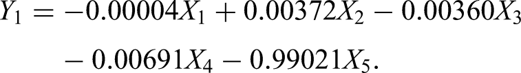
Table 1 presents the results of various regression analyses on both raw data and PCs.On the right-hand side of the table, the outcomes of employing different regression models in PCR and ICR are displayed. Given the presence of some noise in the initial data, we will also examine Ridge and Lasso regression models in addition to the OLS model. However, based on the values in this Table, using ridge and lasso regressions resolves this problem effectively. Additionally, the results of ICR are better than those of PCR and Multiple Linear Regression (MLR). The weaker results of PCR compared to MLR may be due to the removal of all less important principal components.

The main objective in the ICA process is to optimize this contrast function. This means applying optimization techniques to adjust the parameter values in such a way that the contrast function reaches its maximum or minimum, indicating the desired level of independence between the components has been achieved. The general equation for ICA is: $\mathit{X}\mathbf{=}\mathit{A}\mathit{S}$ , where $\mathit{X}$ is the matrix of mixed signals (variables) and $\mathit{A}$ is the mixing matrix, and $\mathit{S}$ is the matrix of the source signals. Each element of the mixing matrix is a real number. In fact, our goal at ICA is to find the mixing matrix $\mathit{A}$ and the source signal $\mathit{S}$ using by the matrix of the $\mathit{X}$ signal combinations. $\mathit{S}$ can be obtained by the relation: $\mathit{S}\mathbf{=}{\mathit{A}}^{\mathbf{-}\mathbf{1}}X$ . Mixing matrices and matrix signal sources are unknown, and this complicates our work. Hence the variables are also called hidden variables. Another ICA hypothesis is that the source signals are independent of each other and have an non-Gaussian distribution. The first step in ICA is to whitening $\mathit{X}$ . For this purpose, we use a new data matrix $\mathit{Z}\mathbf{=}\mathit{V}\mathit{X}$ , whose elements are uncorrelated and have a single variance. In other words: $\mathit{E}\mathbf{(}\mathit{Z}{\mathit{Z}}^{\mathit{T}}\mathbf{)}\mathbf{=}\mathit{I}$ .

Table 1.

$R^2$ and MRE for multiplie linear regression (MLR), PCR and ICR.

	MLR		PCR		ICR
	$R^2$	MRE	$R^2$	MRE	$R^2$	MRE
OLS	0.6910	0.2660	0.2535	0.3243	0.8871	0.2136
Ridge	0.8869	0.2071	0.6530	0.3013	0.8791	0.1980
Lasso	0.8871	0.2091	0.6521	0.3053	0.88709	0.2092

The matrix $\mathit{V}$ can be obtained by decomposing individual values such that: $\mathit{V}={\mathbf{\Lambda }}^{\mathbf{-}\mathbf{1}}{\mathit{P}}^{\mathit{T}}.$ Also, the $\mathit{P}$ columns are the special vectors of the covariance matrix $\mathit{Z}{\mathit{Z}}^{\mathit{T}}$ and the diagonal sentences $\mathbf{\Lambda }$ are equal to the eigenvalues. The second step is to define a separation matrix $(\mathit{W})$ that converts the $\mathit{Z}$ matrix to an $\mathit{S}$ matrix with non-Gaussian components and ICs: $\mathit{S}\mathbf{=}{\mathit{W}}^{\mathit{T}}\mathit{Z}.$

There are several ways to achieve this approximation: non-Gaussian maximization of ${\mathit{W}}^{\mathit{T}}\mathit{Z}$ gives us ICs. In other words, minimizing the mutual information between the columns of ${\mathit{W}}^{\mathit{T}}\mathit{Z}$ , minimizes the interdependence between them. The assumption of being non-Gaussian can be tested in several ways, Kurtosis and negative entropy are the most common of these methods, the first of which is sensitive to outlier data and the second is based on the entropy information quantity theory. Also, with histogram plots, the normality of the data can be discussed.

For ICA, in many studies, the details of the data whitening method are not explained. In the following, we will examine the data whitening process step by step with an example.

Example 2.2. This example contains failure data collected of the silver–zinc battery during its life cycle, Johnson (2007). ⁹ We assume the following predictors and outcome variables

$X_1$ : charge rate (amps), $X_2$ : dischrge rate, $X_3$ : depth of discharge, $X_5$ : temperature, $X_5$ : end of charge voltage, $Y$ : cycles to failure

To continue, we implement ICA on this data.

The vector of eigenvalues $(\mathit{\lambda })$ and the matrix of eigenvectors $(\mathit{V})$ are:

$$\mathit{\lambda }=(11009.593,236.919,51.939,1.95,0.192,0.00009),$$

$$\mathit{V}=\left[\begin{array}{cccccc}-0.00071& 0.01231& -0.00431& 0.00901& 0.99921& 0.00093\\ -0.00044& -0.01730& 0.00722& -0.99931& 0.00904& 0.00041\\ -0.02401& -0.98920& 0.14611& 0.01812& 0.01312& 0.00005\\ 0.06310& -0.14833& -0.98721& -0.00401& -0.00322& -0.00031\\ 0.000005& -0.000009& 0.00032& -0.00041& 0.00093& -0.99922\\ 0.99801& -0.01432& 0.06611& 0.00032& 0.00101& 0.00002\end{array}\right]$$

$$\begin{array}{rl}& \mathbf{\Sigma }=E(\mathit{D}{\mathit{D}}^{\mathit{T}})=diag[11009.59,236.92,51.94,1.95,\\ & 0.0019,0.00009],\end{array}$$

that, $\mathit{D}\mathbf{=}\mathit{X}\mathbf{-}\mathit{\mu }$ .

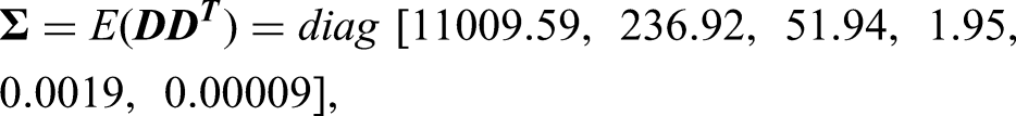
The data on both sides of the main diagonal are almost zero, so we considered their values are equal to zero. This means that the covariance between two mixture signals is zero. For rescale of the signals with a unit variance, we use equation: 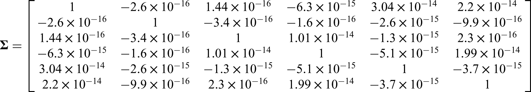$\mathit{Z}={\mathit{\lambda }}^{-\frac{1}{2}}\mathit{U}={\mathit{\lambda }}^{-\frac{1}{2}}\mathit{V}\mathit{D}$ , then The covariance matrix for the whitened data is:

$$\mathbf{\Sigma }=\left[\begin{array}{cccccc}1& -2.6\times {10}^{-16}& 1.44\times {10}^{-16}& -6.3\times {10}^{-15}& 3.04\times {10}^{-14}& 2.2\times {10}^{-14}\\ -2.6\times {10}^{-16}& 1& -3.4\times {10}^{-16}& -1.6\times {10}^{-16}& -2.6\times {10}^{-15}& -9.9\times {10}^{-16}\\ 1.44\times {10}^{-16}& -3.4\times {10}^{-16}& 1& 1.01\times {10}^{-14}& -1.3\times {10}^{-15}& 2.3\times {10}^{-16}\\ -6.3\times {10}^{-15}& -1.6\times {10}^{-16}& 1.01\times {10}^{-14}& 1& -5.1\times {10}^{-15}& 1.99\times {10}^{-14}\\ 3.04\times {10}^{-14}& -2.6\times {10}^{-15}& -1.3\times {10}^{-15}& -5.1\times {10}^{-15}& 1& -3.7\times {10}^{-15}\\ 2.2\times {10}^{-14}& -9.9\times {10}^{-16}& 2.3\times {10}^{-16}& 1.99\times {10}^{-14}& -3.7\times {10}^{-15}& 1\end{array}\right]$$

This means that the whitened data are uncorrelated and have unit variance.To achieve better results, we perform ICA on the whitened data.

Our approach

There are different algorithms available for performing PCA and ICA. For example, PCA can be done using classical algorithms or methods like Kernel PCA, Sparse PCA, Incremental PCA, and more. For ICA, algorithms such as FastICA, JADE, Infomax, ProDenICA (projection pursuit), RLICA (rank-based loss ICA), and others can be used. In many studies, the specific details and challenges of using PCA and ICA are often overlooked. If we have a set of real-world data, the question arises: without considering a specific goal and based solely on the properties and characteristics of the data, is it more appropriate to apply ICA or PCA?

In PCA, the main goal is to reduce the data dimensions while keeping as much variance as possible in the principal components. This is done by calculating the eigenvalues and eigenvectors of the covariance matrix, with the eigenvectors corresponding to the largest eigenvalues chosen as the principal components.

In ICA, our goal is to find combinations of the observed data that are statistically independent from each other. To achieve this, we use a function called the contrast function. The contrast function is a measure used to evaluate the level of statistical independence between the extracted components. In other words, this function helps us identify the components that are most independent from one another.

Diagonastic

If we have a dataset, should we use PCA or ICA for it? The answer to this question depends on our goal. However, sometimes we want to evaluate which method is more suitable for our data based solely on the initial structure of the data without any specific goal. Additionally, in some cases, the data structure indicates that ICA is more appropriate, but PCR performs better than ICR, and vice versa. Sometimes ICR performs better than PCR even though the initial data structure is more suited to PCA. What factors cause this issue?

As noted by Hyvärinen et al., ¹⁰ ICA is not efficient for Gaussian data. In our algorithm, the nature of the data is first assessed to determine whether its structure is more compatible with PCA or ICA. Subsequently, for each case, steps such as noise removal, outlier elimination, and selection of an appropriate regression model are performed to mitigate the inherent limitations of each method. Therefore, even in situations where the data are theoretically more suitable for ICA or PCA, our proposed algorithm can create conditions under which the corresponding regression (ICR or PCR) achieves better performance. This is precisely where our work introduces novelty compared to previous studies: rather than accepting the intrinsic limitations of ICA or PCA, we provide a framework that, through data preparation, alleviates these limitations to some extent and improves regression outcomes.

In this study, we have examined this issue in detail by drawing several flowcharts. The general flowcharts are as follows and a detailed diagram are depicted in appendix.

Numerical study

In this section, we test our approximation using simulations and real-world data analysis.

Simulation

In this simulation study, we first generate data from multivariate Normal distribution.

We assume that, 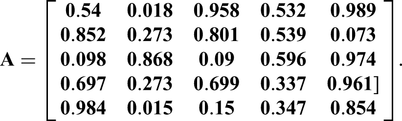$\mathbf{X}\sim {\mathbf{N}}_{\mathbf{5}}\mathbf{(}\mu \mathbf{,}\mathbf{\Sigma }\mathbf{)}$ , where $\mu$ = $(0.046,0.039,0.106,0.607,0.219)$ , $\mathbf{\Sigma }\mathbf{=}\mathbf{A}{\mathbf{A}}^{\mathbf{T}}\mathbf{,}$ where

$$\mathbf{A}\mathbf{=}\left[\begin{array}{ccccc}0.54& 0.018& 0.958& 0.532& 0.989\\ 0.852& 0.273& 0.801& 0.539& 0.073\\ 0.098& 0.868& 0.09& 0.596& 0.974\\ 0.697& 0.273& 0.699& 0.337& 0.961]\\ 0.984& 0.015& 0.15& 0.347& 0.854\end{array}\right]\mathbf{.}$$

The mean vector was empirically determined through repeated simulations and trial $-$ and $-$ error adjustments, aiming to produce a multivariate normal distribution with a structure suitable for PCA, while also creating conditions under which ICA performs better than PCA in regression tasks. Specifically, small asymmetric shifts were introduced to the mean of each dimension to preserve the linear correlation structure essential for PCA, while increasing the statistical independence among components, which is critical for ICA.

The choice of simulation parameters was guided by the dual objective of maintaining sufficient linear structure for PCA and creating conditions in which ICA could reveal hidden dependencies more effectively. Specifically, the mean vector $\mathit{\mu }$ , was determined empirically through repeated simulations and trial $-$ and $-$ error adjustments, ensuring the presence of linear correlations among variables while increasing relative independence across components. The matrix $\mathbf{A}$ , was selected so that the covariance $\mathbf{\Sigma }=\mathbf{A}{\mathbf{A}}^T$ , was meaningful and non-singular. Furthermore, the vector $\mathit{C}$ , was randomly generated to simulate regression coefficients. To verify robustness, alternative values for $\mathit{\mu }$ and $\mathbf{A}$ , were also tested, yielding qualitatively similar results. Hence, the outcomes are not tied to a specific parameter configuration and can be considered reliable.

Also the response variable is: $\mathbf{Y}\mathbf{=}\mathbf{C}\mathbf{X}\mathbf{+}\mathit{\epsilon }$ , where $\mathbf{C}$ is a vector contains 5 random numbers, and $\mathit{\epsilon }\sim \mathbf{N}\mathbf{(}\mathbf{0}\mathbf{,}\mathbf{1}\mathbf{)}$ . Then, we perform ICA and PCA on the simulated data, followed by regression on the ICs obtained from ICA and PCA. Next, for varying numbers of samples and repetitions, we compare the regression results of the main components with those of the ICs.

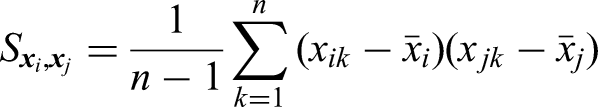
To compare ICR and PCR, we use two criteria: MSE (mean square error) and MRE (mean relative error), which are defined as

$$MSE=\frac{1}{n}\sum _{i=1}^n{(y_i-{\hat{y}}_i)}^2,MRE=\frac{1}{n}\sum _{i=1}^n\frac{|y_i-{\hat{y}}_i|}{y_i}\times 100$$

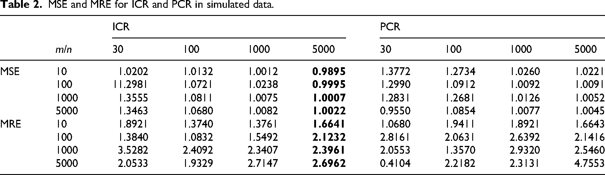
The simulation results in Table 2 show that the values of all three error criteria are lower in ICR than in PCR in most cases. According to the values of all three indicators for each iteration, when the sample size is high enough, the regression of ICs is more accurate than the regression of principal components. The simulated data structure is more suited to PCA than ICA, so PCR results are usually expected to be better than ICR. However, as seen in Table 2, ICR performs better than PCR with larger sample sizes. To resolve this, we followed steps from Algorithm 1, detailed further in Algorithm 2.

Table 2.

MSE and MRE for ICR and PCR in simulated data.

		ICR				PCR
	$m$ / $n$	30	100	1000	5000	30	100	1000	5000
MSE	10	1.0202	1.0132	1.0012	0.9895	1.3772	1.2734	1.0260	1.0221
	100	11.2981	1.0721	1.0238	0.9995	1.2990	1.0912	1.0092	1.0091
	1000	1.3555	1.0811	1.0075	1.0007	1.2831	1.2681	1.0126	1.0052
	5000	1.3463	1.0680	1.0082	1.0022	0.9550	1.0854	1.0077	1.0045
MRE	10	1.8921	1.3740	1.3761	1.6641	1.0680	1.9411	1.8921	1.6643
	100	1.3840	1.0832	1.5492	2.1232	2.8161	2.0631	2.6392	2.1416
	1000	3.5282	2.4092	2.3407	2.3961	2.0553	1.3570	2.9320	2.5460
	5000	2.0533	1.9329	2.7147	2.6962	0.4104	2.2182	2.3131	4.7553

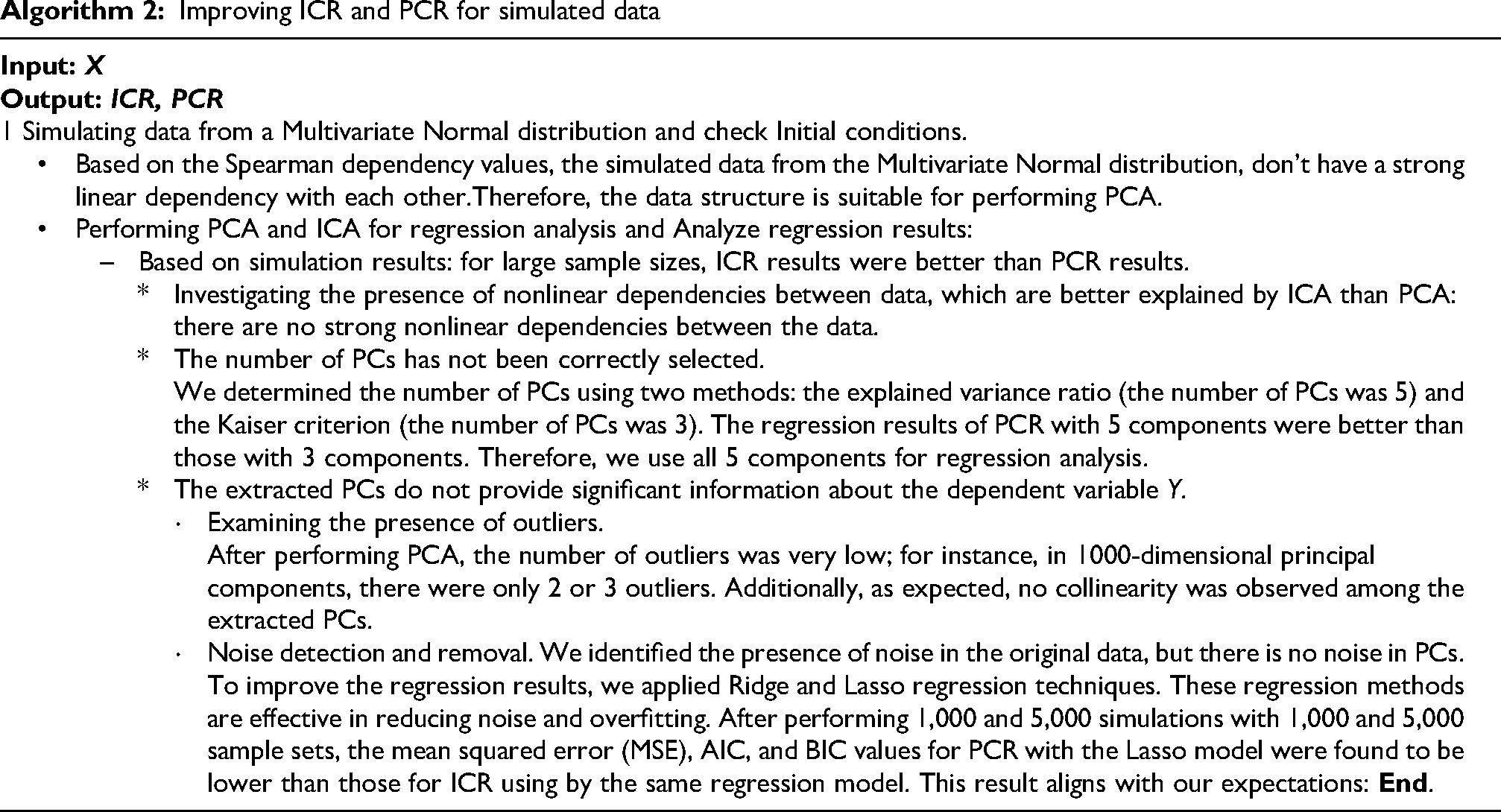
Given that after running Algorithm 2, the values obtained for MSE, AIC, and BIC in Table 3 for the Lasso regression model in PCA are lower than those in ICA, we conclude that to improve PCR regression, it is better to use Lasso regression instead of simple linear regression to achieve the desired results.

Table 3.

MSE, AIC and BIC for simulation data.

	ICR $(m=1000,n=1000)$			PCR $(m=1000,n=1000)$
	MSE	AIC	BIC	MSE	AIC	BIC
OLS	1.013	13.297	32.455	1.691	93.029	104.297
Ridge	1.457	77.264	96.422	1.670	90.577	101.845
Lasso	2.458	167.491	186.652	1.670	90.579	101.847

	ICR $(m=5000,n=5000)$			PCR $(m=5000,n=5000)$
	MSE	AIC	BIC	MSE	AIC	BIC
OLS	1.011	12.039	40.854	1.650	417.148	433.919
Ridge	1.441	332.676	361.491	1.650	417.148	433.919
Lasso	2.424	782.206	811.021	1.672	430.522	447.294

The results in Tables 3 indicate that by following Algorithm 2, we can improve the PCR regression model.

Real data

In the following, we perform PCA and ICA on real data and compare these two methods. We want to discuss which of the two types of component analysis, ICA or PCA, is better suited for our data based solely on the initial structure of the data without considering the goals of PCA and ICA.

Concrete data

These data correspond to 1030 observations of the complete compressive strength of a mixture of different raw materials. This dataset includes eight predictor variables, which are as follows:

1- Cement (kg), 2- Blast furnace slag, 3- Fly Ash, 4- Water, 5- Super plasticizer,

6- Coarse Aggregate, 7- Fine Aggregate, 8- Age (According to the day).

The dependent variable is: the compressive strength of concrete.

At first, we performed ICA using the Fastica method on the data and illustrated the linear trend and histograms of each original variable (mixture) in Figure 1 and the linear trend and histograms of the ICs extracted from ICA in Figure 2. According to the histograms, the distribution of the ICs was non-normal, while the original data followed a normal distribution. This indicates that the initial conditions for ICA are met.

Figure 1.

Eight mixtures in Real data, and their histograms.

Figure 2.

Eight sources in real data, and their histograms.

Given that our raw data are non-normal and exhibit weak nonlinear relationships, performing ICA is more appropriate than PCA. After ICA on the data, the results of regression on the ICs were found to be unsatisfactory, with an R² value of $0.414$ . But in PCR, the R² value was found to be 0.605. So, we tried to analyze ICA more carefully.

To further investigate this difference, scatter plots of each IC against concrete compressive strength ( $Y$ ), were generated, and third $-$ degree polynomial fits were applied to reveal potential nonlinear patterns (Figure 3). The shapes of some ICs (e.g., ${\mathrm{IC}}_2$ and ${\mathrm{IC}}_7$ ) indicate that their relationships with the response variable are nonlinear, whereas others (e.g., ${\mathrm{IC}}_1$ and ${\mathrm{IC}}_5$ ) display curvature suggestive of higher-order dependencies. These plots demonstrate that linear regression cannot fully capture the dependence between ICs and compressive strength. Applying third-degree polynomial regression substantially improves predictive performance ( $R^2$ increased) and highlights the necessity of nonlinear modeling when using ICs as predictors.

Figure 3.

Nonlinear patterns between independent components and concrete compressive strength.

To further investigate the difference between the $R^2$ values in ICR and PCR, we quantified the nonlinear characteristics of the data. Specifically, we computed higher $-$ order moments (skewness and kurtosis), Pearson and Spearman correlations (to capture linear and monotonic nonlinear dependencies), as well as mutual information (Table 4). This table shows descriptive statistics, dependency measures, predictive power ( $R_{\mathrm{single}}^2$ ), and absolute contribution (AbsContribution) for the original variables, PCA components, and ICA components. Absolute contribution is only meaningful for combined components (PCs or ICs) and is not defined for raw variables. The results show that in the raw data, some variables (such as Age) exhibit strong skewness and kurtosis, indicating significant deviations from normality. In addition, for certain variables (e.g., Age and Water), the Spearman correlation is noticeably higher than the Pearson correlation, which confirms the presence of nonlinear relationships with the compressive strength of concrete. The transformed components also revealed comparable patterns, but with a key distinction: in most cases, the ICA components exhibited greater skewness and kurtosis, indicating their sensitivity to higher-order moments, whereas PCA primarily accounted for linear variance. These results provide a clear explanation for the performance difference observed between ICR and PCR: ICA reveals nonlinearities and non-normality in the data, making its extracted components less compatible with simple linear regression, while PCR, being based on linear variance, performed better in this setting. To test this hypothesis, we further applied third-degree polynomial regression on the ICs, which increased the $R$ value to 0.8391. This substantial improvement demonstrates that nonlinear relationships are the main reason behind the weak performance of linear ICR and that selecting a regression model aligned with the nonlinear structure of the data can dramatically enhance component analysis. All the steps of this process are summarized in Algorithm 3, see also Figure 6(diagram B) of appendix for more detail.

We will now provide some explanations regarding the algorithm.

Table 4.

Comparison of descriptive and dependency indices for raw variables, PCA, and ICA.

Type	Variable	Skewness	Kurtosis	PearsonCorr	SpearmanCorr	MI	$R_{single}^2$	AbsContribution
Original	Cement	0.509	$-$ 0.524	0.498	0.478	0.309	0.248	–
Original	Blast Furnace Slag	0.800	$-$ 0.512	0.135	0.164	0.181	0.018	–
Original	Fly Ash	0.537	$-$ 1.328	$-$ 0.106	$-$ 0.078	0.120	0.011	–
Original	Water	0.075	0.116	$-$ 0.290	$-$ 0.308	0.361	0.084	–
Original	Superplasticize	0.906	1.399	0.366	0.348	0.213	0.134	–
Original	Coarse Aggregate	$-$ 0.040	$-$ 0.602	$-$ 0.165	$-$ 0.184	0.257	0.027	–
Original	Fine Aggregate	$-$ 0.253	$-$ 0.108	$-$ 0.167	$-$ 0.180	0.216	0.028	–
Original	Age	3.264	12.104	0.329	0.596	0.358	0.108	–
PCA	PC1	0.502	$-$ 0.331	0.447	0.436	0.302	0.200	0.080
PCA	PC2	0.526	$-$ 0.598	0.237	0.255	0.295	0.056	0.048
PCA	PC3	0.324	$-$ 0.070	0.102	0.093	0.266	0.010	0.024
PCA	PC4	0.551	$-$ 0.275	0.115	0.181	0.245	0.013	0.036
PCA	PC5	2.813	10.179	0.164	0.179	0.350	0.027	0.053
PCA	PC6	0.096	$-$ 0.747	$-$ 0.551	$-$ 0.544	0.426	0.304	0.325
PCA	PC7	0.024	2.175	$-$ 0.057	$-$ 0.072	0.225	0.003	0.135
PCA	PC8	0.135	2.509	$-$ 0.050	$-$ 0.057	0.196	0.002	0.299
ICA	IC1	$-$ 0.094	2.142	$-$ 0.144	$-$ 0.129	0.244	0.021	0.069
ICA	IC2	1.620	4.429	0.449	0.395	0.322	0.202	0.217
ICA	IC3	$-$ 3.276	12.170	$-$ 0.293	$-$ 0.476	0.485	0.086	0.142
ICA	IC4	$-$ 0.541	2.057	$-$ 0.365	$-$ 0.332	0.348	0.133	0.176
ICA	IC5	$-$ 0.129	0.609	$-$ 0.172	$-$ 0.181	0.192	0.030	0.083
ICA	IC6	$-$ 0.079	$-$ 1.317	$-$ 0.193	$-$ 0.231	0.354	0.037	0.093
ICA	IC7	0.198	$-$ 0.961	0.272	0.280	0.246	0.074	0.132
ICA	IC8	$-$ 0.677	5.234	$-$ 0.182	$-$ 0.165	0.214	0.033	0.088

There were a lot of outliers in the extracted ICs (211 in total), and it didn’t make sense to just get rid of them because we’d lose some important information about how the independent variables relate to the dependent one. So, we tried to reduce the effect of the outliers by using a customized FastICA method and swapping the usual normal distribution with a Truncated normal distribution. This helped reduce the outliers, but it didn’t really change the $R^2$ value much.

To lessen the impact of outliers in the extracted ICs, we can swap the normal distribution with the Laplace or t distribution. These distributions have heavier tails than the normal one, which means they handle outliers better.

Therefore, using the Akaike criterion, we compared the whitened data distribution with normal, exponential, gamma, beta, $t$ , and Laplace distributions and concluded that our data, after whitening, follows a t-distribution with parameters: 8.87, -0.036, and 0.875. So, we performed ICA using a customized fastICA method with a t-distribution having parameters 8.87, -0.036, and 0.875. This reduced the number of outliers to 61 data points; however, the regression results weakened, and the $R^2$ value decreased to 0.168. Therefore, besides the presence of outliers, other issues might have contributed to the regression results weakening. We investigated some potential problems:

Presence of noise in the data extracted by ICA: our data contained 28 noise points, which we removed before conducting the regression. However, the regression results worsened. With the decrease in the $R^2$ , we concluded that by removing the noise, some information about the dependent variable $Y$ present in the independent variables was lost.

The independent variables extracted by ICA do not contain much information about the dependent variable $Y$ (concrete compressive strength): this means that the data extracted by ICA may not have captured important features related to the dependent variable. By calculating Pearson correlation coefficients between the independent variables and the dependent variable $Y$ , it was observed that the first, second, and eighth independent variables have a very weak relationship with $Y$ , and this relationship is moderate for other independent variables. Additionally, the Spearman correlation coefficients for some of these variables were higher than the Pearson correlation coefficients, indicating that there might be some nonlinear relationships between certain independent variables and the dependent variable $Y$ .

Nonlinear Relationship: The relationship between the independent variables obtained from ICA and the dependent variable $Y$ may be nonlinear. Considering Figure (4), some heteroscedasticity in the variance of predicted values is observed. Additionally, as the residuals depict a nonlinear trend (resembling a funnel shape), it can be inferred that the relationship between the independent and dependent variables may be nonlinear.

To recognize nonlinear relationships between independent variables and $Y$ we generate polynomial features for the independent variables, fit an ANOVA model with polynomial terms, and prints a summary of the ANOVA model .

In this model, the $R^2$ value is 0.647, indicating that approximately 64.7 percent of the variance in concrete compressive strength is explained by the independent variables in the model. Since the value of $R^2$ in the ANOVA table has increased compared to this value in ICR (linear regression for ICs), it can be concluded that there are some nonlinear relationships between ICs and the variable Y.

Lack of Fit and Overfitting: This model may be too simplistic to capture the complexity of the relationship between the data obtained from ICA and the concrete compressive strength. Therefore, to improve the $R^2$ and resolve the mentioned issues, we have used the following methods:

i- Feature engineering: Meaning, during the extraction of ICs, extracting additional informative features from the data that have better correlation with the compressive strength of concrete.

By employing this method, $R^2$ in the regression model became equal to one, which is not a reliable result.

ii-Ridge regression and Lasso regression: Because there is some correlation among several of the extracted ICs, and non-random patterns are observed in the scatter plots of residuals against predicted values, our regression model exhibits some degree of both linearity and overfitting. To resolve this issue and also the presence of noise in the data, we employ Ridge regression and Lasso regression for conducting ICR.The values of $R^2$ in Ridge and Lasso regressions were obtained as 0.4148 and 0.4139, respectively, which does not differ significantly from the $R^2$ value in simple linear regression. By employing polynomial regression in ICR, the $R^2$ value will be 0.8391. Therefore, selecting an appropriate regression model according to the data structure will play a crucial role in component analysis.

Figure 4.

Plot of residuals versus predicted values for ICA data.

Heart data

This dataset, collected from the Kaggle website, contains medical records of 299 patients with heart failure. The records were gathered during their follow-up period, and each patient’s file includes 12 clinical features and a response variable, which are:

$X_1:$ age of the patient,

$X_2:$ anemia(decrease of red blood cells or hemoglobin),

$X_3:$ creatinine-phosphokinase (level of the CPK enzyme in the blood),

$X_4:$ diabetes (if the patient has diabetes),

$X_5:$ ejection fraction (percentage of blood leaving the heart at each contraction),

$X_6:$ high blood pressure (if the patient has hypertension),

$X_7:$ platelets (platelets in the blood),

$X_8:$ serum creatinine (level of serum creatinine in the blood),

$X_9$ : serum sodium (serum sodium),

$X_{10}$ sex (woman or man),

$X_{11}:$ smoking (if the patient smokes or not),

$X_{12}:$ time (follow-up period),

$Y:$ death event (if the patient died during the follow-up period).

To analyze the data structure, we first conducted the Kolmogorov–Smirnov test and examined the $Q-Q$ plot, which indicated that the data dont have normal distribution.

Additionally, by calculating Pearson and Spearman correlation coefficients for each variable, we identified nonlinear dependencies among the variables. Therefore, the data appeared suitable for applying ICA. The heart failure dataset also exhibited strong non-Gaussian structures: variables such as creatinine phosphokinase and serum creatinine showed extreme skewness and kurtosis (above 20), while others such as time and serum creatinine revealed substantial nonlinear associations (as captured by Spearman correlation and mutual information). These nonlinearities limit PCA, which relies on linear correlations and variance, whereas ICA, by leveraging higher-order statistics, can extract components with stronger predictive power (as reflected by larger AbsContribution and $R_{\mathrm{single}}^2$ ). This property explains the observed performance gap between ICR and PCR under nonlinear data conditions. We began by implementing ICA using the FastICA algorithm on the dataset. Subsequently, we performed regression analysis between the extracted ICs and the response variable. Next, we applied PCA on the original data, selected the PCs that explained the most variance based on their eigenvalues, and performed regression between these components and the response variable.

The $R^2$ values for ICR and PCR were 0.303 and 0.444, respectively. Against our expectations, the PCR results were better than the ICR results. Guided by our proposed algorithm, we explored alternative approaches to improve the results of ICA regression.

Based on the software output, since the FastICA algorithm did not fully converge, we applied the Box–Cox transformation to the data, normalized them, and removed outliers. Then, we re-applied the FastICA method to extract ICs and performed ICR. With the convergence of the FastICA algorithm after these steps, the ICR results showed slight improvement, and the R-score reached 0.454.

To further improve the regression performance of ICR, we removed noise from the raw data and repeated the ICA and ICR processes. This led to an increase in the R-score to 0.470.

After performing cross-validation, slight overfitting was observed in the extracted ICs. Therefore, instead of using standard linear regression in ICR, we used Ridge and Lasso regression. The R-scores for Ridge and Lasso regression were 0.4703 and 0.221, respectively, indicating no significant improvement in the regression results.

In the next step, to explore possible nonlinear relationships and more complex dependencies in ICR regression, we used polynomial (second-degree) and spline regression. The R-scores for polynomial and spline regression were 0.622 and 0.643, respectively. These results show that using more suitable regression models can significantly improve the performance of ICR. In Table 5, we show the ICR regression results for different regression model selections: According to the data in Table 5, after removing noise and outliers and normalizing the data, the use of polynomial and spline regression significantly improved the performance of the ICR regression. Based on the $R^2$ values and the mean squared error, spline regression is identified as the best-performing method.

All the steps of this process are summarized in Algorithm 4.

Table 5.

MSE & $R^2$ after using different regression models in ICR.

	OLS	Ridge	Lasso	Polynomial	Spline
$R^2$	0.470	0.4703	0.221	0.622	0.643
MSE	0.116	0.115	0.169	0.082	0.078

Results

In this article, we aimed to explore the results of ICR and PCR using practical examples on both real and simulated data, with detailed explanations. Additionally, we demonstrated how to preprocess data for performing ICA using a practical example on real data. Sometimes, we may want to know which method, ICA or PCA, works better based solely on the data’s structure, without a specific goal in mind. Suppose ICA performs better than PCA and all necessary conditions for ICA are met. However, when comparing the regression results of ICR with PCR, we might find that PCR performs better than ICR. In this article, we provided several practical examples where we examined these contradictions in detail, step by step. Based on the results obtained, the initial structure of the data plays a significant role in both ICA and PCA. After whitening the data in ICA, it’s advisable to first analyze the resulting whitened data structure ( ${\mathit{z}}_{\mathit{i}}$ ) and consider using a customized FastICA method instead of the standard approach, which aligns with the data’s structure rather than assuming a Normal distribution. Also, factors like outliers and noise can weaken the regression results of ICR. In such cases, improving results can be done by removing noise, replacing or deleting outliers (if it does not lead to significant data loss). Otherwise, it’s better to use more suitable regression models like ridge regression and lasso regression. If there are nonlinear relationships among our variables, applying polynomial regression can improve the results from ICR. Furthermore, by simulating data from a Multivariate Normal distribution with sample sizes of 30, 100, 1000, and 5000, and repetitions of 10, 100, 1000, and 5000, we show that when raw data follow a Multivariate Normal distribution and meet the necessary conditions for ICA, ICR performs more accurately than PCR, especially with sufficiently large sample sizes.

In the following part of this study, advanced optimization algorithms can be used for feature selection and improving model performance. Additionally, dimensionality reduction techniques (such as PCA) can be combined with various regression methods to increase prediction accuracy.

This study demonstrates that the targeted application of ICA in regression modeling can lead to significant improvements under non-Gaussian data conditions. However, the choice between ICA and PCA should be based on the nature of the data distribution, structural complexity, and modeling objectives.

Discussion and conclusion

In this study, we first examined the preprocessing steps involved in ICA, with a particular focus on data whitening. We then compared the performance of ICR and PCR using both real-world and simulated datasets, supported by practical examples. The results underscored the critical role of the underlying data structure in shaping the effectiveness of both ICA and PCA. While ICA may outperform PCA under ideal conditions (and vice versa), the practical outcomes are often influenced by factors such as noise, outliers, and non-ideal data distributions.

Preprocessing, especially the whitening stage in ICA, was emphasized as a key step. Careful analysis of the whitened data is recommended to select the most suitable method (potentially a customized variant) based on the specific properties of the dataset, rather than assuming normality. Additionally, mitigating noise and handling outliers effectively were found to significantly enhance the performance of both ICA and PCA, as well as their respective regression models.

The choice of regression technique also plays a vital role in the performance of ICR and PCR. In scenarios where overfitting is a concern, regularization methods such as Ridge and Lasso regression can be effective. For datasets exhibiting nonlinear relationships, models like polynomial regression may yield superior results.

Future research should aim to develop more robust ICA and PCA algorithms that are less sensitive to outliers, along with adaptive systems that can recommend the most appropriate regression model based on data structure. Furthermore, designing algorithms based on statistical tests that automatically determine whether ICA or PCA is more suitable for a given dataset could provide a valuable decision-making tool for method selection.

Although the case studies used in this research (such as concrete strength and heart disease data) demonstrate the effectiveness of the algorithms, further analysis on a broader variety of datasets is needed to generalize the findings to other data structures.