
Abstract
Using topological summary tools such as persistence landscapes have greatly enhanced the practical usage of topological data analysis to analyze large-scale, noisy, and complex datasets. A central element of persistence landscape usage involves computing the top-
Keywords
Introduction
Topological data analysis (TDA) is the application of topological functions and methods to datasets in order to gain greater insight into the properties of a dataset. It is based on the work done in algebraic topology and promises to provide more robust methods than those based on geometric metrics due to its focus on properties which persist under continuous deformation. It has shown to be an effective way at gaining insight into datasets in a new way.1–3 Due to providing some initial promising results in fields which traditionally struggle with noisy, high dimensional and incomplete datasets, there is an increasing amount of research efforts.
TDA has been shown in some cases to give data scientists a new way to understand and explore the underlying structure of their data by allowing them to compute the topology of the data. Since its initial discovery, different data structures and techniques with varying properties have been presented, enabling rising interest for their application in data science and machine learning. Although, it is still an open problem for how to best incorporate the information for machine learning.
The discovery of persistent homology allowed for the ideas from algebraic topology to be applied to the point clouds seen in data science and machine learning.4,5 Persistent homology can be represented in many different forms. Bubenik et al. 6 introduced a representation that holds desirable statistical properties: the persistence landscape (PL). Among these properties is being stable under perturbation which is useful in machine learning. Persistent homology allowed researchers to apply TDA techniques to datasets and use existing statistical machine learning algorithms. As topology captures the invariants of a dataset under continuous deformation, it has been seen that these properties have better generalizability in some problem domains than geometric properties.1,7
Machine learning pipelines using PL have performed competitively in some time series classification for networking datasets,
7
and time series prediction in financial markets.2,3 Unfortunately, the algorithms for computing PL are not well suited for larger datasets. The best algorithm for computing the top-
This article introduces novel algorithms to address this issue. It presents algorithms which have a lower time complexity than the previous state-of-the-art. The presented algorithms only compute a constant number of extraneous operations for each returned landscape segment, making the algorithm output sensitive. Some algorithms’ time complexity can be better expressed in terms of both their input and output size when their output size can vary greatly. The algorithms are output sensitive algorithms and are common in computational geometry. Thus, the algorithm sees the greatest relative speed up when the top-
This output-sensitive algorithm is made possible by taking advantage of a new relationship between persistence pairs and PLs. Due to this relationship, we have provided an algorithm that can determine with
This article’s novel algorithm for PL generation from a set of birth-death pairs is the new state-of-the-art in terms of asymptotic complexity when computing the top-
The work presented here provides the following novel contributions
Improving the computation of PL by only a single pass over the data with optimal time complexity (this is of crucial concern when the entire dataset cannot fit in memory) Filtering the persistence pairs to remove noise (not discussed by Bubenik et al.
8
) and of importance to PL’s use in noisy datasets, an area PL has been applied to and found success in. Quantifying the speedups that can be expected when limiting the number of landscapes returned (using synthetic and real-world datasets). Providing an implementation of the algorithms in Rust with Python bindings.
This article proceeds as follows: the “Related work” section discusses related work in TDA, the “Background” section provides a background of the elements of TDA, the “Algorithms” section presents the novel algorithm for PL generation and its runtime analysis, the “Persistence pairs filtering” section presents the persistence pairs filtering algorithm and its runtime analysis, the “Experiments” section contain experiments done comparing this algorithm against the previous best on synthetic and real world datasets, and the “Conclusion” section provides a conclusion and summary of the results.
Related work
TDA is concerned with calculating topological invariants of datasets. Topological invariants from algebraic topology are concerned with computing the properties of spaces that are unchanged under continuous deformation. The use of global structures contrasts with geometric properties that are concerned with local structures in the data. This enables TDA techniques to be resilient to high noise levels in the data. The most common invariant to track in TDA is persistent homology. The seminal work on persistent homology4,5,9 enabled the application of algebraic topology on point cloud data. Persistent homology gives a multiscale interpretation of the data, allowing its topology to be computed and tracked at varying levels of connectedness. Other topological structures have built on persistent homology to add other properties of interest. One of these extensions, the PL,
6
is stable under perturbation and lives in a Banach or Hilbert space, allowing it to be used in statistical machine learning models. Bubenik et al.
6
also introduced the idea of the
PLs have found applications in many domains including financial market prediction,2,3 improving deep learning,1,10 brain artery trees, 11 music recognition, 12 similarity of pore-geometry in nanoporous materials, 13 and functional networks. 14
There are other TDA methods that capture persistent homology, including persistence images, 15 which have seen success in time series forecasting,16,17 3D shape segmentation 18 and for studying point clouds. 19 Persistence images allow for the use of machine learning techniques from computer vision to be used by embedding topological properties in matrices.
Bubenik et al.,
8
who originally introduced PLs,
6
presented a method for generating PLs from a set of birth-death pairs. They accomplish this by performing a sort on the set of birth-death pairs, followed by a single scan of the ordered set of pairs for each landscape to be generated. This results in a time of
Although the exact algorithm from Bubenik et al.
8
has optimal worst-case time with respect to the input size of the problem, it does this at the detriment of the more likely case that there are less than
There are also two other areas where unnecessary work can be avoided. First, the original algorithm considers every birth-death pair during the PLs calculation. If only the top-
Additionally, the original, exact algorithm makes
Background
TDA is a group of techniques that take advantage of a dataset’s topology to gain further insight into the data. It has been used with datasets that are noisy, incomplete, and have high dimensionality. Additionally, algorithms for efficiently computing meaningful representations for point clouds have been introduced for statistical learning. A central topic of TDA and the technique used by PL is persistent homology. Persistent homology captures the geometry of a point cloud by quantifying the shape and lifetime of the various n-dimensional “holes” within the point cloud. For a comprehensive self-contained mathematical introduction to TDA see Postol. 20
Simplices and simplicial complex
The starting point in TDA is the analysis of simplicial complexes. Simplicial complexes are a geometric notion of an abstract simplicial complex. An abstract simplicial complex is a family of sets that are closed under subsets (i.e. all subsets are valid members of the family of sets). Informally, simplices generalize the notion of a line or triangle to n dimensions. More formally, an n-simplex is a polytype of n dimensions defined as the convex hull of its
Filtrations
Filtration is a way of building up a simplicial complex starting from the empty set. Additionally, filtrations are indexed and totally ordered:
One standard filtration used in TDA is the Vietoris-Rips filtration, commonly known as the Rips filtration. The Rips filtration uses a set’s geometric properties to derive topological properties. Given a collection of points, define a threshold
-Skeleton
The
Persistent homology and persistent cohomology
Persistent homology and cohomology are both used in TDA, and, in most cases, produce equivalent results when their results are represented in a persistence representation. 21 from a practitioner’s
They are used to transform an ordered set of simplicial complexes from a filtration into birth-death pairs. These birth-death pairs represent the first and last threshold from the filtration that a topological property was observed during the filtration. Persistent homology and cohomology can be computed in various dimensions, where the dimension determines the type of topological objects being tracked.
This is typically visualized in lower dimensions as follows: 0-d persistent homology represents connected components; 1-d persistent homology represents “holes,” and 2-d persistent homology represents “voids.” Although this does not easily generalize to higher dimensions, some readers may find the intuition helpful homology at large.
It should be noted that some features may not have a numerical death value (represented in our framework as a death of
Persistence representations
There are multiple ways to visualize the birth-death pairs. Barcodes are made by creating a number line for the threshold value. Then, for each birth-death pair, a line is created starting at the birth and ending at the death. Usually, these lines are drawn not to intersect each other to create a more pleasing visualization. Another persistence representation is the persistence diagram, where the birth-death pairs are plotted in 2-d.
Persistence landscapes
To compute the PL, we take the birth-death pairs, and for each pair, we create two line segments. The first line segment will start at (b, 0), where b is the birth of that pair, and end at

Suppose a birth-death pair has a greater “lifespan” (the difference between birth and death) than another. In that case, the pair with the longer lifespan in the PL will peak higher than the other. This quantifies a feature’s importance overall and at a specific threshold by observing the height. We have a PL once we create all of these line segments and plot them on the same graph. The

Persistence landscape.
A key element of PLs and a main motivator for their creation and adoption in machine learning is that they are stable under perturbation. This stability allows them to be more easily compared in noisy environments than other topological representations, such as persistence barcodes and persistence diagrams. The goal is that this allows for statistical machine learning algorithms to take advantage of PLs with minimal modification. It should be noted that determining the optimal way to use topological information in machine learning models is still an open problem. Additionally, a PL exists in a Banach or Hilbert space, which makes the formulation of some statistical properties easier.
Algorithms
Two novel algorithms are presented in this section that, when combined, result in a significant speedup in the time needed to compute the top-
It should be noted that the persistence pair filtering step does not need to be done, as it is only for computational efficiency. Additionally, the persistence pairs filtering step can be used with any other algorithm for generating PLs from birth-death pairs. This is because it both takes in and outputs a set of birth-death pairs in the same format.
Plane-sweep landscape generation
This section provides an output-sensitive algorithm for computing PLs by taking advantage of the geometric structure of the problem. Bubenik et al. 8 were the first to propose that this might be helpful.
First, it is helpful to understand the simplest manifestation of the problem and build up from there. Given a collection of every birth-death pair and every intersection between birth-death pairs (including which two pairs are involved in the intersection), it is trivial to determine the top-
Fortunately, through careful modifications to the brute force algorithm, it is possible only to perform a minimal amount of additional work for each birth-death pair that appears in the top-
Secondly, we define an algorithm that checks for intersections only with birth-death pairs currently a part of the top-
To add new birth-death pairs into the top-
This algorithm is inspired by the basic line segment intersection algorithm taught in computational geometry. 22 When observing the PL problem from an abstract level, the two problems are similar.
Intersection discovery order
When we add a line segment to our working set, it is simple to calculate all the intersections of this new segment with all the previous existing segments. This can be done quickly,
Base case: The first line we add is correct and belongs to the top landscape, as there are no other segments in the working group. It is therefore in a valid state.
Induction: Add the next line and the resulting intersections. Without loss of generality, consider a single of these new intersections. The intersection can only be added to one landscape and must be the next intersection for the landscape. If it were not, then that means there is a line segment that intersects the line segment formed by the current last point in the landscape and our new proposed point.
Case 1: If this segment has a positive slope, then we are saying we are missing a negative slope segment, Case 2: If this segment has a negative slope, then we are saying we are missing a positive slope segment,
Conclusion: After each line segment and intersection, we maintain the correctness of the working group. Once all line segments and intersections are added to the working group, the landscapes of the working group are the correct landscapes overall.
This shows that intersections are added when they are discovered and do not need to be sorted or tracked (other than appending them to the output list for each
Compute top-
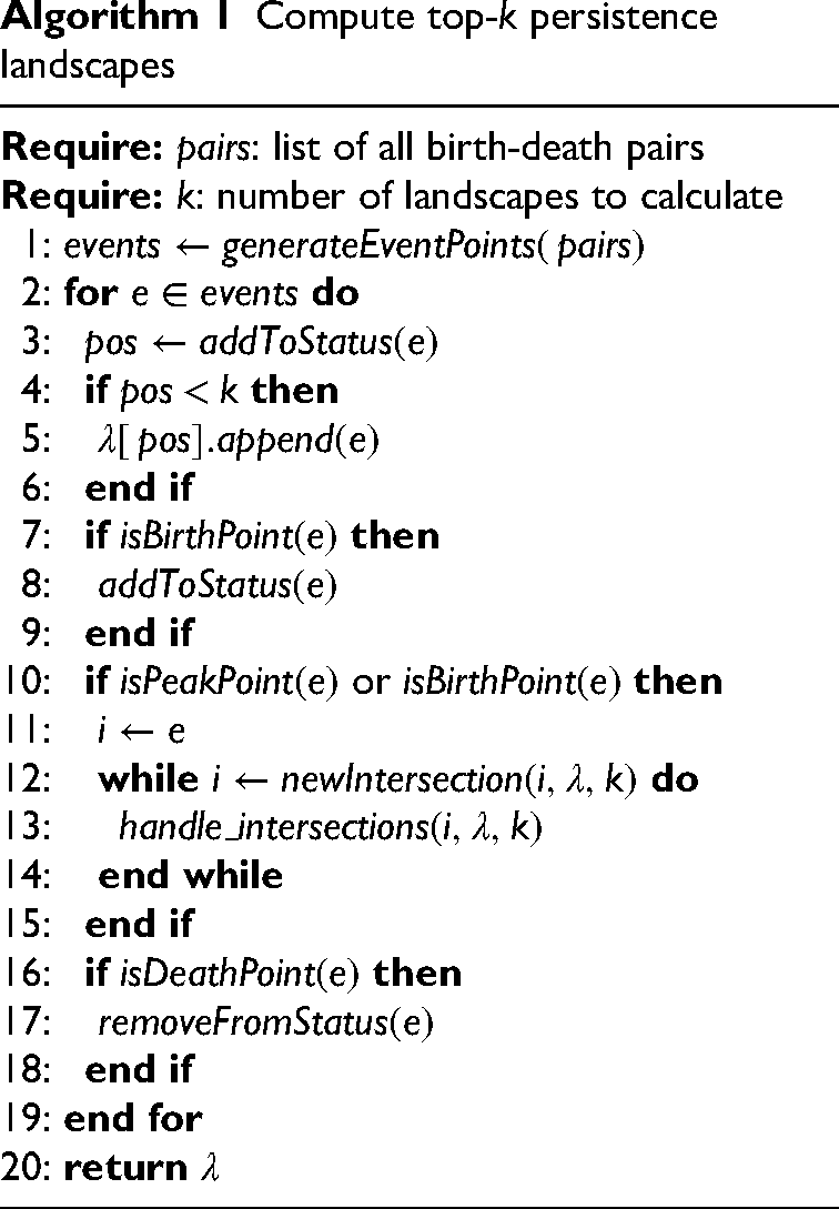
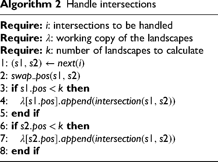
Handle intersections
Implementation details
Algorithm 1 contains the critical points of the algorithm but does leave out some bookkeeping. The rest of this section aims to fill in those gaps.
The algorithm is inspired by the plane-sweep line segment intersection. 22 Our algorithm differs from the original algorithm in the following key ways. We still have an ordering, but now our geometric objects consist of two line segments, defined by three points: birth, peak, and death. One line segment goes from birth to peak, and the other line segment goes from peak to death. Our status structure is the ordering of birth-death pairs, where having a higher y-coordinate at the sweep line’s current position denotes a higher position in the status structure. We should also note that our sweep line always starts on the far left of our collection of objects perpendicular to the x-axis. Our event points are the birth, peak, and death points that define each persistence pair in the PL. We check for intersection points the same way as in the line segment intersection algorithm: only checking for intersections between two pairs if they are neighbors in the status structure.
The algorithm does the following, given a set of birth-death pairs. First, it generates the initial event points in line 1. The initial event points correspond to the following for each birth-death pair: the birth, the peak, and the death of a given topological feature.
We need to take different actions at each event point. At a birth point, we must add the corresponding persistence pair to the status structure in line 3. From the definition of birth-death pairs, we can guarantee that when a persistence pair first appears; it must be lower than any other persistence pair in the status structure. As a result, we do not have to search the status structure to determine where it should be inserted to maintain the ordering. This fact allows us to get away with a simple status structure with constant insert and access times, such as a linked list. We must also check to see if this new persistence pair intersects with its neighbors in line 10, but because it is at the bottom of the status structure, it can only have one neighbor: the pair above it. We only check for this intersection if the neighbor above is after its peak. If it is still rising, it could switch positions with persistence pairs above it before intersecting with our new pair. If our new pair intersects with its neighbor, handle the intersection by swapping positions and logging to the output if needed, and then recursively check for any more intersections that may now exist. Finally, if our new pair has a position in the status structure in the top-
We check in with our bookkeeping for peak points to see if the peak point belongs to a persistence pair that is part of the top-
Lastly, we can guarantee that the corresponding persistence pair must be in the bottom position in the status structure for a death point. If this were not the case, then there would be at least one other point, the one below it, that would have to end earlier or intersect with our persistence pair before it could die itself. The reason is that all persistence pairs must end at the same y coordinate; they all have the same slope after their peak, and each persistence pair consists of only two line segments in the PL. As a result, we can delete the bottom persistence pair from the status structure, and be confident that it is the one the end point is referencing in line 16. Before we do this, we check to see if it is currently part of the top-
Runtime
The algorithm’s runtime is relatively complex to analyze, especially when combined with the results from the “Persistence pairs filtering” section and the “Intersection discovery order” subsection. First, for every event point, we only do constant work, not including handling intersections. This is because the three possible actions for an event are as follows: add to status (birth), check for intersection (birth, peak), add to a linked list (all), and remove from the status structure (death). For all of these actions, we maintain pointers between all the structures and, with proper bookkeeping, only incur an addition of
As the number of intersections per given structure of the same input size can vary greatly, it is crucial to consider the output-sensitive runtime of the algorithm. An algorithm that always performs as if every birth-death pair intersects would be leaving significant performance on the table if the number of intersections,
Additionally, due to being able to perform in-place sorting and only storing valid output results, the memory complexity of the algorithm is also optimal.
The algorithm is
Unlike most output-sensitive algorithms, this algorithm performs competitively with the approach from Bubenik et al. 8 even in the worst case, and there are many cases where it performs much better when birth-death filtering is present. Additionally, Bubenik et al. 8 must make multiple passes over the data, which prevents its use with large datasets if the entire dataset does not fit in memory. The “Plane sweep algorithm analysis validation” section quantifies the speedup in practice compared with the approach from Bubenik et al. 8 When all taken together, this algorithm opens the door for TDA-PL to be applied to larger datasets and filter existing datasets for significant speedups. This is shown experimentally in the “Experiments” section, with minimal impact on model performance in some domains.
Integration
It is sometimes helpful to take to
Persistence pairs filtering
The main variables that affect the time it takes to generate PLs are the number of birth-death pairs and intersections between birth-death pairs. During real-world applications of the PL model, only the top-
Overview
Given a set of birth-death pairs, create a diagram where all persistence pairs are parallel lines, and pairs with an earlier birth begin at a higher y-coordinate than those with later births.
Perform a line sweep scan of the pairs, maintaining an ordering on the lines where higher y-coordinates are higher in the status structure. Keep track of all pairs that appear in the top-
Theorem 5 with Theorem 1 shows that a persistence pair appears in the top-
Proof
Given a line,
If there is only one birth-death pair intersecting the line
If multiple birth-death pairs are intersecting
We prove that all previous lines must have crossed Previous persistence pairs. As a result of Lemma 4, all birth-death pairs must peak before they can cross any birth-death pairs below them. Additionally, for a pair of birth-death pairs to cross, one must be traveling to its peak while the other is traveling to its death. It follows that all previous birth-death pairs intersect Other intersecting lines. Refer to Lemma 4.
If a persistence pair
All birth-death pairs in the PL have the same slope to their peak and the same slope after their respective peak, which is always halfway between the birth and death points. As a result, if one persistence pair has a birth Persistence pairs superset example (Lemma 2).
Given two birth-death pairs, Persistence pairs intersection example.
The initial ordering of the two lines based off of y-coordinate right after
Given two birth-death pairs,
All persistence pairs in the PL have the same slope to their respective peaks and after the peak to their death. As a result, two birth deaths cannot cross while both of them are either on their way to their respective peaks or deaths; one must be on its way to a peak while the other is on its way to its death when they cross.
If
If
If
If a birth-death pair is the
Applying the logic from Lemma 6 recursively leads immediately to this conclusion.
If a birth-death pair is the second closest to the observer, then it is a part of the second PL.
If a birth-death pair is second closest to the observer, that means that there is only one birth-death pair that is closer than our given birth-death pair to the observer. Imagine removing this closest birth-death pair. The result of this operation would be that the second-closest birth-death pair is now the closest birth-death pair. This is a result of adding in a birth-death pair, which can only move other birth-death pairs down in rank by a maximum of one position in the ordering. This shows that our given birth-death pair must be a part of the second PL.
Importance
The result of this new property of persistence pairs is that we can now determine in
Experiments
Experimental validation of the methods was conducted on both synthetic and real-world datasets. An analysis and summary of the results of these experiments follow.
Synthetic dataset
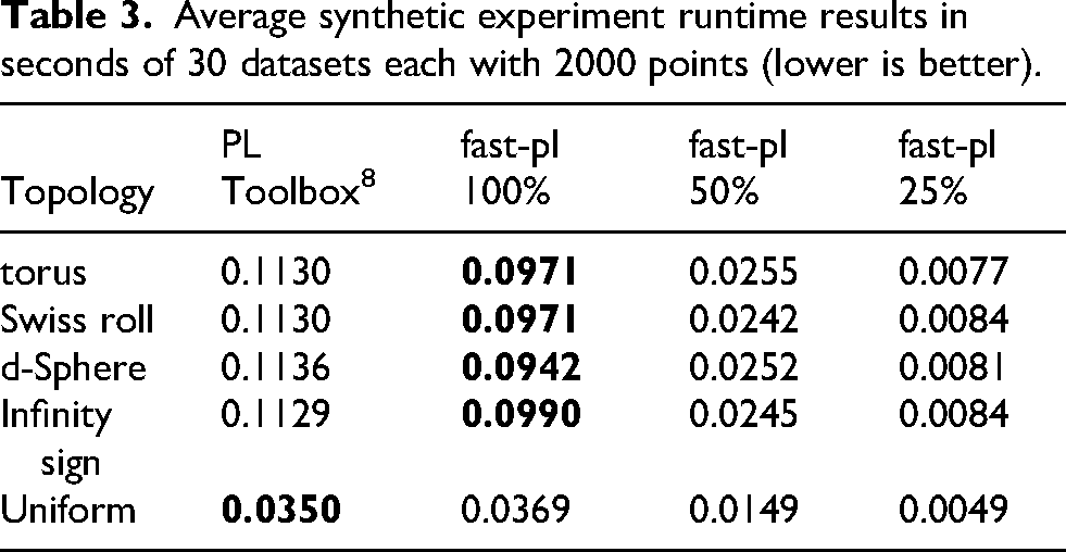
To experimentally validate the performance of the new plane sweep algorithm against the original exact algorithm from Bubenik et al. 8 as the number of points in the topology grows, point clouds of various topologies were generated. For this experimental evaluation, the proposed work is implemented using a Rust package created by the authors named “fast-pl.” This was done to compare the algorithm’s time bound while eliminating as many variables as possible. It allows us to change any variable in the dataset, including noise levels. This gives us the ability to quantify if any of these variables affect the relative run time between the two algorithms. We included different topologies to see if this would have any effect on the runtimes as well. Point clouds for the torus, Swiss roll, d-sphere, and infinity sign were generated. Additionally, a dataset of uniformly distributed birth-death pairs was generated to mimic how the original algorithm’s time-bound growth was quantified by Bubenik et al. 8
For each type of topology, datasets were generated from 100 to 10,000 points in steps of size 100. Some datasets stopped before 10,000 points because the compute resources available did not have enough memory to generate the dataset properly. When generating datasets of uniform persistence pairs, the number of persistence pairs used goes from 100 to 10,000 with steps of 100. For each set of persistence pairs, 30 samples were generated, for a total of 3000 datasets per type. The TaDAsets package 23 was used to generate the datasets. The parameters used to generate each type of topology can be seen in Table 1.
TaDAsets parameters.

The same datasets were run through our implementation as well as the PL Toolbox implementation
8
(the original and standard method used to compute PL). We ran our code, fast-pl, allowing for a variable number of top-

Runtime comparison on the synthetic torus dataset.

Runtime comparison on the synthetic Swiss roll dataset.

Runtime comparison on the synthetic d-sphere dataset.

Runtime comparison on the synthetic infinity sign dataset.

Runtime comparison of uniformly distributed persistence pairs.
Classification performance between algorithms.

Average synthetic experiment runtime results in seconds of 30 datasets each with 2000 points (lower is better).
Botnet experiments
We tested our algorithm against the previous best using a real-world botnet dataset. This was chosen because this problem is an active field of research in cybersecurity and TDA-PL has shown promise in being able to classify network traffic. 7 Therefore, as computer network analysis is a field that has shown interest in using TDA and botnet detection is an open problem in that field, botnet detection was chosen to confirm the algorithms in a real-world practical setting. 24 There are many ways to apply TDA to real-world problems for computer network analysis. This showcases one way of how to use the provided algorithms to perform data analysis on an applicable, complex, real-world problem. It is not the goal of this work to provide state-of-the-art results in botnet detection but to show the potential performance gains of the newly introduced algorithms in a real-world, practical setting. The data pipeline and machine learning metrics provided are in line with standard practices in the field of computer network analysis.
Botnet detection is a more complex pipeline that uses PL and has found success in financial time series classification and prediction.2,3 By using a real-world dataset, we can validate if the success of the new algorithm in the synthetic experiments holds for use cases where it would be used in practice. It should be noted that the previous best approximation algorithm was rewritten in Python in these experiments to work with existing processing pipelines.
Preprocessing and feature engineering are critical steps for all time series efforts. For these experiments, Python 3.8 with NumPy and pandas were used. Ripser was the TDA package used for the Vietoris-Rips filtration, as it was shown by Otter et al. 25 to be the best for the task and has a Python implementation using the work of Tralie et al. 26 We used representative pattern matching (RPM) for the classification of the resulting data from the TDA stage.
Using the datasets described below, we treat each pcap packet capture as a set of points. Given these ordered sequences of points, the pipeline does the following to transform a multi-attribute time series into a univariate time series. First, it separates the time series into ordered sets of equal size determined by a user-defined window size,
We must convert each of these landscapes into a single value that can represent the overall homology of the window and can be compared to other windows. This is accomplished using the
The experiments used two different machines: a high-end desktop (HEDT) and a multiuser server. All other users were logged off the multiuser system for all experiments containing relative speedup results, apart from user experimenting. This was done to minimize the experimental noise introduced into the results from other users’ activities. Times were captured by taking the wall time difference before and after the TDA step only (dimensionality reduction stage). This was done to demonstrate the time savings from changing the algorithms used. The exact specifications of each machine are given in Table 4.
Hardware specifications.

HEDT: high-end desktop; CPU: central processing unit; OS: operating system.
We examined two botnet datasets. The first is ISCX Botnet 2014 from the University of New Brunswick Canadian Institute for Cybersecurity. 27 This dataset has the three main attributes of a good dataset: generality, realism, and representativeness. They accomplished this by including many types and manifestations of botnets from multiple data collection points. The data format is multiple pcap files. Having access to the raw pcap files greatly increases the different types of techniques that can be evaluated on the dataset as pcap is the industry standard for network capture and replay. The result is a greater number of people who can use the dataset to evaluate their algorithm, making it easier for the dataset to become a standard for evaluation.
The training dataset contains seven different botnets. Each of which is either IRC, HTTP, or P2P, with 43.92% of the traffic being malicious. The testing set contains 16 different botnets. Each of these botnets is one of the previously seen types from the training dataset, with 44.97% being malicious. All the original botnet types appear in the testing dataset. This enables one to test the previously mentioned different types of generalizations for the model in question.
Preprocessing
The following preprocessing was done on the dataset:
pcap to CSV and feature selection using Argus sample labeling in python feature engineering in Python test/train split CSV to JSON in Python
Feature selection using Argus
The ISCX dataset comes as pcap files, which means that feature selection is needed. Feature selection is done using openargus. The features are given in Table 5. These features are chosen out of the possible 145 because not all the available features are thought to be helpful in the botnet detection problem. 28 These are very similar to the features that are used by Homayoun et al. 28 The reason for the difference is that some of the features never changed in value in the ISCX botnet dataset and thus added no information. If these features in the dataset were to change, it might be worthwhile to add them back. More feature extraction could be done to the dataset than what was done here.
Features extracted from the ISCX 2014 Botnet dataset.

The output from open Argus is customizable to most formats; CSV is used here. The source IP, destination IP, and port were not used during classification to enable better generalization to new networks.
Time-series split
The input to RPM needs to be formatted as a collection of time series. Thus, we must decide how to group the data and where to split the different samples. We decided to order all the data sequentially according to time and then split the data into 500 sample chunks with no overlap between any chunks. This number was chosen as it was the minimum to allow for patterns to be found. This results in having the maximum number of samples possible for testing and training and ensuring that botnets are detected as soon as possible if deployed in a real-time system.
Data labeling
As a result of the data provided by the ISCX botnet being provided as pcap files, the data is unlabeled. ISCX provides a list of the malicious IPs seen in the network capture. The data is labeled so that if there is a bad connection in the sample chunk, then the entire chunk is labeled as malicious. If there is no bad connection in the chunk, then the chunk is labeled as benign.
Feature engineering
Extra feature engineering was done on top of the initial feature selection from open Argus. The data was read into a Python file as a CSV, then min-max normalization and one-hot encoding are done using pandas and NumPy. Then, features with all NaN values are removed to shrink the dataset’s size, as these features provided no additional information for the model. Lastly, the data is exported as a CSV.
Test/train split
The testing and training datasets are manipulated in a subset of the experiments. If there is manipulation of the testing and training data in an experiment, the following done. A random value between 0 and 1 is assigned to each sample chunk. If the value is greater than a user-defined threshold value, then that value is assigned to the training set. If it is less than the value, it is assigned to the testing set. This was only done when the original training and testing datasets were not used, and the original training dataset was split into new training and testing sets.
CSV to JSON
The final stage of the data preprocessing pipeline is a conversion from CSV to JSON. This is done for compatibility reasons to use our implementation of RPM. The conversion is done using pandas in Python and is provided along with the other source code on http://github.com/tph5595/.
Plane sweep algorithm analysis validation
The purpose of these experiments is to see if the plane-sweep algorithm from the “Plane-Sweep landscape generation” subsection performed better than the original approximation algorithm. 8
Method
A grid search is done using the ISCX Botnet 2014 dataset on both algorithms to test this. The grid search is performed on the window size (5–40 with a step size of 5) and the max Rips radius (1–5 with a step size of 1). Experiments were run with the persistence pair filtering step, keeping every birth-death pair and only keeping the top
Algorithm runtime (seconds) at the 95% confidence level.

Mean weighted MCC and weighted F1.

Generalization
The initial findings on the ISCX Botnet 2014 dataset were underwhelming compared to the success achieved using TDA on other datasets.
2
The result was a weighted F1 of
Max metrics on different datasets.

Training the model on this new dataset increased the weighted F1 to
Experiments were conducted to quantify the effect of the loss of information caused by using TDA for time series dimensionality reduction for botnet classification. The model was trained and tested on the ISCX training dataset. The result was that the model was able to achieve a weighted F1 of 0.997 and a weighted MCC of 0.993 (only one misclassified example). This can be seen in Table 8 which shows TDA’s ability to reduce the dimensionality of the botnet time series data from 26 dimensions to one with minimal loss of information. This instills confidence that univariate time series analysis techniques can be used on multivariate data. There is a greater understanding of how to analyze univariate than multivariate time series data—thus, opening the door for these techniques to be used on multivariate time series data. Further work should be done with TDA with other time series analysis models, techniques, and features to determine the best combination.
It should be noted that the best parameters for all the different experiments in this section were the same: a window size of 20 and a maximum rip radius of 4. There is no reason this should have been the case, as different training sets were created for all different experiments. Therefore, it is logical to assume that some attribute is inherent to the network that is causing this. This helps with training various TDA implementations on the same network, as it seems only a single search for the correct parameters might be needed.
Software details
The software used for the experiments in this article is available on GitHub in Rust at http://github.com/tph5595/fast-pl. The project is also available in a pip package available at the Python package index at https://pypi.org/project/fast-pl-py/. It can be installed using Python 3.8 and pip, using the name fast–pl–py. The methods allow for the algorithms presented to be easily imported and used with existing data analysis programs written in these languages. Additionally, examples are included at http://github.com/tph5595 which use the software in real-world settings.
Conclusion
We have shown that PLs can be computed significantly faster than previously possible. This was done by gaining two independent insights on the geometric structure of the problem. First, by using a preprocessing step to filter out birthdeath pairs from the PL calculation that cannot appear in the top-
Future work should be done to optimize the code, and rewriting in a lower language may be useful in some circumstances. Additionally, work still needs to be done with PL to ensure that it can be used to its fullest potential in the face of noise and when integrated into complex processing pipelines like those seen in time series analysis.
Footnotes
Funding
The author(s) disclosed receipt of the following financial support for the research, authorship, and/or publication of this article: This research received no specific grant from any funding agency in the public, commercial, or not-for-profit sectors.
Declaration of conflicting interests
The author(s) declared no potential conflicts of interest with respect to the research, authorship, and/or publication of this article.