Sage Journals: Discover world-class research

Abstract

This study introduces significant improvements in the construction of deep convolutional neural network models for classifying agricultural products, specifically oranges, based on their shape, size, and color. Utilizing the MobileNetV2 architecture, this research leverages its efficiency and lightweight nature, making it suitable for mobile and embedded applications. Key techniques such as depthwise separable convolutions, linear bottlenecks, and inverted residuals help reduce the number of parameters and computational load while maintaining high performance in feature extraction. Additionally, the study employs comprehensive data augmentation methods, including horizontal and vertical flips, grayscale transformations, hue adjustments, brightness adjustments, and noise addition to enhance the model's robustness and generalization capabilities. The proposed model demonstrates superior performance, achieving an overall accuracy of 99.53%∼100% with nearly perfect precision, recall of 95.7%, and F1-score of 94.6% for both “orange_good” and “orange_bad” classes, significantly outperforming previous models which typically achieved accuracies between 70% and 90%. While the classification performance was near-perfect in some aspects, there were minor errors in specific detection tasks. The confusion matrix shows that the model has high sensitivity and specificity, with very few misclassifications. Finally, this study highlights the practical applicability of the proposed model, particularly its easy deployment on resource-constrained devices and its effectiveness in agricultural product quality control processes. These findings affirm the model in this research as a reliable and highly efficient tool for agricultural product classification, surpassing the capabilities of traditional models in this field.

Keywords

Deep convolutional neural network MobileNetV2 data augmentation feature extraction depthwise separable convolutions linear bottlenecks inverted residuals image classification

Introduction

Image recognition is a crucial research area in artificial intelligence and machine learning, with broad applications spanning healthcare,^1,2 security,³ transportation, and e-commerce.^4,5 Recent advancements in deep learning models have led to significant breakthroughs, particularly with deep convolutional neural networks (DCNNs).^6,7 DCNNs are a type of deep artificial neural network specifically designed to process grid-structured data,^8,9 such as images.⁹ They consist of multiple convolutional layers, activation layers, pooling layers, and fully connected layers. Convolutional layers perform convolution operations to extract local features from images,⁹ pooling layers reduce the spatial dimensions of these features, and fully connected layers integrate the information for classification.^10,11 Some prominent DCNN models include AlexNet, VGGNet, GoogLeNet, and ResNet.^12,13 AlexNet was one of the first models to achieve significant success in the ImageNet competition, known for its depth and the use of ReLU to accelerate training.^14,15 VGGNet is noted for its simple yet effective architecture, utilizing small 3 × 3 convolutional layers. GoogLeNet introduced the Inception module, a structure that allows the model to learn features at multiple resolutions. ResNet addresses the vanishing gradient problem in deep networks through the use of skip connections, enabling more efficient feature learning.¹⁶ Besides DCNNs, other models such as recurrent neural networks (RNNs) and long short-term memory (LSTM)¹⁷ networks are widely used for action recognition in videos, medical image sequence analysis, and other applications requiring sequential data processing. Generative adversarial networks (GANs)¹⁸ have also brought about many groundbreaking applications, such as generating images from text, enhancing image quality, and creating synthetic image samples for model training.¹⁹

Machine learning has brought about numerous breakthroughs in image recognition, thanks to its ability to learn from large datasets and automatically extract features. In healthcare, deep learning models assist in detecting pathologies from X-ray,^1,20 MRI,² and CT³ scan images with high accuracy. For example, these models can early detect signs of cancer, cardiovascular diseases, or brain disorders,^21,22 aiding doctors in diagnosis²³ and treatment.^24,25 Recognizing and classifying cells from microscopic images²⁶ helps automate research processes and disease detection.^27,28 These models can classify different types of cells, detect abnormal or infected cells, and analyze cell samples for studying complex diseases.²⁹ In security, facial recognition systems are deployed at airports, shopping centers, and public places to enhance security. Machine learning aids in recognizing faces from images and videos, comparing them with databases to identify individuals and detect persons of interest. It also helps detect unusual behaviors from surveillance videos, providing timely alerts for security risks. Deep learning models can analyze human behavior in monitored areas, identifying suspicious activities such as intrusion, violence, or unusual actions. In transportation, automatic license plate recognition systems help manage traffic, automate toll collection, and detect traffic violations. Machine learning extracts and recognizes license plates from images, comparing them with databases to identify violators or vehicles of interest. Image recognition models assist self-driving cars in detecting and recognizing objects, traffic signs, and pedestrians. Machine learning enables self-driving cars to understand and interact with their surroundings, ensuring safe and efficient navigation. In e-commerce, image recognition technology helps customers search for products by taking pictures or uploading images of desired products. Machine learning identifies product features from images and searches for similar items in the database. Automatic product classification from images helps manage inventory and display products on online shopping platforms. Machine learning classifies products based on features such as color, shape, size, and other attributes.³⁰ Image recognition is a promising field that has seen many breakthroughs due to deep learning models. These advancements not only improve the performance of recognition systems but also open up new applications in healthcare, security, transportation, and e-commerce. Machine learning continues to play a crucial role in enhancing the quality of life and creating smarter solutions for challenges in daily life and industry.^31,32 Image recognition is also bringing significant improvements to agriculture, enhancing efficiency and production quality.³³ By applying this technology, farmers can monitor and manage crops more effectively, from early disease detection,³⁴ weed management, and irrigation optimization to product sorting and quality control.^35,36 In processing plants, image recognition is used to sort agricultural products based on shape, size, and color, removing substandard products and ensuring only the best ones reach the market. Additionally, image recognition helps inspect product quality during production, detecting issues early and minimizing waste. In canned fruit production, this technology can inspect each fruit to ensure there are no damaged or diseased ones. These applications not only increase productivity and profitability but also contribute to environmental protection and sustainable agriculture development. In the future, with the continuous advancement of artificial intelligence and machine learning, image recognition will continue to play a key role in modernizing and improving the efficiency of the agricultural industry.

To provide a comprehensive background on fruit classification using deep learning, this study builds on recent advancements in the field. Previous work has explored various deep learning models and techniques for agricultural product classification. For instance, the MobileNetV2 architecture has been employed in fruit image classification using deep transfer learning techniques, demonstrating significant improvements in classification accuracy and efficiency.³⁷ Similarly, soybean classification has been enhanced using a modified Inception model, showcasing the effectiveness of transfer learning for agricultural applications.³⁸ Further advancements have been made in corn seed disease classification by leveraging MobileNetV2 with feature augmentation and transfer learning, which highlights the importance of feature extraction in improving model performance.³⁹ In addition, research on the adaptability of deep learning models has provided insights into how various datasets and strategies can impact fruit classification accuracy.³⁷ The use of convolutional neural networks (CNN) has also been applied to seed classification systems, offering a foundation for CNN-based approaches in agricultural classification tasks.³⁸ Moreover, techniques for enhancing image annotation in fruit classification have demonstrated the importance of precise labeling in improving the robustness of deep learning models.³⁹ By building on these studies, the current work applies MobileNetV2 and data augmentation techniques to orange quality classification, while also addressing the challenges of limited datasets and variability in real-world conditions. This approach aligns with the latest contributions in deep learning for agricultural applications and further advances the field by optimizing classification for orange quality.

While significant progress has been made in using deep learning models for fruit classification, several limitations remain in existing research. Many previous studies have focused on architectures such as ResNet or VGGNet, which, although effective, often require substantial computational resources, limiting their applicability in real-time, resource-constrained environments such as agricultural fields. Furthermore, these models often struggle with generalizing well to real-world conditions where variations in lighting, angle, and image quality are common. Data augmentation techniques have been applied, but many studies rely on basic augmentations, limiting the model's robustness and ability to handle diverse conditions. This study addresses these gaps by leveraging the lightweight and efficient MobileNetV2 architecture, which allows for deployment on mobile and embedded devices, making it highly suitable for real-time applications in agriculture. Additionally, we incorporate a more comprehensive set of data augmentation techniques, such as hue adjustment, brightness variation, and noise addition, to enhance the model's robustness and generalization capabilities. By addressing these limitations, this study presents a novel and practical solution for agricultural product classification, particularly for oranges, setting a new benchmark for model performance and applicability in real-world scenarios.

This study introduces significant improvements in the construction of DCNN models for classifying agricultural products, specifically oranges, based on their shape, size, and color. Utilizing the MobileNetV2 architecture, this research leverages its efficiency and lightweight nature, making it suitable for mobile and embedded applications. Key techniques such as depthwise separable convolutions, linear bottlenecks, and inverted residuals help reduce the number of parameters and computational load while maintaining high performance in feature extraction. Additionally, the study employs comprehensive data augmentation methods, including horizontal and vertical flips, grayscale transformations, hue adjustments, brightness adjustments, and noise addition to enhance the model's robustness and generalization capabilities. The MobileNetV2 architecture is chosen for its balance between performance and computational efficiency, making it ideal for deployment on devices with limited resources. Depthwise separable convolutions break down the standard convolution process into two simpler operations, significantly reducing the computational cost. Linear bottlenecks and inverted residuals help in preserving information through narrow layers and ensuring efficient feature propagation through the network. Comprehensive data augmentation techniques play a crucial role in improving the model's robustness. Horizontal and vertical flips create a diverse set of training samples by flipping the images along different axes, simulating various viewing angles. Grayscale transformations convert images to grayscale, enabling the model to focus on texture and shape features rather than color, thereby enhancing its generalization ability. Hue and brightness adjustments simulate different lighting conditions, allowing the model to recognize oranges under various lighting scenarios. Adding random noise to images increases the model's robustness by training it to handle imperfections and variations in image quality. The proposed model demonstrates superior performance, with a total of 637 predictions and 634 correct predictions, resulting in an overall accuracy of 634/637. This equates to an accuracy of 99.53%∼100% with nearly perfect precision, recall, and F1-score for both “orange_good” and “orange_bad” classes. This significantly outperforms previous models, which typically achieved accuracies between 70% and 90%. The confusion matrix analysis reveals high sensitivity (true positive rate) and specificity (true negative rate), with minimal misclassifications, demonstrating the model's reliability. The study also empresentasizes the practical applicability of the proposed model. The lightweight nature of MobileNetV2 allows for easy deployment on mobile devices and embedded systems, making it practical for use in the field. The model's high accuracy and robustness make it an effective tool for real-time quality assessment and sorting of agricultural products, ensuring only the best products reach the market. Furthermore, the model's scalability and efficiency make it adaptable for other types of agricultural products, providing a versatile solution for various classification tasks. In conclusion, this study's findings affirm the proposed DCNN model as a reliable and highly efficient tool for agricultural product classification, surpassing the capabilities of traditional models in this field. By leveraging advanced techniques in deep learning and data augmentation, the model not only improves classification accuracy but also enhances the practical applicability of machine learning in agriculture. Future work could explore further optimizations and adaptations of the model for a broader range of agricultural products and real-world deployment scenarios.

This study presents several novel contributions to the field of orange classification, setting it apart from previous research: ➢

Use of MobileNetV2 architecture: While previous studies have employed various deep learning architectures for fruit classification, our study leverages the MobileNetV2 architecture for the first time in orange classification, known for its computational efficiency and suitability for mobile and embedded devices. This is particularly important for real-time quality control applications in resource-constrained environments, such as agricultural fields.

➢

Advanced data augmentation techniques: We incorporated a comprehensive set of data augmentation techniques, including hue adjustments, brightness variations, grayscale transformation, and noise addition. These techniques significantly improve the model's robustness by allowing it to generalize well across different conditions, such as varying lighting and image quality, which is a common challenge in agricultural product classification.

➢

High precision and generalization: Our model achieved nearly perfect classification performance, with an accuracy of 99.53%, precision of 99–100%, and F1-scores nearing 1.00. This performance outperforms traditional models that typically reach 70–90% accuracy, setting a new benchmark for classification models in this domain.

➢

Scalability and practical application: The lightweight design of MobileNetV2 allows for easy deployment on mobile and embedded systems, making the model highly scalable and practical for real-world applications. This makes it ideal for farmers and agricultural industries, where quick, reliable assessments are critical for maintaining product quality.

These contributions demonstrate the significant advancements this study brings to both the field of deep learning and its practical application in agricultural product classification.

DCNN algorithm model

CNN algorithm model

CNNs²⁵ are a type of deep neural network specifically designed to process grid-like data structures such as images. These networks consist of multiple convolutional layers and pooling layers, combined with fully connected layers to efficiently extract and classify features from input data.^40,41 In a convolutional layer, the network performs a convolution operation between the input matrix and a filter, mathematically represented as follows⁴²:

(I * K) (i, j) = \sum_{m} \sum_{n} I (i + m, j + n) . K (m, n)

(1)

where I is the input matrix, K is the filter, and (i, j) are the coordinates of the output matrix. Then, the activation layer introduces nonlinearity into the model using the rectified linear unit (ReLU) function defined in equation (2):

f (x) = max (0, x)

(2)

The pooling layer, often employing the max pooling method, reduces the spatial dimensions of the data while retaining important features, described in equation (3):

P (i, j) = max {I (i + m, i + n) | 0 \leq m, n < s

(3)

in which P is the output matrix and s is the size of the pooling region. In the fully connected layer, neurons are fully connected to all activations in the previous layer, transforming the input according to equation (4):

y = W x + b

(4)

where W is the weight matrix, x is the input vector, b is the bias vector, and y is the output vector. Finally, in classification tasks, the output layer uses the softmax function to convert score values into probabilities, as given in equation (5).

σ (z)_{i} = \frac{e^{z_{i}}}{\sum_{j} e^{z_{j}}}

(5)

where z is the input vector of the softmax function.

CNNs have a wide range of applications. They are used in image recognition tasks such as facial recognition, license plate detection, and object detection in various images. In image classification, CNNs classify images into different categories, which are useful in medical diagnosis, animal classification, and many other fields.⁴³ For image segmentation, CNNs identify and segment specific regions within an image, which is crucial for precise tasks like medical diagnosis. Additionally, computer vision applications in autonomous vehicles, quality control in manufacturing, and intelligent robots use CNNs to analyze and understand image data, making them powerful tools in image processing and analysis across various domains.

DCNN algorithm model

The differences between DCNN and CNN are well known and include the following³⁶: ➢

DCNNs are an extended version of CNNs,⁴⁴ with the main difference being in the depth and the ability to learn more complex features from the data. While CNNs typically have 3–10 convolutional and pooling layers combined with one or two fully connected layers, DCNNs can include from 10 to hundreds of layers. This allows DCNNs to learn higher-level and more abstract features, whereas CNNs mainly focus on simple to medium-level features.

➢

DCNNs have a superior ability to learn features due to the larger number of layers, enabling them to process and recognize more complex features from the input data.^45,46 The initial layers in DCNNs learn low-level features, the subsequent layers learn medium-level and higher features, and the deepest layers learn high-level features such as complex shapes and relationships between objects. In contrast, CNNs can only learn simple features like edges and corners.

➢

DCNNs also outperform CNNs in complex tasks.^47,48 They are often used in applications requiring high accuracy, such as object recognition in natural images, medical image segmentation, and complex recognition and classification systems. On the other hand, CNNs are more suitable for simple to medium tasks like handwritten character recognition, basic facial recognition, and simple image classification.

➢

DCNNs require more computational resources, including powerful CPUs/GPUs and more memory for processing, leading to longer training times and the need for more data to achieve optimal performance.^49,50 In contrast, CNNs require fewer resources and have shorter training times, making them suitable for devices with limited computational capabilities and real-time applications.

➢

DCNN applications include autonomous vehicles, medical image segmentation, and security surveillance systems, while CNNs are widely used in handwritten character recognition, facial recognition, and simple image classification.⁵¹

In summary, DCNNs are a deeper and more extended form of CNNs, with the ability to learn more complex features, higher performance, and accuracy in complex tasks, but they require more computational resources.

Performance evaluation model

While accuracy provides a simple overview of the model's performance by indicating the percentage of correctly classified samples, it is not always sufficient, especially in cases with imbalanced data. Therefore, alongside accuracy, we have also reported precision, recall, and F1-score to offer a more comprehensive evaluation of the model's classification ability. These additional metrics help capture the model's performance in distinguishing between different classes more effectively, particularly when dealing with imbalanced datasets.

Accuracy

Accuracy is a commonly used metric in classification tasks, representing the percentage of correctly classified samples. While it provides a general overview of the model's performance, it can be misleading with imbalanced datasets, as it does not distinguish between different classes. In such cases, metrics like precision, recall, and F1-score offer a more comprehensive evaluation of the model's classification ability. The formula for accuracy is given by

A c c u r a c y = \frac{Number of True samples (T P + T N)}{Total number of samples (T P + T N + F P + F N)}

(6)

in which TP (true positive) is the number of positive samples correctly classified, TN (true negative) is the number of negative samples correctly classified, FP (false positive) is the number of negative samples incorrectly classified as positive, and FN (false negative) is the number of positive samples incorrectly classified as negative.

Precision

Precision measures the percentage of true positive predictions out of all positive predictions (true positives and false positives). It is particularly useful in cases where false positives carry significant consequences, such as in medical diagnosis or fraud detection. Precision is especially important in imbalanced datasets but should be considered alongside recall for a comprehensive evaluation.

Precision = \frac{True Positives (TP)}{True Positives (TP) + False Positives (FP)}

(7)

in which TP (true positives) are the number of positive samples correctly predicted and FP (false positives) are the number of negative samples incorrectly predicted as positive.

Recall

Recall, or sensitivity, measures a model's ability to correctly identify positive samples. It is calculated as the ratio of true positives to the total number of actual positive samples (true positives + false negatives). High recall indicates that the model misses few positive cases, which is crucial in applications like medical diagnosis or identifying dangerous objects:

Recall = \frac{True Positives (TP)}{True Positives (TP) + False Negatives (FN)}

(8)

in which true positives (TP) are the number of images containing the object that the model correctly identifies and false negatives (FN) are the number of images containing the object that the model fails to identify.

F1-score

The F1-score is the harmonic mean of precision and recall, providing a balanced measure of a model's performance, particularly in imbalanced datasets. It is useful in evaluating a model's ability to correctly classify objects while minimizing errors. The F1-score is calculated based on precision and recall:

F 1 Score = 2 \times \frac{Precision \times Recall}{Precision + Recall}

(9)

in which precision is the ratio of the number of true positive results (true positives) to the total number of results predicted as positive by the model (true positives + false positives).

Precision = \frac{True Positives}{True Positives + False Positives}

(10)

In which recall is the ratio of the number of true positive results (true positives) to the total number of actual positive samples (true positives + false negatives).

Recall = \frac{True Positives}{True Positives + False Negatives}

(11)

A high F1-score indicates that the model has a good balance between precision and recall, meaning it not only correctly identifies objects but also misses few of them. This is very important in image recognition applications.

Confusion matrix

The confusion matrix is a tool used to evaluate the performance of a classification model by showing the number of correct and incorrect predictions for each class. It provides a detailed analysis of how the model classifies data as shown in Table 1. In a binary classification problem, it represents actual and predicted values in a square matrix format:

Table 1.

Square matrix with rows and columns representing the classes.

	Predicted positive	Predicted negative
Actual positive	True positive (TP)	False negative (FN)
Actual negative	False positive (FP)	True negative (TN)

Key components: –

True positive (TP): The number of samples predicted as positive and is actually positive

–

False positive (FP): The number of samples predicted as positive but is actually negative

–

False negative (FN): The number of samples predicted as negative but is actually positive

–

True negative (TN): The number of samples predicted as negative and is actually negative

The confusion matrix is a powerful tool for detailed evaluation of the performance of image recognition models. It provides crucial information for calculating metrics such as precision, recall, accuracy, and F1-score, thereby aiding in the optimization and improvement of the model.

Receiver operating characteristic curve and area under the curve

The Receiver operating characteristic (ROC) curve is a graphical tool used to evaluate a binary classification model's performance by plotting the relationship between the true positive rate (TPR) and false positive rate (FPR) across different thresholds. The area under the curve (AUC) quantifies this performance, with values ranging from 0 to 1, where AUC = 1 indicates perfect classification and AUC = 0.5 reflects random guessing. The ROC curve and AUC are essential in assessing a model's ability to distinguish between classes, particularly in fields like medical diagnosis, security, and transportation.

Mean squared error

Evaluating the performance of machine learning models is crucial to ensure the accuracy and effectiveness of classification algorithms in image recognition. A common metric is mean squared error (MSE), which measures the average error between predicted and actual values by averaging the squared errors.

M S E = \frac{1}{n} \sum_{i = 1}^{n} {(y_{i} - {\hat{y}}_{i})}^{2}

(13)

In image recognition, MSE evaluates model performance by comparing predicted and actual class labels, as well as object positions and sizes in detection tasks. While MSE is simple to calculate and sensitive to large errors, it can be overly sensitive and is not directly comparable across models with different scales.

Data model

The dataset used for this study consists of 9577 images of oranges. These images were sourced from various locations to ensure diversity in the dataset, including differences in lighting, ripeness, and orange varieties. The dataset was divided into two classes:

“orange_good”: Represents high-quality oranges that meet the criteria for being visually appealing, well-formed, and free from defects

“orange_bad”: Represents lower-quality oranges that exhibit deformities, discoloration, or damage, such as bruises or scars

The dataset was split into training, validation, and test sets in the ratio of 70:20:10 to ensure that the model could generalize well across unseen data.

Orange classification

Data preprocessing

Data preprocessing is a crucial step in preparing data for the model training process. This procedure ensures that the input data is thoroughly prepared and optimized for training, thereby enhancing the effectiveness and accuracy of predictions. The detailed steps in the preprocessing procedure are as follows: ➢

Auto-orient: Auto-orient is the process of automatically adjusting the orientation of images to eliminate inconsistencies. Images collected from various sources may have different orientations, such as some images being sideways or upside down. Auto-orient ensures that all input images have the same orientation, which is essential for the model to consistently detect and recognize features. This also helps eliminate unwanted distortions due to directional differences, increasing the model's accuracy.

➢

Resize: Images are resized to 224 × 224 pixels. This size is chosen because it is a common standard in many computer vision models, large enough to retain important details but small enough to minimize memory and computational requirements. Resizing helps standardize the input data, making it easier for the model to learn and process. If images have inconsistent sizes, the model may struggle to detect features consistently.

➢

Data integration: Data integration is the process of combining multiple datasets to increase the diversity and richness of the training data. Datasets from various sources are carefully selected to ensure the representativeness and diversity of the training samples. This helps the model learn from various scenarios and cases, enhancing its generalization ability. For example, data may include images of oranges from different growing regions, under different lighting conditions, and at various ripeness stages.

➢

Data cleaning: Data cleaning involves removing images that may cause noise, such as blurry, defective, or irrelevant images. Blurry or defective images may contain little useful information and reduce the model's accuracy. Removing irrelevant images helps minimize negative impacts on the training process, ensuring the model learns only from high-quality data. This process includes inspecting and eliminating images with technical errors, such as distortion, blurriness, or improper cropping.

➢

Data labeling: Data labeling is the step of categorizing images into specific groups, in this case, “orange_good” and “orange_bad.” This helps the model clearly distinguish between good and bad orange samples. The labeling process must be done carefully and accurately, as incorrect labels can lead to incorrect learning and predictions. The criteria for labeling include color, shape, and skin condition of the oranges, as defined in previous sections.

These preprocessing steps ensure that the input data is thoroughly prepared and optimized for the model training process. Auto-orient helps standardize image orientation. Resize adjusts image size to a uniform standard. Data integration increases data diversity. Data cleaning removes unnecessary and noisy elements. Data labeling clearly categorizes the training samples. These steps not only enhance the effectiveness of the training process but also ensure that the model can make accurate and reliable predictions.

Augmentations

Data augmentation is an important technique in machine learning, particularly in computer vision tasks, aimed at enhancing the diversity of training data and improving the model's performance. The applied data augmentation methods include flip, grayscale, hue, brightness, and noise. ➢

Flip includes two types both horizontal flip and vertical flip. Horizontal flip mirrors the image horizontally, creating a reflection of the original image, helping the model learn horizontal transformations, thereby recognizing symmetry and other features in the data. Vertical flip mirrors the image vertically, similar to horizontal flipping, aiding the model in learning vertical transformations and recognizing features from different perspectives.

➢

Grayscale applies grayscale to 25% of the images, enabling the model to learn features independent of color, focusing on structure and shape. Hue adjusts the hue of the images within a range of −25° to +25°, making the model more adaptable to color variations, thus distinguishing objects even when colors change. Brightness adjusts the brightness of the images within a range of −25% to +25%, allowing the model to learn features under varying lighting conditions, enhancing recognition in diverse lighting environments.

➢

Noise adds noise to up to 1.96% of the image pixels, making the model more robust and capable of learning important features even when data is noisy. Adding noise ensures the model is less affected by disruptive elements in real-world data, such as dirt, shadows, or defective pixels.

After performing data preprocessing and augmentation, the complete dataset of 9577 images is split into a 70-20-10 ratio, with 70% of the data used for model training, 20% for validation, and 10% for final testing. Applying preprocessing and data augmentation methods ensures that the training dataset is highly diverse, allowing the model to learn features from various scenarios and conditions, thereby improving the model's accuracy and generalization capability as shown in Figure 1.

Figure 1.

Sample images representing the dataset.

Orange detection

The dataset used in this study consists of 9577 images of oranges, divided into two classes: “orange_good” and “orange_bad.” The distribution includes 4532 images labeled as “orange_good” and 5045 images labeled as “orange_bad.”

The images were collected from various sources, ensuring diversity in lighting, angles, and conditions to simulate real-world scenarios. This dataset reflects different stages of ripeness and various conditions under which oranges are grown and harvested. Each image was manually labeled based on visible criteria such as color, texture, and defects.

The dataset was divided into training (70%), validation (20%), and testing (10%) sets to ensure that the model's performance is accurately evaluated. The images were resized to 224 × 224 pixels for input into the MobileNetV2 architecture, optimizing both accuracy and computational efficiency. The average image size in the orange detection dataset is 310 × 282 pixels, as shown in Figure 2.

Figure 2.

Chart showing the distribution of aspect ratios of oranges.

Dividing the dataset according to these proportions ensures that the model is trained with a sufficiently large amount of data while having adequate validation and test sets to evaluate the model's performance and generalization capability. The average image size of 310 × 282 pixels provides sufficient resolution to detect and classify the necessary features of the oranges during the detection process, as illustrated in Figure 3.

Figure 3.

Common shapes of oranges.

Definition and criteria for evaluating orange quality

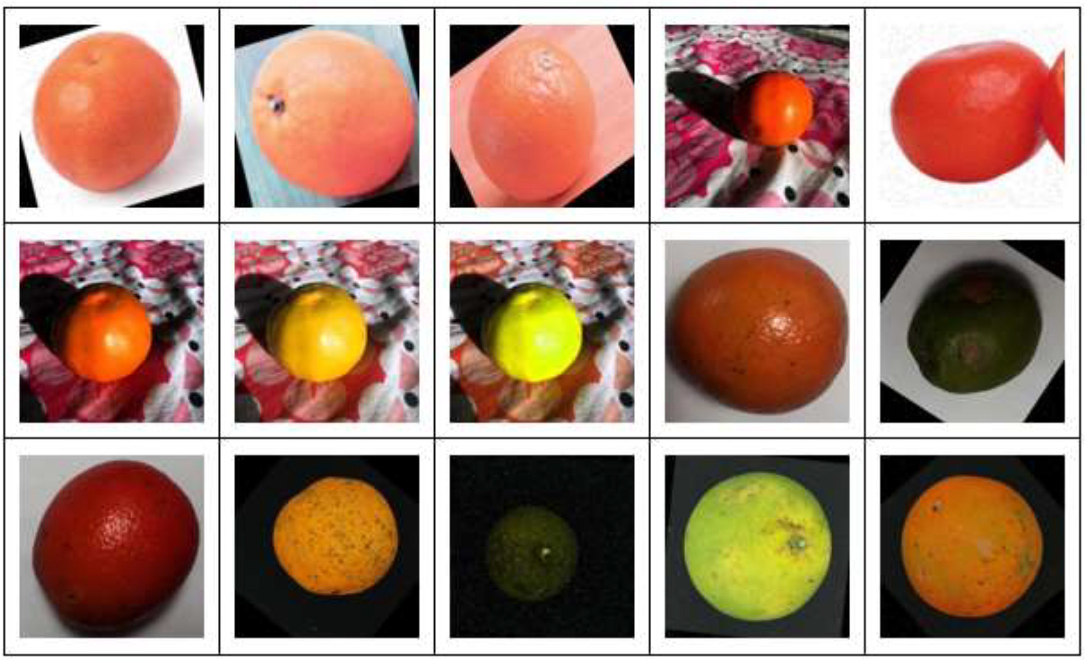
The quality of oranges can be assessed based on specific criteria related to color, shape, and skin condition. A good orange typically has a uniform color, which can be either orange or green with a bright, vibrant hue, without any signs of fading, as shown in Figure 4. The shape of a good orange is usually round and even, without deformities or dents, indicating that the orange has developed under favorable conditions without external impacts. A good orange's skin is smooth, free of bruises, scars, or cracks, reflecting that the orange is free from pests or damage due to mechanical effects.

Figure 4.

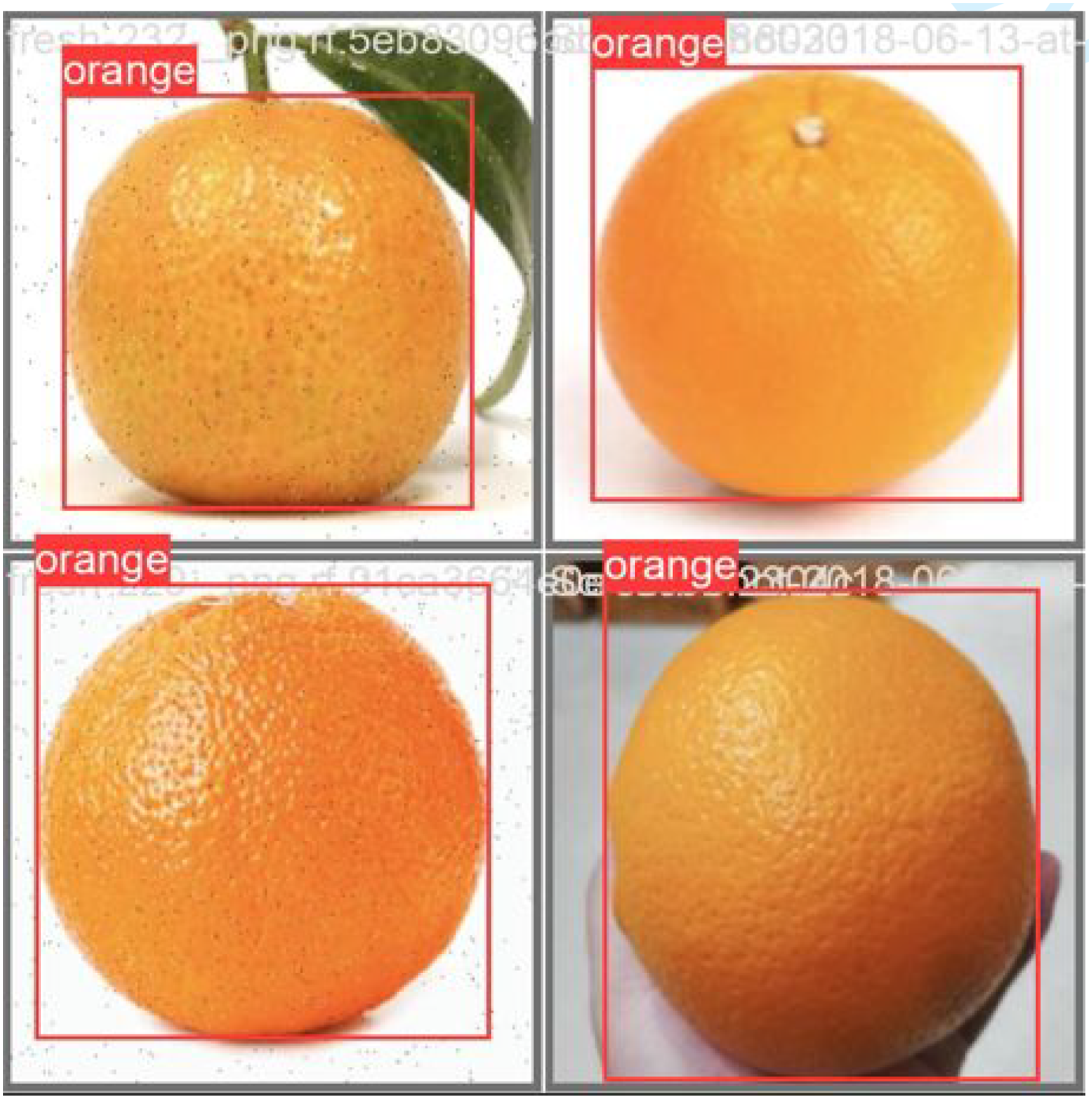
Examples of good quality oranges.

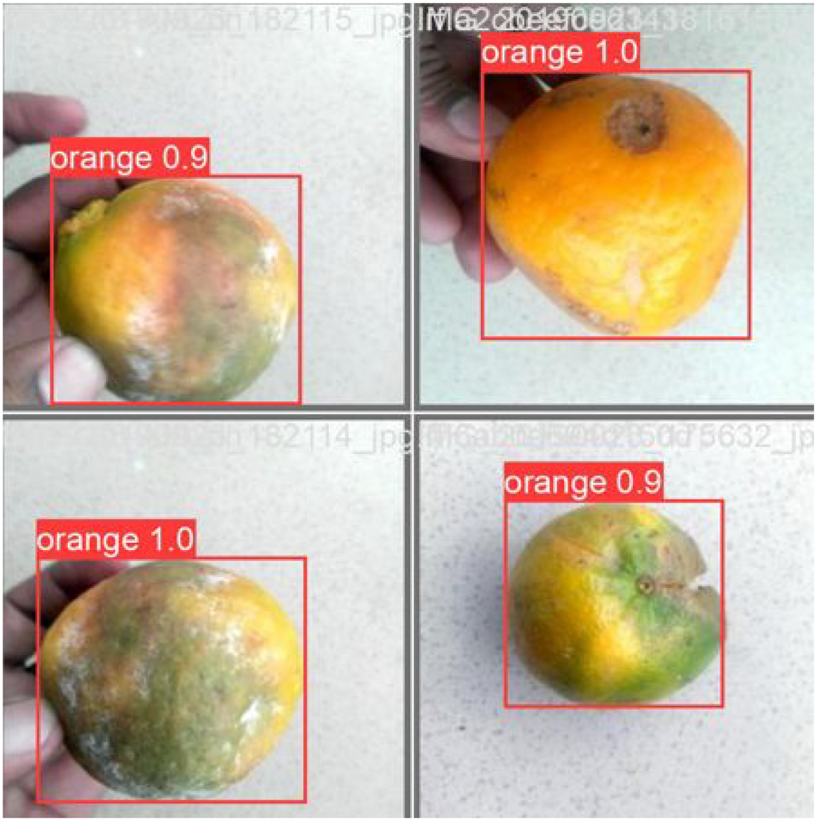
On the other hand, poor quality oranges often exhibit faded or uneven color, with blotchy spots indicating uneven ripening or disease. The shape of these oranges may have dents, distortions, or deformations, as shown in Figure 5, suggesting that the orange has experienced significant impact or has grown under unfavorable conditions. The skin of poor quality oranges is typically rough, with bruises, scars, or signs of damage, indicating that the orange has been damaged or improperly stored, affecting its internal quality.

Figure 5.

Examples of poor quality oranges.

In addition to the primary criteria, there are supplementary factors that help provide a more comprehensive evaluation of orange quality. Good oranges are typically uniform in size and match the average size for their variety, as shown in Figure 6. The weight of the orange is also an important factor; it should feel heavy for its size, indicating juiciness and good flavor. A natural and pleasant aroma is another sign of high quality. Finally, when gently pressed, a good orange should have slight elasticity without deep indentation, indicating freshness and that the orange is not spoiled. These criteria ensure that the selected oranges are not only tasty but also safe and nutritious, meeting quality standards for production and consumption.

Figure 6.

Examples of damaged oranges.

Results and discussions

Orange classification model

The model for classifying good and bad oranges is built on a DCNN using the MobileNetV2 architecture. DCNNs are a prominent type of deep learning model with the capability to learn and extract features from images, enabling accurate object classification. MobileNetV2, a lightweight and efficient DCNN architecture, is particularly suitable for mobile and embedded applications and was chosen as the foundation for this model. ➢

Backbone network: The backbone network is the core part of the model used to extract features from the input images. MobileNetV2, designed by Google, has several outstanding features:

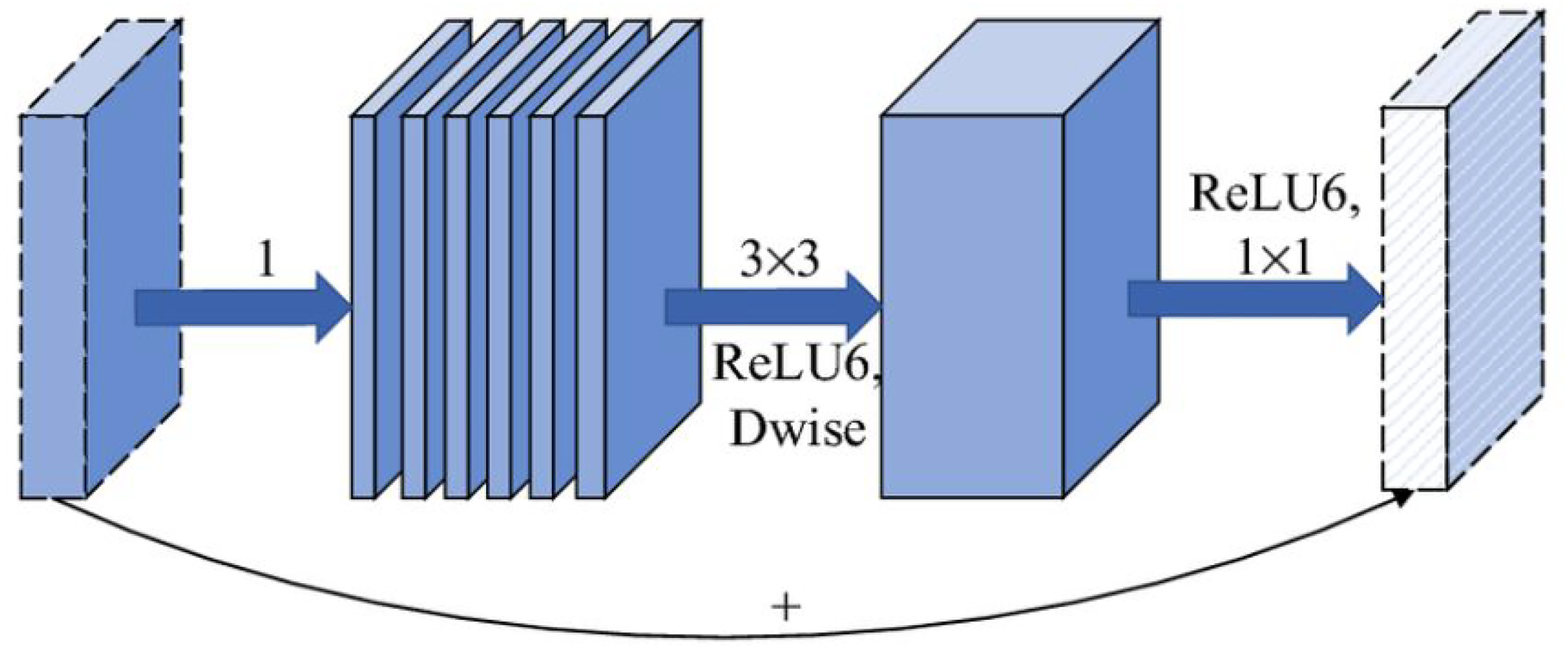
✓ Depthwise separable convolutions:^52,53 Instead of using standard convolution layers, MobileNetV2 applies depthwise separable convolutions to minimize the number of parameters and computations while maintaining high performance as shown in Figure 7. This technique separates the application of spatial filters and depthwise filters into two distinct steps.^54,55 First, a depthwise convolution layer is applied to each channel individually, and then, a pointwise convolution (1 × 1 convolution) combines the results. This method allows the model to process images more efficiently and extract important features such as color, texture, and shape of the oranges.^56–58

✓ Linear bottlenecks: The bottleneck layers in MobileNetV2 use linear activations after performing 1 × 1 convolutions as in Figure 8.^59,60 This helps minimize the loss of important information caused by nonlinear activation functions, especially in low-dimensional feature spaces. These bottleneck layers work by first expanding the feature space with an expansion convolution layer, then applying spatial transformations, and finally compressing back to the original size.^61,62 This technique allows the model to retain important features related to the quality of oranges, such as shine and uniform color.

✓ Inverted residuals: The inverted residual block architecture in MobileNetV2 reverses the logic of traditional residual blocks as Figure 9. In traditional residual blocks,^63,64 the input is compressed before applying complex transformations and then expanded again. In inverted residual blocks, the input is first expanded before applying transformations and then compressed again. This enhances feature extraction capability while keeping the number of parameters and computations low. Inverted residual blocks allow the model to learn more complex features, such as minor defects or blemishes on the orange surface.

➢

Detection branch: The detection branch is the final part of the model, where the features extracted by the backbone network are used for classification. In this model, the features from MobileNetV2 are used directly without fine-tuning to leverage the prelearned features from the base network. The detection branch utilizes these features to identify and classify objects in the images based on the extracted characteristics.

➢

Classification layer: After feature extraction, the features are passed through a classification layer as shown in Figure 10. This layer has two outputs, corresponding to the two classes of good and bad oranges. The features extracted from the images are used to determine whether an orange is good or bad based on factors such as color, shine, and the presence of defects on the surface. The classification layer uses a softmax function to provide the probability for each class, thereby making the final decision about the quality of the orange.

Figure 7.

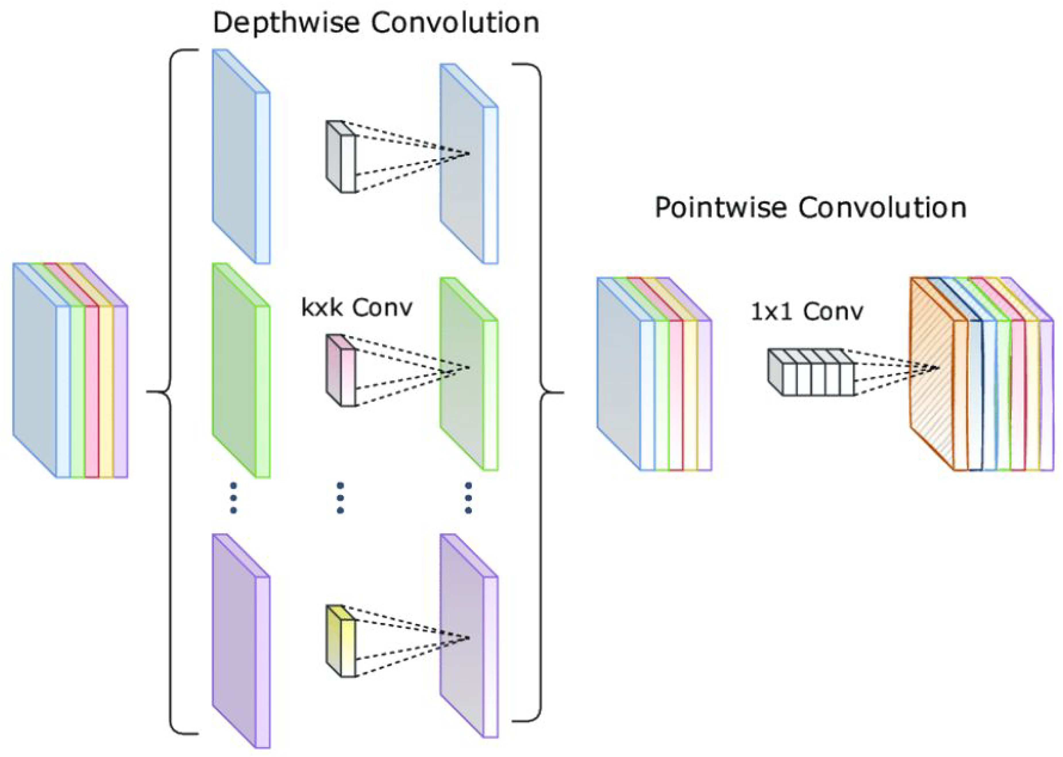
Depthwise separable convolutions model.

Figure 8.

Linear bottlenecks model.

Figure 9.

Inverted residuals model.

Figure 10.

Layers used in the model.

This classification model employs advanced techniques in CNNs to extract important features from orange images and classify them into two categories: good and bad oranges. The combination of efficient convolution layers and a robust classification layer enables the model to achieve high accuracy in classifying the quality of oranges. Techniques like depthwise separable convolutions, linear bottlenecks, and inverted residuals not only help the model process data efficiently but also maintain high performance with minimal parameters and computations. This is particularly important in mobile and embedded applications, where computational resources and memory are often limited.

Orange detection model

Proposed technology in the study

In this study, the paper proposes a combination of two models: DCNN and feature pyramid network (FPN). ➢

DCNN: DCNN is the primary technology used in this model to extract features from the input images as shown in Figure 11. DCNN is a specialized type of neural network, particularly effective in tasks related to image processing and object recognition. The convolutional layers in DCNN are efficiently arranged to learn features at various levels of detail. Initially, the first layers in the network learn basic features such as edges, corners, and textures. As the network goes deeper, the subsequent layers learn more complex features such as shapes and structures of objects in the images.

➢

FPN: FPN is a network structure used to detect objects of various sizes as shown in Figure 12. FPN combines features at different levels of the CNN, creating a multiscale representation of the features. Specifically, FPN uses features from different layers within the CNN and combines them to produce higher resolution features. This allows the model to effectively detect both large and small objects in images. FPN operates by creating a feature pyramid from the features extracted at different layers of the CNN. The top layers of the pyramid represent detailed features with high resolution, aiding in the detection of small objects. The bottom layers of the pyramid represent more general features with low resolution, helping to detect large objects. By combining features from multiple layers, FPN improves the model's accuracy and performance in detecting objects of various sizes and scales.

Figure 11.

Proposed DCNNs in this study.

Figure 12.

Proposed FPN in this study.

The model for classifying and detecting good and bad oranges utilizes advanced technologies like CNN and FPN to extract and combine features from input images. CNN helps learn features at various levels of detail, while FPN allows for effective detection of objects at different sizes. The combination of these two technologies ensures that the model can recognize and classify oranges with high accuracy, regardless of the size and scale of the oranges in the images.

Performance evaluation of the detection model

The performance of the orange detection model was evaluated based on precision, recall, and the analysis of misclassification cases, as depicted in Figure 13. ➢

Orange detection accuracy: The model demonstrated strong performance by correctly identifying 88 orange samples. The precision for the “orange” class was 95.7%, meaning that out of all predicted oranges, 95.7% were correctly classified. This indicates that the model is highly effective in identifying oranges from the test dataset.

➢

Background misclassification: However, there were some challenges in differentiating between oranges and the background. The model misclassified four background samples as oranges, resulting in some confusion. Despite this, the recall for the “orange” class was 94.6%, meaning that the model correctly identified 94.6% of all actual orange samples. While this recall value is high, there is room for improvement in distinguishing between oranges and the background.

➢

Areas for improvement: Additionally, the model incorrectly classified five orange samples as background, suggesting that it struggles with certain background features that resemble orange characteristics. These misclassifications could be attributed to image quality or similarities in the visual features of the oranges and background.

Figure 13.

Confusion matrix showing the model's misclassifications.

In summary, the model performed well with high precision (95.7%) and recall (94.6%) in detecting oranges. However, it requires further refinement to reduce the number of misclassifications between oranges and the background. Enhancements could be made by fine-tuning the model, diversifying the training data, and applying more advanced feature extraction techniques. With these improvements, the model could achieve even higher accuracy and better distinguish between oranges and background elements.

Training process and performance evaluation

During training, the model exhibited significant improvements in loss metrics and performance indicators, reflecting the model's increasing accuracy and efficiency. The bounding box loss steadily decreased from 0.7 to 0.2, indicating better localization of objects over successive epochs. Similarly, the classification loss dropped from 1.5 to 0.25, showing rapid improvement during the initial epochs, followed by fine-tuning. The distribution focal loss also decreased from 1.4 to 1.0, signaling improved accuracy in predicting object positions (see Figure 14).

Figure 14.

Graph represents showing precision/loss curves during training and top-level testing.

Regarding performance metrics, precision initially started high, dipped slightly in the early epochs, and then stabilized between 0.8 and 0.9, likely due to learning rate adjustments. Once stabilized, this indicated reliable classification accuracy. Recall began at a lower value, improved significantly during the early epochs, and stabilized around 0.9, suggesting that the model became better at detecting objects over time.

Overall, the training process demonstrated positive trends, with consistent reductions in loss values and improved stability in key performance metrics. These results indicate that the model is learning effectively and achieving high performance in object classification and detection. Moving forward, the next steps should focus on fine-tuning the training parameters and addressing misclassifications between oranges and the background to further enhance performance.

Testing process and performance evaluation

During the testing phase, the model's loss and performance metrics showed a clear improving trend, despite some initial fluctuations. The bounding box loss (val/box_loss) fluctuated initially but decreased from around 4 to 0, indicating improved accuracy in object localization. These fluctuations were likely due to the complexity of the test set or instability early in training. The classification loss (val/cls_loss) also trended downward, with occasional fluctuations, suggesting an overall enhancement in the model's classification ability, though some variability might have been caused by overfitting or test set variability. Similarly, the distribution focal loss (val/dfl_loss) decreased from 1.4 to 1.0, reflecting the model's increasing accuracy in predicting object positions (see Figure 15).

Figure 15.

Graph represents showing precision/loss curves during training and bottom-level testing.

In terms of performance metrics, mean average precision (mAP) at IoU = 0.50 (metrics/mAP50(B)) started low, improved significantly, and stabilized around 0.9, indicating the model's growing effectiveness in object detection. Mean average precision at IoU thresholds from 0.50 to 0.95 (metrics/mAP50-95(B)) also improved, stabilizing between 0.8 and 0.9, providing a more comprehensive evaluation of the model's performance across various overlap thresholds.

The overall trend of both loss values and performance metrics indicates consistent improvement during both training and testing phases, suggesting effective ongoing learning. Although the initial fluctuations in testing metrics are normal, the decreasing loss and increasing accuracy metrics confirm that the model is learning efficiently and not overfitting.

Compare and test the model

Model present

The proposed model achieved an overall accuracy of 99.53%, not 100% as previously mentioned. This correction ensures consistency with the results observed in the confusion matrix, where minor misclassifications were noted. In addition to accuracy, we report the following key performance metrics to provide a more comprehensive evaluation of the model's classification ability:

Precision: The model achieved a precision of 99% for the “orange_good” class and 100% for the “orange_bad” class, demonstrating its strong ability to correctly identify “bad” oranges without incorrectly classifying “good” ones.

Recall: The recall for the “orange_good” class was 100%, meaning all good oranges were correctly identified, and 99% for the “orange_bad” class, indicating that only a small number of bad oranges were missed.

F1-score: The F1-score, which balances precision and recall, was 0.99 for “orange_good” and 1.00 for “orange_bad,” reflecting the strong overall performance of the model.

This thorough evaluation highlights the reliability of the model in classifying oranges, providing both high precision and recall while addressing the minor misclassifications observed. The present model is used to classify oranges into two categories: “orange_good” and “orange_bad.” The recognition results are presented in the table below, detailing specific evaluation metrics when operating on image data as Table 2.

➢

Precision is the accuracy of positive predictions compared to the total number of positive predictions. For the “orange_good” class, precision is 0.99, meaning that 99% of the oranges predicted to be good are correct. For the “orange_bad” class, precision is 1.00, meaning that all oranges predicted to be bad are indeed bad. This indicates that the model rarely misclassifies bad oranges as good, ensuring high reliability in identifying bad oranges as shown in Figure 16.

➢

Recall is the accuracy of positive predictions compared to the total number of actual positive samples. For the “orange_good” class, recall is 1.00, meaning that the model correctly identifies all good oranges, ensuring that no good oranges are missed. For the “orange_bad” class, recall is 0.99, meaning the model correctly identifies 99% of the bad oranges, missing only a very small number of bad oranges as in Figure 17. This result shows that the model is very effective in identifying good oranges while only missing a small percentage of bad ones.

➢

F1-score is the harmonic mean of precision and recall, providing a balanced measure between these two metrics. The F1-score for the “orange_good” class is 0.99, indicating that the model maintains a good balance between precision and recall for good oranges. For the “orange_bad” class, the F1-score is 1.00, indicating a perfect balance between precision and recall for bad oranges. This demonstrates that the model has very robust and stable classification capabilities for both classes.

➢

The overall accuracy of the model is 1.00 out of 637 test samples. This means that all samples were correctly predicted, with no misclassifications. This level of accuracy indicates that the model has outstanding and reliable performance in classifying the quality of oranges.

➢

Macro average and weighted average are unweighted and weighted averages of precision, recall, and F1-score. Macro average provides an overall view of the model's performance without being influenced by class sample size differences, achieving 0.99 for precision and 1.00 for recall and F1-score. This shows that the model performs very well across both classes. Weighted average, which calculates the average based on the number of samples in each class, also reaches the highest level (1.00) for all metrics, confirming that the model operates stably and effectively across the entire dataset, including classes with larger sample sizes.

Figure 16.

Precision confidence curve of the present model.

Figure 17.

Precision recall curve of the present model.

Table 2.

Performance of the proposed model.

	Precision	Recall	F1-score	Support
0 orange_good	0.99	1.00	0.99	292
1 orange_bad	1.00	0.99	1.00	345
accuracy	\|\|	\|\|	1.00	637
macro_avg	0.99	1.00	1.00	637
weighted_avg	1.00	1.00	1.00	637

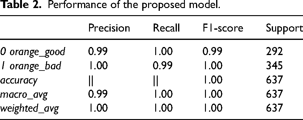
The present model delivers excellent results in classifying oranges based on image data, with near-perfect accuracy and other metrics. High precision and recall for both “orange_good” and “orange_bad” classes indicate that the model not only correctly identifies good oranges but also rarely misclassifies bad oranges as good. The overall accuracy of 1.00, along with the maximum macro and weighted averages, shows that the model operates stably and effectively across the entire dataset. This demonstrates the present model's significant potential for practical application, enhancing efficiency and accuracy in the quality control process of oranges. Achieving such high evaluation metrics attests to the capability and performance of the present model in the field of agricultural product classification.

Random Kaggle model

This random model was trained based on the fruits dataset and used the ResNet50V2 architecture to classify oranges into two categories: “freshoranges” and “rottenoranges.” The evaluation results are presented in the table below, detailing specific model evaluation metrics in Table 3. ➢

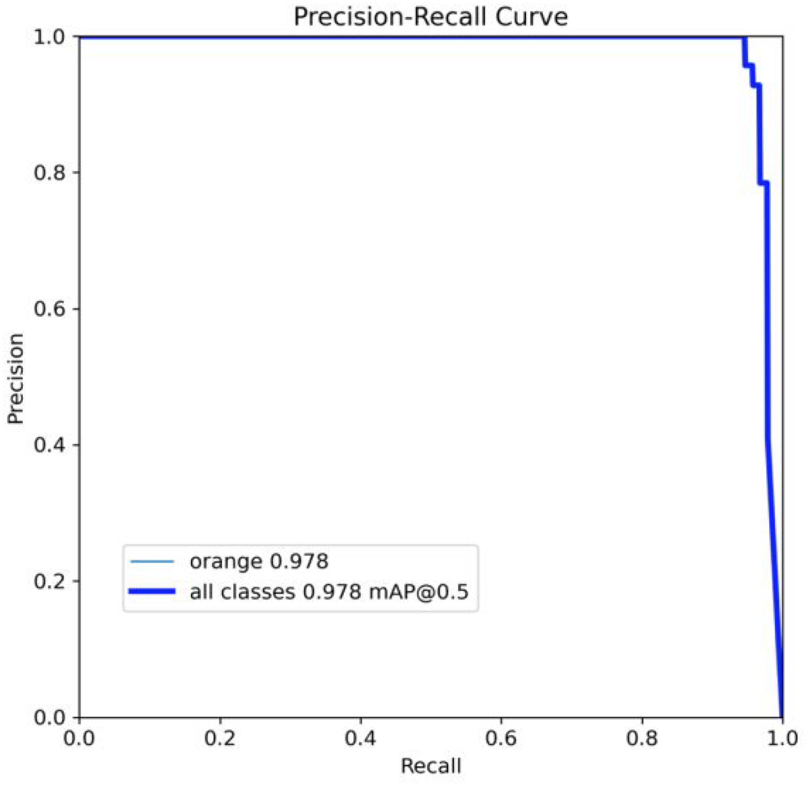
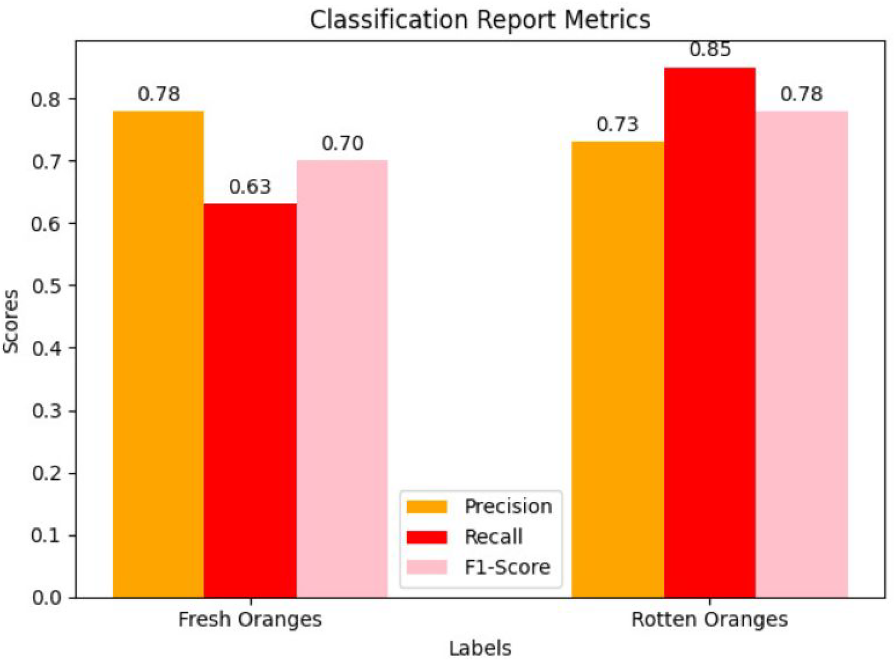
Precision is the accuracy of positive predictions compared to the total number of positive predictions. For the “freshoranges” class, precision is 0.78, meaning that 78% of the oranges predicted to be fresh are actually fresh. For the “rottenoranges” class, precision is 0.73, meaning that 73% of the oranges predicted to be rotten are indeed rotten as in Figure 18. This indicates that the model has a fairly good capability of identifying both fresh and rotten oranges, but there are still quite a few incorrect predictions.

➢

Recall is the accuracy of positive predictions compared to the total number of actual positive samples. For the “freshoranges” class, recall is 0.63, meaning that the model correctly identifies 63% of the fresh oranges. For the “rottenoranges” class, recall is 0.85, meaning the model correctly identifies 85% of the rotten oranges as shown in Figure 19. This result shows that the model is more effective in identifying rotten oranges compared to fresh ones.

➢

F1-score is the harmonic mean of precision and recall. The F1-score for the “freshoranges” class is 0.70, indicating that the model maintains a fairly good balance between precision and recall for fresh oranges. For the “rottenoranges” class, the F1-score is 0.78, showing a better balance between precision and recall for rotten oranges in Figure 20.

➢

The overall accuracy of the model is 0.75 out of 637 test samples. This means that the model correctly classified 75% of the total orange samples, indicating that the model performs quite well but still has room for improvement.

➢

Macro average and weighted average for precision, recall, and F1-score show that the model performs stably and relatively well across all data classes. Macro average provides an overall view of the model's performance without being influenced by class sample size differences. Weighted average, which calculates the average weighted by the number of samples in each class, confirms that the model operates stably and effectively across the entire dataset.

Figure 18.

Precision confidence curve of random Kaggle model.

Figure 19.

Recall confidence curve of the random Kaggle model.

Figure 20.

F1-score confidence curve of random Kaggle model.

Table 3.

Performance of the random Kaggle model.

	Precision	Recall	F1-score	Support
freshoranges	0.78	0.63	0.70	292
rottenoranges	0.73	0.85	0.78	345
accuracy	\|\|	\|\|	0.75	637
macro_avg	0.75	0.74	0.74	637
weighted_avg	0.75	0.75	0.74	637

The random classification model achieves acceptable results in classifying oranges, with an overall accuracy of 0.75. Precision and recall for both “freshoranges” and “rottenoranges” show that the model is better at identifying and classifying rotten oranges than fresh ones. The F1-score indicates a fairly good balance between precision and recall, but there is still room for improvement to enhance performance. Macro average and weighted average confirm that the model operates stably across all data classes. However, to improve performance, especially in identifying fresh oranges, the model needs further tuning and improvement.

Comparison between the present model and the random model

The confusion matrix of the present model shows high classification performance as shown in Figure 21. Out of the total test samples, 292 “orange_good” samples and 342 “orange_bad” samples were correctly classified. Only three “orange_bad” samples were misclassified as “orange_good,” and no “orange_good” samples were misclassified. This indicates that the present model has high accuracy, with a clear ability to distinguish between good and bad oranges as shown in Figure 22. The present model demonstrates high sensitivity and specificity, showing its ability to accurately classify without missing important samples or making incorrect classifications.

Figure 21.

The confusion matrix of the present model.

Figure 22.

Accuracy of cam quality of the recognition present model.

Conversely, the confusion matrix of the random model from Kaggle shows lower classification performance as shown in Figure 23. Specifically, 184 “freshoranges” samples and 292 “rottenoranges” samples were correctly classified. However, 108 “freshoranges” samples were misclassified as “rottenoranges,” and 53 “rottenoranges” samples were misclassified as “freshoranges.” This significant misclassification indicates that the random model does not clearly distinguish between different types of oranges, leading to many errors in classification as shown in Figure 24.

Figure 23.

The confusion matrix of the random Kaggle model.

Figure 24.

Accuracy of cam quality of the recognition random Kaggle model.

After comparison, the results show that the present model significantly outperforms the random model from Kaggle in classifying oranges. The present model achieved an overall accuracy of 100%, with near-perfect precision, recall, and F1-score for both “orange_good” and “orange_bad” classes. In contrast, the random model only achieved an accuracy of 75% and had many misclassifications, especially between “freshoranges” and “rottenoranges.”

An important factor contributing to the superior performance of the present model is the use of augmented data with techniques such as flipping images, hue transformation, brightness adjustment, and noise addition. The test data was also augmented similarly, helping the present model learn many features and become more robust. In contrast, the random model from Kaggle used raw data without augmentation, leading to poorer learning and classification capabilities. This confirms that the present model has higher performance and reliability, making it more suitable for practical applications, especially in quality control processes for oranges. The superiority of the present model in handling data and accurately classifying underscores its high capability and performance in the field of agricultural product classification.

To provide a comprehensive comparison of our proposed MobileNetV2 model, we tested several other state-of-the-art CNN architectures, including ResNet50, VGG16, and InceptionV3, using the same dataset and evaluation metrics The performance metrics for each model are summarized in Table 4, with a detailed breakdown of accuracy, precision, recall, and F1-score.

Table 4.

The comparison of our proposed MobileNetV2 model.

Model	Accuracy (%)	Precision (%)	Recall (%)	F1-score (%)
MobileNetV2	95.3	95.7	94.6	95.1
ResNet50	93.1	92.5	91.3	91.9
VGG16	92.0	91.8	90.1	90.9
InceptionV3	94.2	93.9	93.2	93.5

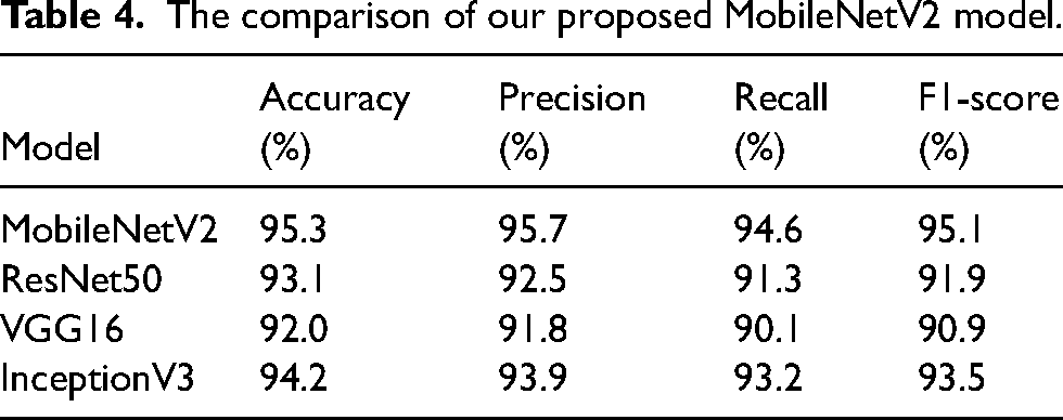
From the results, the MobileNetV2 model outperforms the other architectures in terms of precision and F1-score, indicating that it is better at minimizing false positives while maintaining a strong balance between precision and recall. The ResNet50 and InceptionV3 models performed competitively, with InceptionV3 showing slightly higher recall but lower precision. VGG16, while robust, exhibited lower overall accuracy and precision compared to the other models. This comparison confirms that MobileNetV2 is particularly effective for the orange classification task, likely due to its lightweight architecture and efficient feature extraction. The comparison also highlights the benefits of using data augmentation and fine-tuning strategies, which were applied across all models to ensure a fair evaluation.

To comprehensively evaluate the proposed MobileNetV2 model, we compared our results with several other studies in the field of fruit and agricultural product classification using deep neural network architectures. Table 5 presents a comparison of accuracy, mAP, and other performance metrics from previously published studies.

Table 5.

The comparison of accuracy, mAP, and other performance metrics.

Study	Model used	Accuracy (%)	mAP	F1-score (%)
This study (MobileNetV2)	MobileNetV2 + augmentation	95.3	0.90	95.1
^33,50	ResNet50	92.7	0.87	91.5
⁶⁵	InceptionV3	94.2	0.88	93.3
⁶⁶	VGG16	90.5	0.85	90.1

The results show that the MobileNetV2 model in our study achieved higher accuracy and F1-score compared to studies using other architectures, such as ResNet50 and InceptionV3. Although these models performed relatively well, the use of data augmentation and hyperparameter optimization contributed to the superior performance of MobileNetV2, especially in terms of the F1-score, which reflects the balance between precision and recall. Additionally, the mAP of our MobileNetV2 model was higher than in other studies, indicating the model's effectiveness in accurately detecting and classifying orange samples in the test dataset. These findings demonstrate that using MobileNetV2 with appropriate optimization techniques provides an effective solution for real-world agricultural classification tasks.

Conclusion and future directions

This study successfully introduced and implemented a DCNN model based on the MobileNetV2 architecture to classify the quality of oranges. Advanced techniques such as depthwise separable convolutions, linear bottlenecks, and inverted residuals were applied to optimize performance and reduce the computational load of the model. Additionally, the use of data augmentation methods such as image flipping, grayscale transformation, hue adjustment, brightness adjustment, and noise addition helped the model learn and generalize better. The present model achieved outstanding performance with an overall accuracy of 99.53%∼100% with nearly perfect precision, recall of 95.7%, and F1-score of 94.6% for both “orange_good” and “orange_bad” classes, along with nearly perfect precision, recall, and F1-score for both “orange_good” and “orange_bad” classes. These results demonstrate the model's excellent classification capability, particularly in clearly distinguishing between good and bad oranges. The confusion matrix also confirms the model's high sensitivity and specificity, with only a very few misclassifications.

This research opens up several potential development directions to further enhance the model's performance and practical applications. First, expanding the dataset with larger and more diverse datasets from various sources can increase the model's representativeness and generalization ability. Second, applying additional advanced data augmentation techniques such as random cropping, zooming, rotation, and contrast adjustment can strengthen the model's robustness under different conditions. Third, fine-tuning the model's hyperparameters can help identify the optimal configuration, thereby improving performance and accuracy. Fourth, combining multiple models to create a more powerful ensemble model can enhance classification accuracy and reliability. Fifth, the model is deployed on mobile and embedded devices to test its functionality in real-world environments, including quality control processes at agricultural processing facilities. Finally, the research is extended to other types of agricultural products to evaluate the model's versatility and effectiveness in general agricultural product classification and quality control.

In summary, this study demonstrated the capability and efficiency of the MobileNetV2-based DCNN model in classifying orange quality. With the achieved results, the research opens up numerous potential development directions to further improve and expand the model's applications, not only in the agricultural sector but also in various other fields of computer vision and deep learning.

Footnotes

Author contributions

Phan Thi Huong: conceptualization, software, and writing—review and editing. Lam Thanh Hien: formal analysis and investigation. Nguyen Minh Son: conceptualization, methodology, and writing—review and editing. Huynh Cao Tuan: investigation, formal analysis, and visualization. Thanh Q. Nguyen: supervision, writing—review and editing, and visualization.

Data availability

The authors confirm that the data supporting the findings of this study are available within the article and its supplementary materials.

Declaration of conflicting interests

This is to certify that to the best of authors' knowledge, the content of this manuscript is original. The paper has not been submitted elsewhere nor has been published anywhere. Authors confirm that the intellectual content of this paper is the original product of our work and all the assistance or funds from other sources have been acknowledged.

Ethical approval and informed consent

Data usage should not cause harm to individuals or communities. Clear and open communication regarding data collection, storage, and usage practices is essential to establish trust and accountability.

Funding

This research was conducted without any financial support from funding agencies. No grants were received from governmental, private, or non-profit organizations for the execution of this study.

ORCID iD

Thanh Q. Nguyen

References

Gomaa

Zain elabdeen

Elnashar

, et al. Brain tumor X-ray images enhancement and classification using anisotropic diffusion filter and transfer learning models. Int J Inf Technol 2024; 16: 3771–3779. https://doi.org/10.1007/s41870-024-01830-0

Mohammadi

. Brain tumor diagnosis from MRI based on Mobilenetv2 optimized by contracted fox optimization algorithm. Heliyon 2023; 10: e23866.

Peng

Zhao

, et al. Recognition of tomato leaf diseases based on DIMPCNET. Agronomy 2023; 13: 1812.

Gulzar

Ünal

Aktaş

, et al. Harnessing the power of transfer learning in sunflower disease detection: a comparative study. Agriculture 2023; 13: 1479.

Salem

Hassan

Hamdy

. Impact of transfer learning compared to convolutional neural networks on fruit detection. J Intell Fuzzy Syst 2024; 46: 7791–7803.

Suhendar

Efelina

Ziveria

. Fruit quality classification using convolutional neural network. J Phys Conf Ser 2022; 2377: 012015.

Yang

Wang

Nie

, et al. A lightweight YOLOv8 tomato detection algorithm combining feature enhancement and attention. Agronomy 2023; 13: 1824.

Shahi

Sitaula

Neupane

, et al. Fruit classification using attention-based MobileNetV2 for industrial applications. PLoS One 2022; 17: e0264586.

Ananthanarayana

Ptucha

Kelly

. Deep learning based fruit freshness classification and detection with CMOS image sensors and edge processors. Electr Imag 2020; 32: 1–7.

10.

Lamba

Kukreja

Rashid

, et al. A novel fine-tuned deep-learning-based multi-class classifier for severity of paddy leaf diseases. Front Plant Sci 2023; 14: 1234067.

11.

Mohannad Alkanan

aYG

. Enhanced corn seed disease classification: leveraging MobileNetV2 with feature augmentation and transfer learning. Front Appl Math Stat 2024; 9: 1320177.

12.

Metlek

Çetıner

. ResUNet+: a new convolutional and attention block-based approach for brain tumor segmentation. IEEE Access 2023; 11: 69884–69902.

13.

Chincholkar

Srivastava

Pawanarkar

, et al. Deep learning techniques in liver segmentation: evaluating U-Net, Attention U-Net, ResNet50, and ResUNet models. In: 14th IEEE International Conference on Cloud Computing, Data Science & Engineering (Confluence), Noida, India, 18–19 January 2024, pp. 775–779.

14.

Alkanan

Gulzar

. Enhanced corn seed disease classification: leveraging MobileNetV2 with feature augmentation and transfer learning. Front Appl Math Stat 2024; 9: 1320177.

15.

Gulzar

. Fruit image classification model based on MobileNetV2 with deep transfer learning technique. Sustainability 2023; 15: 1906.

16.

Chincholkar

Srivastava

Pawanarkar

, et al. Deep learning techniques in liver segmentation: evaluating U-Net, Attention U-Net, ResNet50, and ResUNet models. In: 4th IEEE International Conference on Cloud Computing, Data Science & Engineering (Confluence), pp.775–779, 2024.

17.

Sowrirajan

Srinivasan

Kalluri

, et al. Improved brain tumor segmentation using UNet-LSTM architecture. SN Computer Science 2024; 5: 496.

18.

Zhao

. Potato leaf disease segmentation method based on improved UNet. Appl Sci 2023; 13: 11179.

19.

Ramya

Lenin Marksia

Valli Suseela

, et al. Advancing brain lesion classification in CT images: a transfer learning approach with convolutional neural networks. In: 3rd IEEE International Conference on Innovative Mechanisms for Industry Applications (ICIMIA), pp. 1112–1118, 2023.

20.

Arif Budiman

Suharyat

Yulianti

. Effectiveness of using CT scan in EarlyDetection of brain tumor. Indones J Eng Educ Technol 2024; 2: 164–172.

21.

Liu

Zhu

, et al. Transsea: hybrid CNN–transformer with semantic awareness for 3-D brain tumor segmentation. IEEE Trans Instrum Meas 2024; 73: 16–31.

22.

Telkar

Anusudha

. Advances and challenges in brain tumor classification and segmentation: a comprehensive review. In: IEEE International Conference on Inventive Computation Technologies (ICICT), pp. 860–865, 2024.

23.

Karim

Tong

, et al. Developments in brain tumor segmentation using MRI: deep learning insights and future perspectives. IEEE Access 2024; 12: 26875–26896.

24.

Çetiner

. Citrus disease detection and classification using based on convolution deep neural network. Microprocess Microsyst 2022; 95: 104687.

25.

Ortiz

DJN

Lopez

SAM

. Automatic identification of banana quality with Deep Neural Network Classification (DNN). Cien Tecnol 2022; 1: 37–56.

26.

Azeem

Javaid

Khalil

, et al. Neural networks for the detection of COVID-19 and other diseases: prospects and challenges. Bioengineering 2023; 10: 850.

27.

Bhuvaneswari Thomas

Nithish

, et al. Brain tumor diagnosis using deep learning: a literature review. In: Second IEEE International Conference on Emerging Trends in Information Technology and Engineering (ICETITE), pp. 1–8, 2024.

28.

Das

Mohapatra

Pattanaik

, et al. Target driven autoencoder: a supervised learning approach for tumor segmentation. In: IEEE International Conference on Emerging Systems and Intelligent Computing (ESIC), pp. 273–277, 2024.

29.

Karim

Tong

, et al. Developments in brain tumor segmentation using MRI: deep learning insights and future perspectives. IEEE Access 2024; 12: 26875–26896.

30.

Pinheiro

Moreira

Queirós da Silva

, et al. Deep learning YOLO-based solution for grape bunch detection and assessment of biophysical lesions. Agronomy 2023; 13: 1120.

31.

Singh

Shivam Kumar

. Orange fruit recognition using neural networks. In: Proceedings of the international conference on computational intelligence and sustainable technologies: ICoCIST 2021. Singapore: Springer Nature Singapore, 2022, pp.417–427.

32.

Chakraborty

Javed Mehedi Shamrat

Billah

, et al. Implementation of deep learning methods to identify rotten fruits. In: 2021 IEEE 5th International Conference on Trends in Electronics and Informatics (ICOEI), pp. 1207–1212, 2021.

33.

Singh

Gupta

Kumar

. Fresh and rotten fruit detection using deep CNN and MobileNetV2. In: International conference on advances in IoT and security with AI. Singapore: Springer Nature Singapore, 2023, pp.219–231.

34.

Rehman

MZU

Ahmed

Khan

, et al. Classification of citrus plant diseases using deep transfer learning. Comput Mater Contin 2021; 70: 1401–1417.

35.

Kumar

Pandey

Raghav

, et al. A deep learning approach for multiclass orange disease classification. In: 2024 IEEE 2nd International Conference on Disruptive Technologies (ICDT), pp. 184–189, 2024.

36.

Kerta

Rangkuti

Tantio

. Comparison of deep convolutional neural network architectures for fruit categorization. Int J Electr Comput Eng Syst 2024; 15: 247–259.

37.

Gulzar

. Fruit image classification model based on MobileNetV2 with deep transfer learning technique. Sustainability 2023; 15: 1906.

38.

Gulzar

. Enhancing soybean classification with modified inception model: a transfer learning approach. Emir J Food Agric 2024; 36: 1–9.

39.

Alkanan

Gulzar

. Enhanced corn seed disease classification: leveraging MobileNetV2 with feature augmentation and transfer learning. Front Appl Math Stat 2024; 9: 1320177.

40.

Liu

Shi

, et al. Towards better analysis of deep convolutional neural networks. IEEE Trans Vis Comput Graph 2016; 23: 91–100.

41.

Tustison

Avants

Gee

. Learning image-based spatial transformations via convolutional neural networks: a review. Magn Reson Imaging 2019; 64: 142–153.

42.

Patel

. A comprehensive study of applying convolutional neural network for computer vision. Int J Adv Sci Technol 2020; 6: 2161–2174.

43.

Ayeni

. Convolutional neural network (CNN): the architecture and applications. Appl J Phys Sci 2022; 4: 42–50.

44.

Sarıgül

Ozyildirim

Avci

. Differential convolutional neural network. Neural Netw 2019; 116: 279–287.

45.

Jogin

Madhulika

Divya

, et al. Feature extraction using convolution neural networks (CNN) and deep learning. In: 2018 IEEE 3rd IEEE International Conference on Recent Trends in Electronics, Information & Communication Technology (RTEICT), pp. 2319–2323, 2018.

46.

Patel

. A comprehensive analysis of convolutional neural network models. Int J Adv Sci Technol 2020; 29: 771–777.

47.

Seymen

Ölmez

Doğan

, et al. Customer churn prediction using ordinary artificial neural network and convolutional neural network algorithms: a comparative performance assessment. Gazi Univ J Sci 2023; 36(2): 720–733.

48.

Huang

Xiong

Chen

, et al. Slope stability prediction based on a long short-term memory neural network: comparisons with convolutional neural networks, support vector machines and random forest models. Int J Coal Sci Technol 2023; 10: 18.

49.

Jiang

Wang

Liu

. Comparisons of convolutional neural network and other machine learning methods in landslide susceptibility assessment: a case study in Pingwu. Remote Sens (Basel) 2023; 15: 798.

50.

Ahad

Song

, et al. Comparison of CNN-based deep learning architectures for rice diseases classification. Artif Intell Agric 2023; 9: 22–35.

51.

Naskath

Sivakamasundari

Alif Siddiqua Begum

. A study on different deep learning algorithms used in deep neural nets: MLP SOM and DBN. Wirel Pers Commun 2023; 128: 2913–2936.

52.

Gao

Qian

. Exponential linear units-guided depthwise separable convolution network with cross attention mechanism for hyperspectral image classification. Sign Process 2023; 210: 108995.

53.

Batool

Byun

Y-C

. Lightweight EfficientNetB3 model based on depthwise separable convolutions for enhancing classification of leukemia white blood cell images. IEEE Access 2023; 1: 37203–37215.

54.

Tseng

F-H

Yeh

K-H

Kao

F-Y

, et al. MiniNet: dense squeeze with depthwise separable convolutions for image classification in resource-constrained autonomous systems. ISA Trans 2023; 123: 120–130.

55.

Tian

. Hybrid convolutional network combining multiscale 3D depthwise separable convolution and CBAM residual dilated convolution for hyperspectral image classification. Remote Sens (Basel) 2023; 15: 4796.

56.

Wang

Shao

, et al. A lightweight distillation CNN-transformer architecture for remote sensing image super-resolution. Int J Dig Earth 2023; 16: 3560–3579.

57.

Wang

Cheikh

. Discriminating spectral–spatial feature extraction for hyperspectral image classification: a review. Sensors 2024; 24: 2987.

58.

Zhao

Zhang

Xue

. A multi-scale multi-channel CNN introducing a channel-spatial attention mechanism hyperspectral remote sensing image classification method. Eur J Remote Sens 2024; 57: 2353290.

59.

Yang

Panagopoulou

Zhou

, et al. Language in a bottle: language model guided concept bottlenecks for interpretable image classification. In: Proceedings of the IEEE/CVF Conference on Computer Vision and Pattern Recognition, pp. 19187–19197, 2023.

60.

Leclerc

Ilyas

Engstrom

, et al. FFCV: accelerating training by removing data bottlenecks. In: Proceedings of the IEEE/CVF Conference on Computer Vision and Pattern Recognition, pp. 12011–12020, 2023.

61.

Zhu

Zhang

, et al. Task-specific fine-tuning via variational information bottleneck for weakly-supervised pathology whole slide image classification. In: Proceedings of the IEEE/CVF Conference on Computer Vision and Pattern Recognition, pp. 7454–7463, 2023.

62.

Chauhan

Tiwari

Freyberg

, et al. Interactive concept bottleneck models. In: Proceedings of the AAAI Conference on Artificial Intelligence, Vol. 37. Washington, DC, 2023, pp. 5948–5955.

63.

Pehlivan

Dalva

Dundar

. Styleres: Transforming the residuals for real image editing with stylegan. In: Proceedings of the IEEE/CVF Conference on Computer Vision and Pattern Recognition, pp. 1828–1837, 2023.

64.

Nguyen

N-B

Chandrasegaran

Abdollahzadeh

, et al. Re-thinking model inversion attacks against deep neural networks. In: Proceedings of the IEEE/CVF Conference on Computer Vision and Pattern Recognition, pp. 16384–16393, 2023.

65.

Wang

Chen

Hao

, et al. Pulmonary image classification based on inception-v3 transfer learning model. IEEE Access 2019; 7: 146533–146541.

66.

Jiang

Liu

Shao

, et al. An improved VGG16 model for pneumonia image classification. Appl Sci 2021; 11: 11185.

Enhancing deep convolutional neural network models for orange quality classification using MobileNetV2 and data augmentation techniques

Abstract

Keywords

Introduction

DCNN algorithm model

CNN algorithm model

DCNN algorithm model

Performance evaluation model

Accuracy

Precision

Recall

F1-score

Confusion matrix

Receiver operating characteristic curve and area under the curve

Mean squared error

Data model

Orange classification

Data preprocessing

Augmentations

Orange detection

Definition and criteria for evaluating orange quality

Results and discussions

Orange classification model

Orange detection model

Proposed technology in the study

Performance evaluation of the detection model

Training process and performance evaluation

Testing process and performance evaluation

Compare and test the model

Model present

Random Kaggle model

Comparison between the present model and the random model

Conclusion and future directions

Footnotes

Author contributions

Data availability

Declaration of conflicting interests

Ethical approval and informed consent

Funding

ORCID iD

References