Sage Journals: Discover world-class research

Abstract

In the era of intelligent manufacturing, the production mode of customer demand-pull has become predominant. However, this mode of production entails numerous uncertainties, necessitating accurate predictions in various aspects such as market demand, supply chain, warehousing, and workshop logistics. Therefore, it is of great engineering significance to establish a high-performance time forecasting model for enhancing logistics planning and operations. In this study, we propose a novel hybrid time series forecasting method. This method can select appropriate decomposition methods and prediction models based on the characteristics of the sequence itself, and use hyperparameter optimization to achieve the best prediction effect. The effectiveness of the proposed method is demonstrated through rigorous validation with diverse types of time series data. Consequently, this method holds promise as a suitable forecasting model for logistics planning and operations.

Keywords

Time series forecasting hyperparameter optimization logistics planning intelligent manufacturing

Introduction

Intelligent production heavily relies on extensive data support, with time series data being one of the most commonly utilized data types. As automation and informatization continue to advance in various industries, a substantial volume of time series data is being generated. Consequently, the need for accurate time series forecasting becomes increasingly essential.

A time series can be defined as a sequential collection of data points, arranged in chronological order.¹ In the context of time series forecasting, time is typically considered the independent variable, and the primary objective is to generate accurate predictions for future time points.

Time series forecasting task can be categorized into two types based on the number of variables involved: univariate time series forecasting and multivariate time series forecasting. Univariate time series forecasting is considered the fundamental task in time series analysis, and the models used for this type of forecasting are generally relatively simple. Despite its simplicity, univariate time series forecasting is widely applicable in various scenarios where there is a limited number of variables or unclear relationships between variables. However, long-term time series forecasting remains a challenging problem that requires ongoing refinement. In this article, our focus is specifically on addressing the univariate time series forecasting problem.

In this study, we conduct an analysis of common time series characteristics and propose a hybrid method for time series forecasting. To accurately capture the nature of time series, we devise a characteristics estimation mechanism that categorizes time series into three main types: trend, periodic, and mixed. Based on the identified characteristics of the target time series, the most suitable forecasting model is selected. Additionally, we introduce a decomposition method to handle time series that do not fit into the periodic or trend series categories. These time series are segmented into different frequency components, which are then predicted using appropriate time series forecasting models. This approach allows for a more comprehensive and accurate prediction of the complex patterns exhibited by such time series.

In the field of logistics planning and operations, the implementation of a digital twin framework has garnered significant attention.^2–5 Because all types of data are highly correlated with time in the logistics planning and operations, one crucial aspect of constructing a digital twin for logistics is the development of a versatile time prediction model that can fulfill the majority of predictive needs in logistics planning and operations. This model should possess the capability to handle various types of time series data while maintaining a consistently high level of performance. The proposed hybrid model, as mentioned earlier, holds promise as a suitable option for logistics planning and operations. It can also be seamlessly integrated into a digital twin as one of the behavior models for time series forecasting in logistics planning and operations. By incorporating this model into the digital twin framework, it becomes possible to simulate and optimize various aspects of logistics operations with enhanced accuracy and efficiency.

The main contributions could be summarized as

The proposed characteristics estimation mechanism is designed to analyze and identify the underlying characteristics of a given time series. This mechanism helps in categorizing the time series into different types, such as trend, periodic, or mixed.

To enhance the performance of the forecasting models, an automatic hyperparameter optimization method is introduced. This method optimizes the hyperparameters of the base time forecasting models used in the hybrid approach, ensuring that they are set to their most suitable values for each specific time series.

A decomposition method is implemented to handle time series that cannot be classified as periodic or trend series. This method breaks down such time series into subsequences with simpler frequency components. By decomposing the original time series, it becomes easier to apply appropriate forecasting models to each subsequence and obtain more accurate predictions.

By combining the aforementioned techniques, a hybrid time series forecasting method is developed. This method can effectively adapt to various types of time series by leveraging the characteristics estimation mechanism, automatic hyperparameter optimization, and decomposition methods. The goal is to provide a versatile forecasting solution that can accommodate diverse time series data and deliver reliable predictions.

The remaining sections of this article are organized as below.

The second section provides a review of major time series forecasting models. Additionally, the introduction of the hyperparameter optimization method is included in this section. This review help establish a foundation for understanding the existing approaches and their limitations. In the third section, the proposed time series forecasting method is presented, starting with a detailed discussion on characteristics estimation. The characteristics estimation mechanism plays a crucial role in recognizing the specific characteristics of time series data. Following that, the decomposition-based prediction method is explained, highlighting its significance in handling time series that cannot be classified into periodic or trend series. After that, the complete workflow of the proposed time series forecasting method is presented, which outlines the step-by-step process and how the characteristics estimation, decomposition-based prediction, and other techniques are integrated to form the hybrid approach. To validate the efficacy of the proposed method, a series of experiments is conducted, which are described in detail in the fourth section. These experiments aim to demonstrate the effectiveness and performance of the proposed time series forecasting method across a wide range of scenarios and datasets. The results obtained from these experiments provide empirical evidence for the superiority of the proposed approach.

Related works

Time series forecasting models

Traditional predictive model

Traditional time series prediction methods, such as linear regression or least squares regression analysis, rely on mathematical and statistical theories to establish relationships between historical data and future trends.^6–8 These methods are effective for stable time series that exhibit clear trends. However, in practical scenarios, time series data often exhibit dynamic, chaotic, nonlinear, and nonstationary characteristics. These complexities pose challenges for traditional prediction models.⁹ Dynamic time series refers to data that change rapidly over time, making it difficult to capture the underlying patterns and trends accurately. Chaotic time series exhibit irregular and unpredictable behavior, further complicating the forecasting process. Nonlinear time series have complex relationships among the variables, making linear models inadequate for capturing their patterns. Nonstationary time series display changing statistical properties over time, violating the assumptions of traditional models. These characteristics of time series pose significant limitations on the application of traditional prediction models. To address these challenges, advanced techniques and methodologies, such as machine learning algorithms and hybrid approaches, have been developed to model and forecast dynamic, chaotic, nonlinear, and nonstationary time series more effectively.

Deep learning predictive model

Indeed, in recent years, machine learning has significantly contributed to the rapid development of time series analysis and prediction methods. One prominent advancement is the recurrent neural network (RNN) model. By transferring state information from previous time steps, RNNs can capture long-term dependencies in sequential data, making them suitable for processing text, speech, and time series data. However, RNNs often face challenges such as vanishing or exploding gradients during training, which can hinder their convergence and adversely affect prediction accuracy. To address these issues, specialized variants of RNNs have been proposed, such as Long Short-Term Memory (LSTM)¹⁰ and Gated Recurrent Unit (GRU).¹¹ These models introduce internal gate structures that facilitate the selective forgetting, activation, and output of information. This architecture helps alleviate the problem of gradient disappearance and enhances the capability of capturing long-term dependencies in time series data. LSTM models leverage memory cells and gating mechanisms that allow the network to retain relevant information over longer time intervals. The forget gate determines what information to discard from the memory cell, while the input gate determines what new information should be stored. The output gate controls the flow of information from the memory cell to the next time step, resulting in improved prediction accuracy. Similarly, GRU models incorporate a simplified version of LSTM by combining the forget and input gates into a single update gate. This reduction in parameters makes GRU models computationally more efficient while still maintaining strong performance in capturing temporal dependencies. Through the introduction of LSTM and GRU architectures, the vanishing gradient problem in RNNs is mitigated, enabling these models to effectively learn and predict from complex time series data. These advancements have significantly contributed to the improved accuracy and performance of time series forecasting models.

In recent years, several new specific models for time forecasting have emerged, which have demonstrated significant performance improvements over traditional models and general-purpose deep learning models like RNN, LSTM, GRU, and Temporal Convolutional Networks (TCN).¹² The following will give a brief overview of these algorithms.

N-BEATS

N-BEATS is a neural network, which was first described in a 2019.¹³ N-BEATS implements a “pure” deep neural architecture. N-BEATS's seminal paper focuses on “solving univariate time series point prediction problems using deep learning.” N-BEATS will go beyond the original scope: by integrating covariates and generating probabilistic predictions rather than point estimates. The model consists of a series of stacks, each combining multiple blocks. These blocks connect the feedforward network by predictions and back-links. A block removes a part of the signal and it can be well approximated. The block then focuses on the residual error, which the previous block cannot resolve. Each block generates a partial prediction with an emphasis on the local features of the time series. This stack aggregates some of the predictions in the blocks that it contains, and then turns over the results to the next stack. The purpose of the stack is to identify nonlocal patterns across the entire timeline by “reviewing.” Finally, some of the predictions are pieced together into model-level global predictions.

DLinear

Indeed, DLinear is a network that was proposed to investigate the performance of Transformers on time-series prediction datasets, as described in reference.¹⁴ DLinear stands out by being a relatively simple network, which may appear incompatible in a landscape dominated by complex and nonlinear architectures. However, there are several benefits to using simpler models like DLinear. Despite its simplicity, DLinear possesses some compelling features.

N-HiTS

N-HiTS (Neural Hierarchical Interpolation for Time-Series) is a novel model that enhances the N-BEATS architecture, as described in reference.¹⁵ N-HiTS is an extension of N-BEATS designed to improve prediction accuracy while reducing computational costs. N-HiTS achieves this by incorporating a hierarchical interpolation approach. It involves sampling the time series at different rates, enabling the model to capture both short-term and long-term effects. By considering multiple time frames, the model learns to understand the underlying patterns and dependencies across different scales. During the prediction phase, N-HiTS combines the predictions made at various time frames using the hierarchical interpolation technique. This approach allows the model to leverage both the short-term and long-term effects captured during training and generate more accurate predictions. By combining the strengths of N-BEATS with the hierarchical interpolation technique, N-HiTS aims to enhance the predictive performance of the original model while maintaining efficiency. This extension enables the model to consider temporal dependencies at different scales, providing a more comprehensive understanding of the time series data and yielding improved forecasting results.

Transformer

In 2017, Google proposed the original Transformer.¹⁶ Due to the special attention mechanism, this model has achieved good results in the field of natural language processing. Because of the similarity of the sequence prediction tasks, various Transformer-based time series prediction models were proposed in the following years. The Temporal Fusion Transformer (TFT), developed by Google as described in reference,¹⁷ is a deep neural network architecture based on attention mechanisms. It emulates the human brain's ability to focus on specific information while filtering out irrelevant details. TFT divides the prediction process into two distinct parts: local processing and global processing. Informer model was proposed in 2021.¹⁸ In this model, ProbSparse Self-attention is proposed to filter out the most important Q and reduce computational complexity; Self-attention Distilling is proposed to perform down-sampling operations to reduce the number of dimensions and network parameters; Generative Style Decoder is proposed to obtain all predicted values in one step. Scholars from Tsinghua University proposed the Autoformer model based on the architecture of Transformer and Informer.¹⁹ The model structure includes an intrinsic sequence decomposition architecture, an autocorrelation mechanism, and associated encoders and decoders. This model has been proven to have good results in long-term forecasting. For multivariable long-time series prediction problems, the Triformer model was proposed.²⁰ The core of Triformer is to design a multilayer, patch-based, triangular attention mechanism, which shrinks the layer size exponentially, and achieves linear computational complexity through this structural model. However, those mentioned Transformer-based models also have some drawbacks, for example, the computational complexity is too large, and the costs of the computational are high.

Optuna hyperparameter optimization

Hyperparameter optimization is a crucial aspect in the rapid development of deep learning models. Grid search is a common method for hyperparameter optimization, but as the number of hyperparameters increases, particularly in neural networks, the optimization space becomes extremely large. Grid search can become computationally expensive and ineffective in such scenarios. Therefore, it is necessary to find a suitable deep learning parameter framework. A good deep learning parameter framework offers efficient ways to tune hyperparameters and overcome the limitations of grid search. These frameworks can help automate the process and improve the effectiveness of hyperparameter optimization. By leveraging advanced optimization algorithms and techniques, they can explore the vast optimization space more intelligently and allocate computational resources more efficiently. Optuna (Figure 1) is a very common hyperparameter tuning framework,²¹ with the advantages of simple operation, and strong embedded and dynamic adjustment of parameter space.

Figure 1.

Optuna optimization framework.

In this work, Optuna is employed to optimize the hyperparameters of a deep learning time forecasting model. The performance comparison between the model before and after optimization is presented in part 4 of the study.

A novel time forecasting model

In this work, the primary objective is to propose a general time forecasting model that can be applied to predictive analysis for logistic activity in intelligent manufacturing settings.

Characteristics estimation

Considering the significant impact of trend and periodic characteristics on prediction performance, a characteristic estimation step is designed as a preliminary stage in the forecasting process.

In this work, a characteristics estimation technique based on Empirical Mode Decomposition (EMD) is designed.²² The EMD method is built on the assumption that any signal can be decomposed into distinct intrinsic patterns. These patterns, whether linear or nonlinear, exhibit a consistent number of extreme values and over-zeros. Specifically, between two consecutive zero intersections, there exists only one extreme value. Additionally, each pattern is considered independent of the other patterns. In this way, each signal can be decomposed into several IMF (intrinsic mode functions, intrinsic mode function), and each IMF must satisfy the following conditions:

→ Condition 1: Extreme numbers and over zero numbers must be equal or not greater than 1 in the entire dataset.

→ Condition 2: At any point, the mean of the envelope defined by the local maxima and local minima is zero. Compared to simple harmonic functions, the IMF represents a simple vibrational mode.

EMD decomposition step:

Find all the local maximum and minimum points of the original signal $x (t)$ and fit a cubic spline function to obtain the fluctuation envelope of the signal.

Calculate the mean of the fluctuation envelope, denoted as $u_{1} (t)$ . Subtract this mean from the original data sequence to obtain a new data sequence, $y_{1} (t)$ , using the equation:

\begin{matrix} y_{1} (t) = x (t) - u_{1} (t) \end{matrix}

(1)

Examine the new sequence $y_{1} (t)$ to determine if it qualifies as an IMF. If it satisfies the criteria for being an IMF, then it is considered the first component. Otherwise, repeat steps 1 and 2 until the mean value becomes close to zero, and then extract the first IMF component, which represents the highest frequency component of the signal.

Obtain the residual signal, $r_{1} (t)$ , by subtracting the first IMF component, $c_{1} (t)$ , from the original signal using the equation:

\begin{matrix} r_{1} (t) = x (t) - c_{1} (t) \end{matrix}

(2)

As the original signal, the above four processes are repeated until the residual function is monotone, and then the other IMF functions are obtained. This process can be stopped at any of the following predetermined criteria: either when the component, or residue, becomes so small that it is smaller than the predetermined value of substantial results, or when the residue, becomes a monotonic function no longer IMF can be extracted. Even for data with zero mean, the final residual is not zero; for data with a trend, the final residual should be the trend. Through the above process, the original signal can be decomposed into: $x (t)$ .

Repeat steps 1 to 4 on the residual signal obtained in step 4, treating it as the new original signal, until the residual signal becomes a monotonic function or does not exhibit IMF characteristics. At this point, the remaining IMF components and the final residue are obtained. The decomposition process can be halted based on predetermined criteria, such as reaching a predetermined substantial result threshold or when the residue becomes a monotonic function. Even for data with a zero mean, the final residue may not be zero; for data with a trend, the final residue represents the trend. By following these steps, the original signal can be decomposed as follows: where

C_{i} (t)

represents the IMF components and

r_{n} (t)

represents the final residue.

\begin{matrix} x (t) = \sum_{i = 1}^{n} C_{i} (t) + r_{n} (t) \end{matrix}

(3)

In this work, a periodic indicator r is defined as

\begin{matrix} r = \frac{max ({IMF}_{1}) - min ({IMF}_{1})}{max (res) - min (res)} \end{matrix}

(4)

where IMF₁ denotes the intrinsic mode functions from the first decomposition, res the remaining signal after multistage decomposition.

By examining the time series examples depicted in Figure 2, it becomes evident that series (a) and (b) exhibit a clear trend over time, while series (e) and (f) display noticeable periodic oscillations. On the other hand, series (c) and (d) demonstrate weak periodic oscillations.

Figure 2.

Examples of time series.

In Table 1, the r values of each example time series are listed.

Table 1.

R value of example time series.

Time series	a	b	c	d	e	f
R	0.0906	0.0155	0.3486	0.4914	2.1203	1.5387

By comparing Figure 3 with Table 1, an interesting pattern emerges: as the value of r increases, the periodic nature becomes more pronounced, while a smaller value of r indicates a stronger trend. Based on our experimental findings, we can establish certain thresholds for r: when r is below a specific value (e.g. 0.2), the series primarily exhibits a trend without clear periodicity; conversely, when r exceeds a certain value (e.g. 2), the series displays strong periodicity but lacks a discernible trend. For values of r in between, the series can be considered as a combination of both periodic and trending components, necessitating consideration of both aspects.

Figure 3.

Decomposition results of example time series (a)–(f).

Time series forecasting method based on decomposition

In order to deal with the time series with trend and periodicity at the same time, that is, r between 0.2 and 2, a decomposition-based forecasting method is proposed, where the nonlinear nonstationary time series could be divided into subsequences with relatively single-frequency components.

\begin{matrix} x (t) = D_{1} (t) + D_{2} (t) + D_{3} (t) + \dots + D_{n} (t) \end{matrix}

(5)

Common sequence decomposition algorithms contain wavelet analysis, EMD, etc. Considering the endpoint effect,^{23, 24} which can worsen the decomposition, discrete wavelet transform/analysis (DWT) is used.^{25, 26}

The fundamental concept behind the DWT lies in its utilization of filters with different frequencies to analyze signals of varying frequencies. The key components of this analysis are the high-pass and low-pass filters. DWT employs wavelet basis functions (wavelet functions) and scale functions (scaling functions) to analyze high-frequency and low-frequency signals, respectively. In other words, the high-pass filter focuses on high-frequency signals, while the low-pass filter handles low-frequency signals.

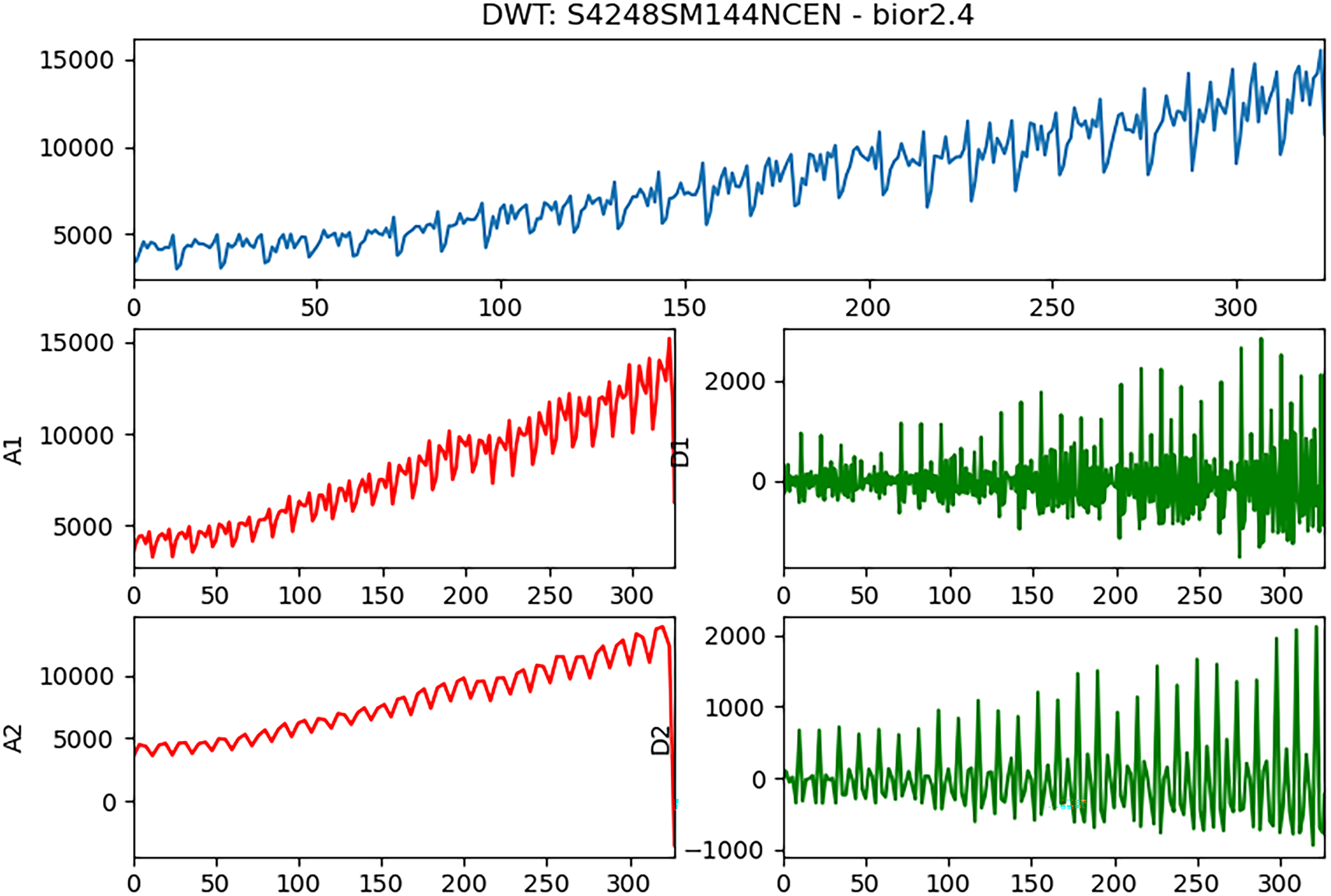
By applying DWT, the original time series can be decomposed into two components: the high-frequency (referred to as detail, denoted as D) and the low-frequency components (referred to as approximation, denoted as A).²⁷ This decomposition process can be repeated multiple times, with each subsequent decomposition being applied to the resulting low-frequency component. This iterative process builds a multilevel wavelet transform or a multiresolution representation. Figure 4 illustrates an example of implementing DWT on a time series using the bior 2.4 filter banks as the wavelet function with two levels of decomposition. Upon performing the two-level decomposition, it becomes apparent that the obtained frequency components (subsequences) exhibit relatively simple patterns and can be considered as either trend or periodic sequences, in contrast to the original time series, which typically contains complex patterns. These subsequences can be predicted using the same methods employed for trend or periodic time series. Subsequently, the predicted time series is reconstructed by employing the inverse DWT (IDWT) on these predicted subsequences.

Figure 4.

Example of decomposition with discrete wavelet transform (DWT) (A_n/D_n are the low-/high-frequency components of n-stage decomposition).

In the fourth section, the predictive results before and after decomposition will be compared.

The whole workflow

Based on the mentioned characteristics estimation and decomposition-based prediction method, the workflow can be organized as follows:

Data preprocessing

The raw data undergoes several preprocessing steps such as interpolating for missing values, normalization, and standardization.

Characteristics estimation

The preprocessed time series data is categorized into three types based on the proposed characteristics estimation: trend, periodic, and mixed.

Model selection and hyperparameter optimization

For the time series identified as trend or periodic, a model selection process is performed. This involves optimizing a range of time forecasting models using Optuna to tune their hyperparameters. The optimized models are then tested with the target time series data to select the best model. On the other hand, for the time series determined as mixed type, the proposed decomposition-based forecasting method is applied.

Experiments

In order to validate the proposed method in this article, a wide range of experiments have been carried out. Mean absolute percentage error (MAPE) is used as evaluation criteria, which is defined as

\begin{matrix} MAPE = \frac{100}{n} \sum_{i = 1}^{n} | \frac{\hat{y_{i}} - y_{i}}{y_{i}} | \end{matrix}

(6)

In the experiment, a closed loop forecasting mode is implemented, which simulates a normal engineering scenario. In this mode, the prediction for each subsequent time step in the sequence is made using the previous predictions as input, without relying on the true values.

All experimental data used below are obtained from Federal Reserve Economic Data, FRED. FRED is an online database consisting of more than 819,000 economic data time series from 110 national, international, public and private sources. All the used data can be downloaded from https://fred.stlouisfed.org/.

Experiments of hyperparameter optimization with Optuna

In this part, two typical periodic and trend time series are tested without and with hyperparameter automatic optimization. Figure 5 and Table 2 show the prediction performance comparison on periodic time series before and after hyperparameter optimization, while Figure 6 and Table 3 show the prediction performance comparison on trend time series.

Figure 5.

Prediction performance comparison before and after hyperparameter optimization (periodic time series). (a) DLinear before optimization. (b) DLinear after optimization. (c) N-BEATS before optimization. (d) N-BEATS after optimization. (e) N-HiTS (Neural Hierarchical Interpolation for Time-Series) before optimization. (f) N-HiTS after optimization. (g) NLinear before optimization. (h) NLinear after optimization. (i) Temporal Fusion Transformer (TFT) before optimization. (j) TFT after optimization.

Figure 6.

Prediction performance comparison before and after hyperparameter optimization (trend time series).

Table 2.

Prediction performance (MAPE) comparison before and after hyperparameter optimization (periodic time series).

	DLinear	N-BEATS	N-HiTS	NLinear	TFT
Before optimization	6.87%	7.02%	4.30%	5.73%	17.98%
After optimization	3.21%	4.44%	3.29%	2.86%	9.99%

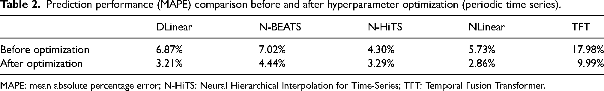
MAPE: mean absolute percentage error; N-HiTS: Neural Hierarchical Interpolation for Time-Series; TFT: Temporal Fusion Transformer.

Table 3.

Prediction performance (MAPE) comparison before and after hyperparameter optimization (trend time series).

	DLinear	N-BEATS	N-HiTS	NLinear	Transformer
Before optimization	27.07%	3.75%	18.48%	7.06%	4.86%
After optimization	2.71%	2.23%	2.82%	2.68%	3.79%
After optimization	3.21%	4.44%	3.29%	2.86%	9.99%

MAPE: mean absolute percentage error; N-HiTS: Neural Hierarchical Interpolation for Time-Series.

It could be found, before hyperparameter optimization, some algorithms (e.g. TFT in Figure 5) cannot accurately predict the trend characteristics of periodic sequences, and some algorithms (e.g. DLinear, N-HiTS in Figure 6) cannot accurately predict the vibrating part for trending sequences. From above results in Figures 5 and 6, and Tables 2 and 3, performance improvements for both types of time series after hyperparameter automatic optimization are obvious.

Experiments for decomposition-based time series forecasting method

In order to validate the performance and effectiveness of the decomposition-based time series forecasting method for mixed type time series. Two examples are tested

Figures 7 and 9 present two cases of mixed-type time series, and Figures 8 and 10 show their decomposition results. From the results presented in Tables 4 and 5, it is evident that the proposed decomposition-based time series forecasting method consistently achieves the best performance in both cases. This outcome provides strong evidence for the effectiveness of this decomposition-based approach.

Figure 7.

Time series of mixed type (case 1).

Figure 8.

Decomposition results (case1, A_n/D_n are the low/high frequency components of n-stage decomposition).

Figure 9.

Time series of mixed type (case 2).

Models	TCN	DLinear	N-HiTS	GRU	NLinear	Decomposition
MAPE(%)	7.22	3.21	3.29	12.20	2.86	2.68

Model	TCN	DLinear	N-HiTS	GRU	NLinear	Decomposition
MAPE(%)	15.96	10.24	9.83	17.28	10.92	8.15

Train:Test	TCN	GRU	TFT	DLinear	N-HiTS	NLinear
9:1	2.59	1.01	1.69	0.72	0.71	2.41
8:2	7.35	1.21	4.65	2.65	0.91	2.01
7:3	8.51	4.61	7.36	3.86	1.14	4.29

Train:Test	TCN	GRU	TFT	DLinear	N-HiTS	NLinear
9:1	1.59	0.46	0.64	0.89	0.44	2.06
8:2	1.60	1.45	1.53	3.29	0.90	2.99
7:3	2.42	1.47	1.47	3.45	0.79	3.28

Train:Test	TCN	GRU	TFT	D-Linear	N-HiTS	N-Linear	Decomposition
9:1	9.45	8.78	7.49	17.43	7.01	27.64	5.88
8:2	16.15	15.89	15.12	22.03	12.22	17.19	9.78
7:3	19.72	13.03	10.74	22.99	9.86	25.20	8.33

Train:Test	TCN	GRU	TFT	D-Linear	N-HiTS	N-Linear
9:1	4.34	4.17	8.59	3.81	3.37	3.96
8:2	8.02	6.49	9.75	3.77	4.17	6.60
7:3	7.29	5.42	7.30	4.26	4.04	4.06

Train:Test	TCN	GRU	TFT	DLinear	N-HiTS	N-Linear
9:1	6.37	7.30	7.26	4.28	4.20	4.73
8:2	7.19	7.54	7.37	4.26	4.80	4.77
7:3	8.17	8.18	8.47	7.92	6.44	8.69

Train:Test	TCN	GRU	TFT	DLinear	N-HiTS	NLinear	Decomposition
9:1	15.96	17.28	17.65	10.24	9.83	10.92	8 . 15
8:2	23.66	22.37	22.64	23.83	20.27	24.21	19.54
7:3	23.10	20.65	20.30	20.66	16.53	23.01	13.24

Train:Test	TCN	GRU	TFT	DLinear	N-HiTS	NLinear
9:1	1.40	1.14	1.55	1.07	1.46	0.86
8:2	2.92	1.93	2.89	1.83	2.07	1.45
7:3	4.31	2.57	3.03	3.40	3.17	3.26

Train:Test	TCN	GRU	TFT	DLinear	N-HiTS	NLinear
9:1	9.65	5.04	4.56	10.35	4.61	12.43
8:2	13.31	8.74	7.58	13.78	5.91	12.60
7:3	13.57	8.15	7.70	16.85	7.05	11.99

Train:Test	TCN	GRU	TFT	DLinear	N-HiTS	NLinear	Decomposition
9:1	24.07	13.84	12.96	10.90	9.40	17.04	7 . 88
8:2	19.49	22.95	18.15	19.33	15.30	20.78	13.59
7:3	25.66	27.03	18.75	20.54	17.30	22.07	16.21

Figure 10.
Decomposition results (case2, A_n/D_n are the low-/high-frequency components of n-stage decomposition).

Table 4.
Prediction performance comparison between single model and decomposition-based method (case 1).

Models TCN DLinear N-HiTS GRU NLinear Decomposition

MAPE(%) 7.22 3.21 3.29 12.20 2.86 2.68

GRU: Gated Recurrent Unit; MAPE: mean absolute percentage error; N-HiTS: Neural Hierarchical Interpolation for Time-Series.

Table 5.
Prediction performance comparison between single model and decomposition-based method (case 2).

Model TCN DLinear N-HiTS GRU NLinear Decomposition

MAPE(%) 15.96 10.24 9.83 17.28 10.92 8.15

GRU: Gated Recurrent Unit; MAPE: mean absolute percentage error; N-HiTS: Neural Hierarchical Interpolation for Time-Series.

Performance validation with different kinds of time series

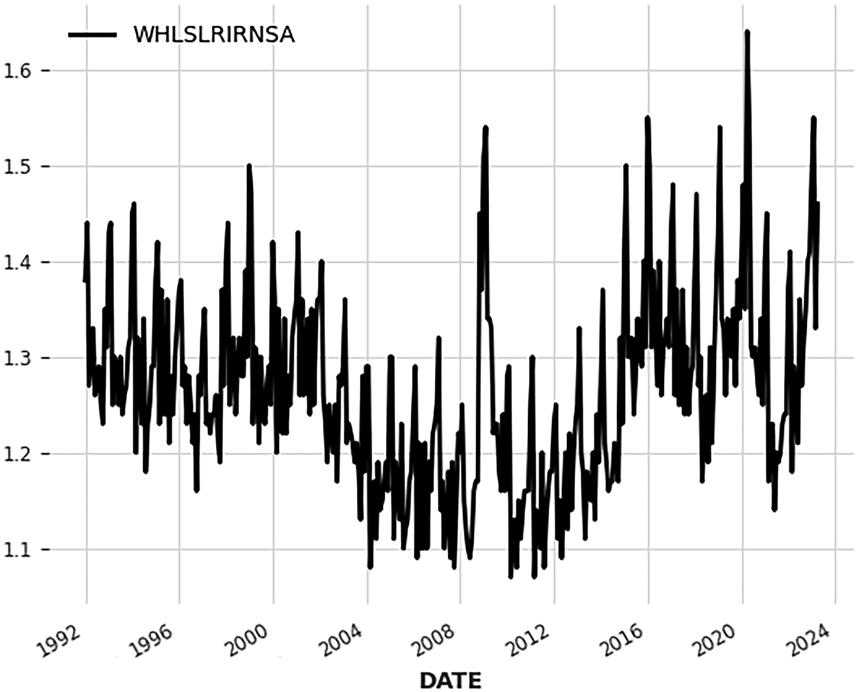
In this part of the study, a wide range of time series with different lengths and types are tested using the proposed hybrid time series forecasting method. Figures 11 to 19 present the time series used for testing, the length and r value of each series are marked in the figure title. However, considering the performance and time required for hyperparameter optimization, the search range of models is restricted to DLinear, N-HiTS, and NLinear. To evaluate the method's performance across various forecasting horizons, each test case includes three different ratios of train set to test set, which mimic short-term, medium-term, and long-term forecasts.

Figure 11.
Short time series 1(length: 96, r = 0.1293).

Figure 12.
Short time series 2 (length: 85, r = 8.6987).

Figure 13.
Short time series 3 (length: 96, r = 1.5835).

Figure 14.
Medium time series 1 (length: 376, r = 0.0170).

Figure 15.
Medium time series 2 (length: 376, r = 6.3662).

Figure 16.
Medium time series 3 (length: 376, r = 6.3662).

Figure 17.
Long time series 1 (length: 781, r = 0.0472).

Figure 18.
Long time series 2 (length: 1000, r = 3.6671).

Figure 19.
Long time series 3 (length: 553, r = 2.1231).

Case 1: short time series

Case 2: medium time series (lengths between 100 and 500)

Case 3: long time series (length over 500)

Based on the results presented in Tables 6 to 14, it is evident that the best results are consistently obtained with the forecasting methods within the restricted search range for each test case and ratio of training to test set. This finding holds true when the time series exhibit periodicity or trends. Moreover, when dealing with mixed type time series, the proposed decomposition-based time series forecasting method consistently outperforms other methods, regardless of the specific case or ratio of training to test set. This observation aligns with the results obtained in the experiments discussed in the “Experiments for decomposition-based time series forecasting method” section. Based on these consistent findings, it can be asserted that the hybrid method proposed in this article demonstrates the best overall performance.

Table 6.
Performance (MAPE%) comparison 1 (bold font indicates the best result).

Train:Test TCN GRU TFT DLinear N-HiTS NLinear

9:1 2.59 1.01 1.69 0.72 0.71 2.41

8:2 7.35 1.21 4.65 2.65 0.91 2.01

7:3 8.51 4.61 7.36 3.86 1.14 4.29

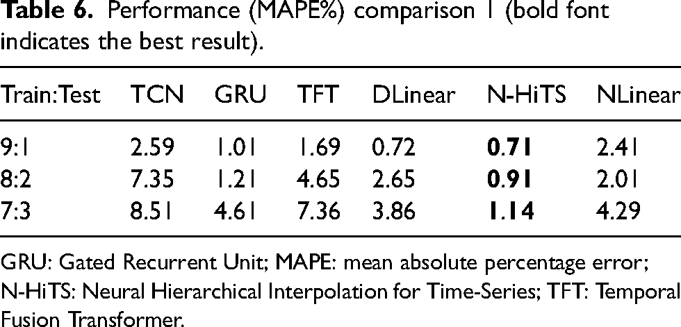
GRU: Gated Recurrent Unit; MAPE: mean absolute percentage error; N-HiTS: Neural Hierarchical Interpolation for Time-Series; TFT: Temporal Fusion Transformer.

Table 7.
Performance (MAPE%) comparison 2 (bold font indicates the best result).

Train:Test TCN GRU TFT DLinear N-HiTS NLinear

9:1 1.59 0.46 0.64 0.89 0.44 2.06

8:2 1.60 1.45 1.53 3.29 0.90 2.99

7:3 2.42 1.47 1.47 3.45 0.79 3.28

GRU: Gated Recurrent Unit; MAPE: mean absolute percentage error; N-HiTS: Neural Hierarchical Interpolation for Time-Series; TFT: Temporal Fusion Transformer.

Table 8.
Performance (MAPE%) comparison 3 (bold font indicates the best result).

Train:Test TCN GRU TFT D-Linear N-HiTS N-Linear Decomposition

9:1 9.45 8.78 7.49 17.43 7.01 27.64 5.88

8:2 16.15 15.89 15.12 22.03 12.22 17.19 9.78

7:3 19.72 13.03 10.74 22.99 9.86 25.20 8.33

GRU: Gated Recurrent Unit; MAPE: mean absolute percentage error; N-HiTS: Neural Hierarchical Interpolation for Time-Series; TFT: Temporal Fusion Transformer.

Table 9.
Performance (MAPE%) comparison 4 (bold font indicates the best result).

Train:Test TCN GRU TFT D-Linear N-HiTS N-Linear

9:1 4.34 4.17 8.59 3.81 3.37 3.96

8:2 8.02 6.49 9.75 3.77 4.17 6.60

7:3 7.29 5.42 7.30 4.26 4.04 4.06

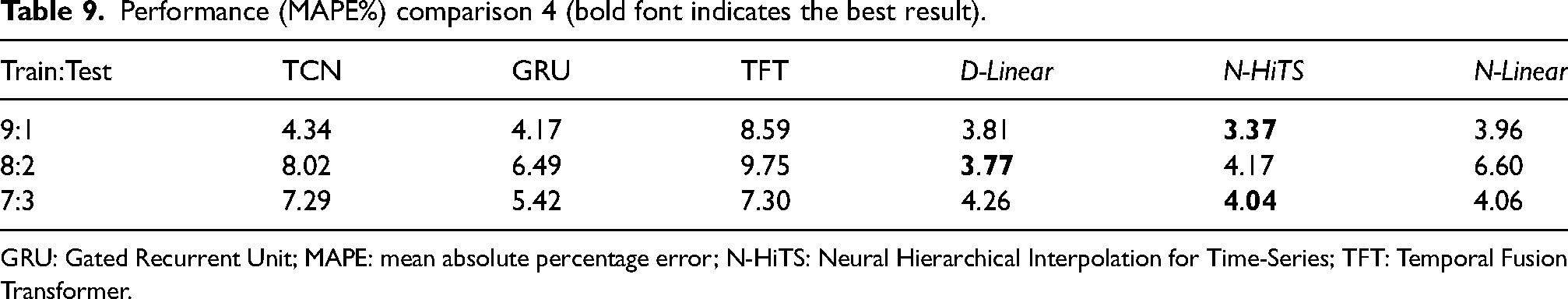
GRU: Gated Recurrent Unit; MAPE: mean absolute percentage error; N-HiTS: Neural Hierarchical Interpolation for Time-Series; TFT: Temporal Fusion Transformer.

Table 10.
Performance (MAPE%) comparison 5 (bold font indicates the best result).

Train:Test TCN GRU TFT DLinear N-HiTS N-Linear

9:1 6.37 7.30 7.26 4.28 4.20 4.73

8:2 7.19 7.54 7.37 4.26 4.80 4.77

7:3 8.17 8.18 8.47 7.92 6.44 8.69

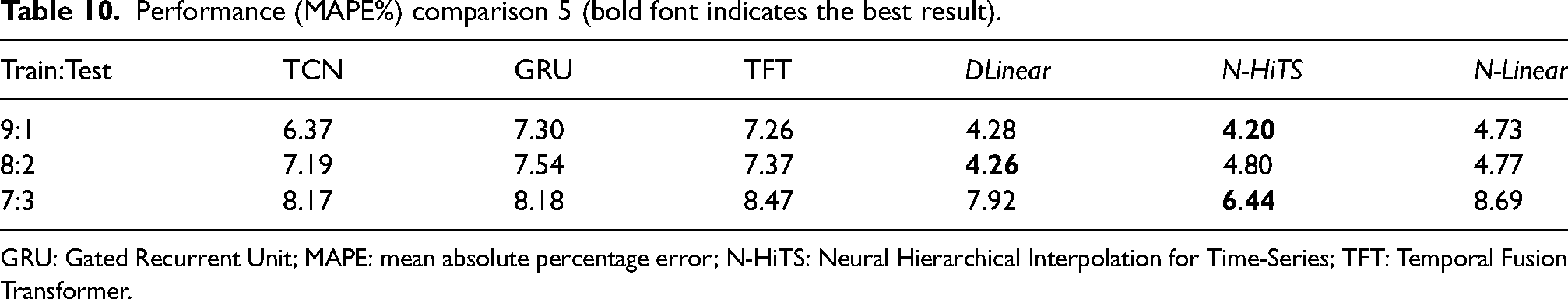
GRU: Gated Recurrent Unit; MAPE: mean absolute percentage error; N-HiTS: Neural Hierarchical Interpolation for Time-Series; TFT: Temporal Fusion Transformer.

Table 11.
Performance (MAPE%) comparison 6 (bold font indicates the best result).

Train:Test TCN GRU TFT DLinear N-HiTS NLinear Decomposition

9:1 15.96 17.28 17.65 10.24 9.83 10.92 8 . 15

8:2 23.66 22.37 22.64 23.83 20.27 24.21 19.54

7:3 23.10 20.65 20.30 20.66 16.53 23.01 13.24

GRU: Gated Recurrent Unit; MAPE: mean absolute percentage error; N-HiTS: Neural Hierarchical Interpolation for Time-Series; TFT: Temporal Fusion Transformer.

Table 12.
Performance (MAPE%) comparison 7 (bold font indicates the best result).

Train:Test TCN GRU TFT DLinear N-HiTS NLinear

9:1 1.40 1.14 1.55 1.07 1.46 0.86

8:2 2.92 1.93 2.89 1.83 2.07 1.45

7:3 4.31 2.57 3.03 3.40 3.17 3.26

GRU: Gated Recurrent Unit; MAPE: mean absolute percentage error; N-HiTS: Neural Hierarchical Interpolation for Time-Series; TFT: Temporal Fusion Transformer.

Table 13.
Performance (MAPE%) comparison 8 (bold font indicates the best result).

Train:Test TCN GRU TFT DLinear N-HiTS NLinear

9:1 9.65 5.04 4.56 10.35 4.61 12.43

8:2 13.31 8.74 7.58 13.78 5.91 12.60

7:3 13.57 8.15 7.70 16.85 7.05 11.99

GRU: Gated Recurrent Unit; MAPE: mean absolute percentage error; N-HiTS: Neural Hierarchical Interpolation for Time-Series; TFT: Temporal Fusion Transformer.

Table 14.
Performance (MAPE%) comparison 9 (bold font indicates the best result).

Train:Test TCN GRU TFT DLinear N-HiTS NLinear Decomposition

9:1 24.07 13.84 12.96 10.90 9.40 17.04 7 . 88

8:2 19.49 22.95 18.15 19.33 15.30 20.78 13.59

7:3 25.66 27.03 18.75 20.54 17.30 22.07 16.21

GRU: Gated Recurrent Unit; MAPE: mean absolute percentage error; N-HiTS: Neural Hierarchical Interpolation for Time-Series; TFT: Temporal Fusion Transformer.

In the above experiments, TFT (transform-based time series forecasting) is a method that is also evaluated alongside the proposed hybrid method. It is observed that TFT performs slightly lower in most cases compared to the hybrid method. However, due to the large number of weights and hyperparameters involved, the process of hyperparameter optimization for TFT is time-consuming and requires significant computational resources. The inclusion of TFT in the model search range was not carried out because of the long training time associated with it. Considering the practicality and efficiency of forecasting methods, it was decided to restrict the search range to models that could be trained and optimized within reasonable time limits.

Conclusion

To address the time series forecasting needs of logistic activities in intelligent manufacturing and to develop a behavior model of digital twin for logistics planning and operation, a hybrid time series forecasting method has been proposed. This method incorporates several tricks and techniques designed specifically for constructing an effective forecasting model. The experiments conducted to validate the proposed method demonstrate its high performance across a wide range of time series prediction problems, while also exhibiting low resource requirements and fast computation speed.

In current work, the value of r and the choice of wavelet function are mainly determined with experiment, which could be improved in the further work by introducing self-adaptive method.

Footnotes

Declaration of conflicting interests

The authors declared no potential conflicts of interest with respect to the research, authorship, and/or publication of this article.

Funding

The authors received no financial support for the research, authorship, and/or publication of this article.

ORCID iD

Tang Tang

References

1.
Han Z , Zhao, J, Leung, H, Ma, KF and Wang, W. A review of deep learning models for time series prediction. IEEE Sensors J 2019; 21: 7833–7848.

2.
Coelho F Relvas S Barbosa-Póvoa AP . Simulation-based decision support tool for in-house logistics: the basis for a digital twin. Comput Ind Eng 2021; 153: 107094.

3.
Agalianos K , Ponis ST, Aretoulaki E, et al. Discrete event simulation and digital twins: review and challenges for logistics. Procedia Manuf 2020; 51: 1636–1641.

4.
Park KT Son YH Noh SD . The architectural framework of a cyber physical logistics system for digital-twin-based supply chain control. Int J Prod Res 2021; 59: 5721–5742.

5.
Kaiblinger A Woschank M . State of the art and future directions of digital twins for production logistics: a systematic literature review. Appl Sci 2022; 12: 669.

6.
Pappas SS , Ekonomou L, Karampelas P, et al. Electricity demand load forecasting of the Hellenic power system using an ARMA model. Electr Power Syst Res 2010; 80: 256–264.

7.
Khashei M Bijari M . A novel hybridization of artificial neural networks and ARIMA models for time series forecasting. Appl Soft Comput 2011; 11: 2664–2675.

8.
Wang L , Zou H, Su J, et al. An ARIMA-ANN hybrid model for time series forecasting. Syst Res Behav Sci 2013; 30: 244–259.

9.
Doucoure B Agbossou K Cardenas A . Time series prediction using artificial wavelet neural network and multi-resolution analysis: application to wind speed data. Renewable Energy 2016; 92: 202–211.

10.
Gers FA Schmidhuber J Cummins F . Learning to forget: continual prediction with LSTM. Neural Comput 2000; 12: 2451–2471.

11.
Cho K , “Learning phrase representations using RNN encoder-decoder for statistical machine translation.” arXiv preprint arXiv:1406.1078 2014.

12.
Bai S Zico Kolter J Koltun V . “An empirical evaluation of generic convolutional and recurrent networks for sequence modeling.” arXiv preprint arXiv:1803.01271 2018.

13.
Oreshkin BN , Carpov D, Chapados N, et al. “N-BEATS: Neural basis expansion analysis for interpretable time series forecasting.” arXiv preprint arXiv:1905.10437 2019.

14.
Zeng A , Chen M, Zhang L, et al. Are transformers effective for time series forecasting? Proc AAAI Conf Artif Intell 2023; 37(9): 11121-11128. doi:https://doi.org/10.1609/aaai.v37i9.26317

15.
Challu C , Olivares K G, Oreshkin B N, et al. NHITS: Neural Hierarchical Interpolation for Time Series Forecasting. Proc AAAI Conf Artif Intell 2023; 37(6): 6989–6997. doi:https://doi.org/10.1609/aaai.v37i6.25854

16.
Vaswani A , Attention is all you need. Adv Neural Inf Process Syst 2017.

17.
Lim B , Arık S Ö, Loeff N, et al. Temporal fusion transformers for interpretable multi-horizon time series forecasting. Int J Forecast 2021; 37: 1748–1764.

18.
Zhou H , Zhang S, Peng J, et al. Informer: beyond efficient transformer for long sequence time-series forecasting. Proc AAAI Conf Artif Intell 2021; 35(12): 11106–11115. doi:https://doi.org/10.1609/aaai.v35i12.17325

19.
Wu H , Xu J, Wang J, et al. Autoformer: decomposition transformers with auto-correlation for long-term series forecasting. Adv Neural Inf Process Syst 2021; 34: 22419–22430.

20.
Cirstea R-G , Guo C, Yang B, et al. “Triformer: triangular, variable-specific attentions for long sequence multivariate time series forecasting–full version.” arXiv preprint arXiv:2204.13767 2022.

21.
Akiba T , Sano S, Yanase T, et al. Optuna: a next-generation hyperparameter optimization framework. In: Proceedings of the 25th ACM SIGKDD International Conference on Knowledge Discovery & Data Mining. 2019.

22.
Huang NE , Shen Z, Long S R, et al. The empirical mode decomposition and the Hilbert spectrum for nonlinear and non-stationary time series analysis. Proc Royal Soc London. Ser A Math Phys Eng Sci 1998; 454.1971: 903–995.

23.
Lin D-C , Guo Z L, An F P, et al. Elimination of end effects in empirical mode decomposition by mirror image coupled with support vector regression. Mech Syst Signal Process 2012; 31: 13–28.

24.
Qingjie Z Huayong Z Lincheng S . A new method for mitigation of end effect in empirical mode decomposition. In: 2010 2nd International Asia Conference on Informatics in Control, Automation and Robotics (CAR 2010), 2010. IEEE. Vol. 1.

25.
Shensa MJ . The discrete wavelet transform: wedding the a trous and Mallat algorithms. IEEE Trans Signal Process 1992; 40: 2464–2482.

26.
Chaovalit P , Gangopadhyay A, Karabatis G, et al. Discrete wavelet transform-based time series analysis and mining. ACM Computing Surveys (CSUR) 2011; 43: 1–37.

27.
Jawerth B Sweldens W . An overview of wavelet based multiresolution analyses. SIAM Rev 1994; 36: 377–412.

Research on time forecasting model in digital twin for logistic activity in intelligent manufactory

Abstract

Keywords

Introduction

Related works

Time series forecasting models

Traditional predictive model

Deep learning predictive model

N-BEATS

DLinear

N-HiTS

Transformer

Optuna hyperparameter optimization

A novel time forecasting model

Characteristics estimation

Time series forecasting method based on decomposition

The whole workflow

Experiments

Experiments of hyperparameter optimization with Optuna

Experiments for decomposition-based time series forecasting method

Performance validation with different kinds of time series

Conclusion

Footnotes

Declaration of conflicting interests

Funding

ORCID iD

References