Mixed variational formulation for frictional contact problem in electro-elasticity

Abstract

We consider a mathematical model that describes the frictional contact of a piezoelectric body with an electrically conductive foundation. The material’s behavior is described by means of an electroelastic constitutive law, the contact is bilateral and associated with Trescas law of dry friction. We derive a mixed variational formulation of the problem, which is in the form of a coupled system for the displacement field, the electric potential, and a Lagrange multiplier. Then we prove the existence of a unique weak solution to the model by combining saddle-point theory and the fixed-point technique. Moreover, we present an efficient algorithm for approximating the weak solution for the contact problem, including friction and electrical contact conditions. We conclude by a numerical example that illustrates the applicability of the model.

Introduction

Smart materials have significant promise in many structural applications and are widely employed as switches and actuators in many engineering systems, including radioelectronics, electroacoustics, and measurement equipment. By utilizing direct and reverse piezoelectric effects, piezoelectric materials are used as both actuators and sensors in the construction of these structures. Of particular importance for many piezoelectric materials, such as ceramics, are piezoelectric effects. Therefore, it may not be possible to predict the electromechanical behavior without considering these effects. Contact problems involving piezoelectric materials have received considerable attention recently in the mathematical literature. Therefore, static frictional contact problems for electro-elastic materials, with or without the assumption that the foundation is electrically conductive, were studied by Benkhira et al., ¹ Gamorski and Migòrski, ² Matei, ³ Matei and Mircea, ⁴ Migorski et al., ⁵ Lerguet et al., ⁶ Hüeber et al. ⁷ and Sofonea and Matei ⁸ , and the references therein. According to Benkhira et al.^9–12 and Essoufi et al., ¹³ numerical approximations of variational inequalities using the alternating direction method of multiplier (ADMM) involving linear and nonlinear piezoelectric materials have been studied. The aim of this article is twofold. The first one consists in introducing a model that describes a frictional contact problem between a piezoelectric body and an electrically conductive foundation. Under the small deformations hypothesis, the process is supposed to be static, and the contact is modeled with bilateral conditions, a regularized electrical conductivity conditions, and the friction follows Tresca’s law. A mixed variational problem involving Lagrange multiplier is used in the analysis of the considered model.

Our second aim is to describe an ADMM for numerically resolving the frictional contact problem with regularized electrical conductivity condition. The process is based on separating the linear electro-elasticity contact subproblem from the friction conditions, to this end we introduce auxiliary unknowns. Then, to improve the problem’s conditioning, we apply the ADMMs to the appropriate augmented Lagrangian functional, resulting in a iterative method with a linear electro-elasticity problem as the main subproblem and auxiliary unknowns are explicitly calculated. Finally, some numerical results are shown to illustrate the applicability and robustness of this approach.

The reset of the article is structured as follows: The frictional contact process of the piezoelectric body is modeled in the “Statement of the problem” section, along with some preliminary data assumptions. In the “Mixed variational formulation” section, the mixed variational formulation is driven, utilizing a coupled system for the displacement field, electric potential, and Lagrange multiplier. We then state our existence and uniqueness result, Theorem 1, and provide a proof of it that combines saddle-point theory and the mixed-point technique. In the “Alternating direction method of multipliers” section, we examine two-dimensional test problems and numerically demonstrate the theoretical result.

Statement of the problem

We suppose that an electro-elastic body occupies in its reference configuration a set $\mathrm{\Omega }\subset {\mathbb{R}}^d,d=2,3$ . $\mathrm{\Omega }$ is supposed to be open, bounded, with a sufficiently regular boundary $\mathrm{\Gamma }$ and the outward unit normal vector on $\mathrm{\Gamma }$ is denoted by $\nu$ . Moreover, $\mathrm{\Gamma }$ is assumed to be divided into three open disjoint parts ${\mathrm{\Gamma }}_1,{\mathrm{\Gamma }}_2$ , and ${\mathrm{\Gamma }}_3$ , on the one hand, and a partition of ${\mathrm{\Gamma }}_1\cup {\mathrm{\Gamma }}_2$ into two open parts ${\mathrm{\Gamma }}_a$ and ${\mathrm{\Gamma }}_b$ , on the other hand, such that meas ${\mathrm{\Gamma }}_1>0$ and meas ${\mathrm{\Gamma }}_a>0$ . We assume that the body is clamped on ${\mathrm{\Gamma }}_1$ , so the displacement field vanishes there. A volume force of density $f_0$ and volume electric charge of density $q_0$ acts in $\mathrm{\Omega }$ . A surface traction of density $f_2$ are applied on ${\mathrm{\Gamma }}_2$ , a surface electric charge of density $q_2$ acts on ${\mathrm{\Gamma }}_b$ and the electrical potential vanishes on ${\mathrm{\Gamma }}_a$ . Moreover, the body is in frictional contact with an electrically thermally conductive obstacle over the contact surface ${\mathrm{\Gamma }}_3$ , we assume that its potential is maintained at ${\phi }_F$ . Here and below, to simplify the notation, we do not indicate the dependence of various functions on the spatial variable $\mathit{x}\in \overline{\mathrm{\Omega }}$ , the summation convention over repeated indices is used and the index following a comma indicates a partial derivative. We assume that the process is static and let ${\mathbb{S}}^d$ be the space of second order symmetric tensors on ${\mathbb{R}}^d$ or equivalently, the space of real symmetric matrices of order $d$ , that is $\mathrm{\forall }\mathit{u},\mathit{v}\in {\mathbb{R}}^d$ , $\mathrm{\forall }\mathit{\sigma }$ , $\mathit{\tau }\in {\mathbb{S}}^d$ , $\mathit{u}\cdot \mathit{v}=u_i\cdot v_i$ , $\Vert \mathit{v}\Vert =(\mathit{v}\cdot \mathit{v}{)}^{1/2}$ , and $\mathit{\sigma }\cdot \mathit{\tau }={\sigma }_{ij}\cdot {\tau }_{ij},$ $\Vert \mathit{\tau }\Vert =(\mathit{\tau }\cdot \mathit{\tau }{)}^{1/2}$ . We also use the notations for normal and tangential components of displacement vector and stress: $v_{\nu }=\mathit{v}\cdot \mathit{\nu }$ , ${\mathit{v}}_{\tau }=\mathit{v}-v_{\nu }\mathit{\nu }$ , ${\sigma }_{\nu }=(\mathit{\sigma }\mathit{\nu })\cdot \mathit{\nu }$ , ${\mathit{\sigma }}_{\tau }=\mathit{\sigma }\mathit{\nu }-{\sigma }_{\nu }\mathit{\nu }$ , where $\mathit{\nu }$ denote the outward normal vector on $\mathrm{\Gamma }$ . Throughout the article, we adopt the following notation: $\mathit{u}:\mathrm{\Omega }\to {\mathbb{R}}^d$ for the displacement field, $\mathit{\sigma }:\mathrm{\Omega }\to {\mathbb{S}}^d$ $\mathit{\sigma }=({\sigma }_{ij})$ for the stress tensor. Moreover, let $\mathit{\epsilon }(\mathit{u})=({\epsilon }_{ij}(\mathit{u}))$ denote the linearized strain tensor given by ${\epsilon }_{ij}(\mathit{u})=$ $\frac{1}{2}(u_{i,j}+u_{j,i})$ . $\mathbf{D}:\mathrm{\Omega }\to {\mathbb{R}}^d$ denote the electric displacements field, $\mathbf{E}(\phi )=-\mathrm{\nabla }\phi$ denote the electric vector field, where $\phi :\mathrm{\Omega }\to \mathbb{R}$ is an electrical potential.

As a description of the electro-elastic material, the constitutive law can be written as follows:

$$\mathit{\sigma }=\mathfrak{F}\mathit{\epsilon }(\mathit{u})-\mathcal{E}*\mathbf{E}(\phi ),\mathbf{D}=\mathcal{E}\mathit{\epsilon }(\mathit{u})+\mathit{\beta }\mathbf{E}(\phi )\text{ in }\mathrm{\Omega }$$

(1)

in which the operator $\mathfrak{F}=(f_{ijkl})$ is the elasticity tensor, $\mathcal{E}=(e_{ijk}):\mathrm{\Omega }\times {\mathbb{S}}^d\to {\mathbb{R}}^d$ is the piezoelectric tensor, and $\mathit{\beta }=({\beta }_{ij}):\mathrm{\Omega }\times {\mathbb{R}}^d\to {\mathbb{R}}^d$ is the electric permittivity tensor. We use here ${\mathcal{E}}^{*}$ to denote the transpose of the tensor $\mathcal{E}$ given by $\mathcal{E}\mathit{\sigma }\mathit{v}=\mathit{\sigma }\mathcal{E}*\mathit{v}$ for all $\mathit{\sigma }\in {\mathbb{S}}^d,\mathit{v}\in {\mathbb{R}}^d$ .

The model under consideration is obtained from the equilibrium equations

$$\mathrm{Div}\mathit{\sigma }+{\mathit{f}}_0=0,\mathrm{div}\mathbf{D}=q_0\text{in }\mathrm{\Omega }$$

(2)

where $\mathrm{Div}\mathit{\sigma }=({\sigma }_{ij,j}),$ and $\mathrm{Div}\mathbf{D}=({\mathrm{D}}_{j,j})$ .

To complete the mechanical model, we prescribe the boundary conditions

$$\mathit{u}=0\text{on }{\mathrm{\Gamma }}_1,\mathit{\sigma }\mathit{\nu }={\mathit{f}}_2\text{on }{\mathrm{\Gamma }}_2,\phi =0\text{on }{\mathrm{\Gamma }}_a$$

(3)

On the surface ${\mathrm{\Gamma }}_3$ , we model the frictional contact, in the case of a perfect electrically foundation with bilateral condition, and Tresca’s friction law, that is,

$$u_{\nu }=0\text{ on }{\mathrm{\Gamma }}_3$$

(4)

$$\begin{array}{c}\Vert {\mathit{\sigma }}_{\tau }\Vert \le S\\ \Vert {\mathit{\sigma }}_{\tau }\Vert <S\Rightarrow {\mathit{u}}_{\tau }=0\\ \Vert {\mathit{\sigma }}_{\tau }\Vert =-S\frac{{\mathit{u}}_{\tau }}{\Vert {\mathit{u}}_{\tau }\Vert }\Rightarrow {\mathit{u}}_{\tau }\ne 0\end{array}\}\text{, on }{\mathrm{\Gamma }}_3$$

(5)

$$\mathbf{D}\cdot \mathit{\nu }=k_e{\varphi }_L(\phi -{\phi }_F)\text{, on }{\mathrm{\Gamma }}_3$$

(6)

Conditions (4) to (6) represent, respectively, the bilateral contact condition, Tresca’s friction law in which $S$ is the stress limit and the electrical contact condition, in which $k_e>0$ is the electrical conductivity constant and $\delta >0$ is a small parameter and $L$ is a large positive constant (see Lerguet et al. ⁶ ), and ${\varphi }_L$ is the truncation function, used to control the boundedness of $(\phi -{\phi }_F)$ . In applications, we chose ${\varphi }_L(\phi -{\phi }_F)=(\phi -{\phi }_F)$ (see Benkhira et al. ¹ and Lerguet et al. ⁶ ).

To conclude, the frictional contact problem under consideration can be stated as follows:

Problem (P). Find a displacement field $\mathit{u}:\mathrm{\Omega }\to {\mathbb{R}}^d$ , a stress field $\mathit{\sigma }:\mathrm{\Omega }\to {\mathbb{S}}^d$ , an electric potential $\phi :\mathrm{\Omega }\to \mathbb{R}$ and an electric displacement field $\mathbf{D}:\mathrm{\Omega }\to {\mathbb{R}}^d$ satisfying (1) to (6).

In next section, we give a weak formulation with dual Lagrange multipliers of the problem (P).

Mixed variational formulation

To derive the variational formulation of the Problem (P), we consider the real Hilbert spaces $H=L^2(\mathrm{\Omega }{)}^d$ , $H_1=H^1(\mathrm{\Omega }{)}^d$ , and $\mathcal{H}=\{\mathit{\sigma }=({\sigma }_{ij}),{\sigma }_{ij}={\sigma }_{ji}\in L^2(\mathrm{\Omega })\}$ . We also introduce the displacement field space $V$ and the potential electric field space $W$ such that

$$\begin{array}{rl}V& =\{\mathit{v}\in H_1;\mathit{v}=0\text{ on }{\mathrm{\Gamma }}_1\}\\ W& =\{\psi \in H^1(\mathrm{\Omega });\psi =0\text{ on }{\mathrm{\Gamma }}_a\}\end{array}$$

It follows from the Korn’s inequality that the previous spaces endowed with the inner products $(\mathit{u},\mathit{v}{)}_V=(\mathit{\epsilon }(\mathit{u}),\mathit{\epsilon }(\mathit{v}){)}_{\mathcal{H}}$ , $(\phi ,\psi {)}_W=$ $(\phi ,\psi {)}_{H^1(\mathrm{\Omega })}$ are Hilbert spaces.

Let $H_{\mathrm{\Gamma }}=H^{\frac{1}{2}}(\mathrm{\Gamma }{)}^d$ and let us denote by $\gamma$ the Sobolev trace operator, $\gamma :H_1\to H_{\mathrm{\Gamma }}$ , the mapping $\gamma$ is a linear, continuous, and compact operator. In addition, we recall that there exists a linear and continuous operator:

$$Z:H_{\mathrm{\Gamma }}\to H_1,\gamma (Z(\mathit{w}))=\mathit{w}\mathrm{\forall }\mathit{w}\in H_{\mathrm{\Gamma }}$$

(7)

The operator $Z$ is called the right inverse of the operator $\gamma$ . Let note also $H_{{\mathrm{\Gamma }}_3}=\gamma (V)$ , the space of traces on ${\mathrm{\Gamma }}_3$ , and its dual, $H_{{\mathrm{\Gamma }}_3}^{\mathrm{\prime }}$ .

The following assumptions are made on the given data:

• $(h_1)$

$\mathfrak{F}=({\mathfrak{F}}_{ijlk})$ satisfies ${\mathfrak{F}}_{ijlk}={\mathfrak{F}}_{ijkl}={\mathfrak{F}}_{lkij}\in L^{\mathrm{\infty }}(\mathrm{\Omega })$ and ${\mathfrak{F}}_{ijlk}{\epsilon }_{ij}{\epsilon }_{lk}\ge m_{\mathfrak{F}}\Vert \epsilon {\Vert }^2\mathrm{\forall }\epsilon \in {\mathbb{S}}^d$ , where $m_{\mathfrak{F}}$ is a positive constant.

$(h_2)$

$\mathcal{E}=(e_{ijk})$ satisfies $e_{ijk}=e_{ikj}\in L^{\mathrm{\infty }}(\mathrm{\Omega })$

$(h_3)$

$\beta =({\beta }_{ij})$ satisfies ${\beta }_{ij}={\beta }_{ji}\in L^{\mathrm{\infty }}(\mathrm{\Omega })$ and ${\beta }_{ij}{E}_i{E}_j\ge$ $m_{\beta }\Vert E{\Vert }^2\mathrm{\forall }E\in {\mathbb{R}}^d$ , where $m_{\beta }$ is a positive constant.

$(h_4)$

The stress limit satisfies $S\in L^{\mathrm{\infty }}({\mathrm{\Gamma }}_3),S\ge 0$ .

$(h_5)$

${\mathit{f}}_0\in L^2(\mathrm{\Omega }{)}^d,{\mathit{f}}_2\in L^2({\mathrm{\Gamma }}_2{)}^d,q_0\in L^2(\mathrm{\Omega }),q_2\in L^2({\mathrm{\Gamma }}_b)$ .

Using Riesz’s representation theorem, we define $\mathit{f}\in V$ , $q_e\in W$ as follows:

$$\begin{array}{rl}(\mathit{f},\mathit{v}{)}_V& ={\int }_{\mathrm{\Omega }}{\mathit{f}}_0\cdot \mathit{v}dx+{\int }_{{\mathrm{\Gamma }}_2}{\mathit{f}}_2\cdot \mathit{v}da\mathrm{\forall }\mathit{v}\in V\\ (q_e,\xi {)}_W& ={\int }_{\mathrm{\Omega }}{q}_0\cdot \xi dx+{\int }_{{\mathrm{\Gamma }}_2}{q}_2\cdot \xi da\mathrm{\forall }\xi \in W\end{array}$$

We also define the mapping $\ell :V\times W\times W\to \mathbb{R}$ given by the following equation:

$$\ell (\mathit{u},\phi ,\xi )={\int }_{{\mathrm{\Gamma }}_3}{k}_e{\varphi }_L(\phi -{\phi }_F)\xi da$$

Let us define the bilinear forms:

$$\begin{array}{rl}& A_m:V\times V\to \mathbb{R},(A_m\mathit{u},\mathit{v}{)}_V=(\mathfrak{F}\mathit{\epsilon }(\mathit{u}),\mathit{\epsilon }(\mathit{v}){)}_{\mathcal{H}}\\ & B_m:W\times V\to \mathbb{R},(B_m\phi ,\mathit{v}{)}_V=(\mathcal{E}*\mathrm{\nabla }\phi ,\mathit{\epsilon }(\mathit{v}){)}_H\\ & A_e:W\times W\to \mathbb{R},(A_e\phi ,\xi {)}_W=(\mathit{\beta }\mathrm{\nabla }\phi ,\mathrm{\nabla }\xi {)}_H\\ & B_e:V\times W\to \mathbb{R},(B_e\mathit{u},\xi {)}_W=-(\mathcal{E}\mathit{\epsilon }(\mathit{u}),\mathrm{\nabla }\xi {)}_H\end{array}$$

Due to Green’s formula, for regular functions $\mathit{u}$ and $\phi$ satisfying (1) to (3), we get for all $(\mathit{v},\phi )\in V\times W$

$$(A_m\mathit{u},\mathit{v}{)}_V+(B_m\phi ,\mathit{v}{)}_V=(\mathit{f},\mathit{v}{)}_V+{\int }_{{\mathrm{\Gamma }}_3}{\mathit{\sigma }}_{\tau }\cdot {\mathit{v}}_{\tau }da$$

(8)

$$(A_e\phi ,\xi {)}_W+(B_e\mathit{u},\xi {)}_W+\ell (\mathit{u},\phi ,\xi )=(q_e,\xi {)}_W$$

(9)

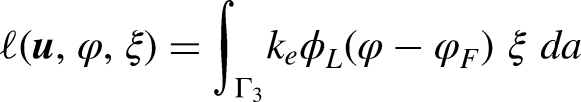
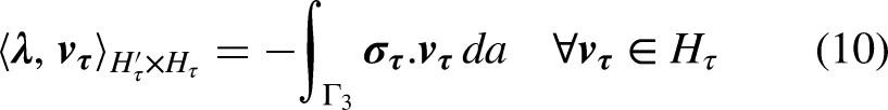
Let $\mathit{\lambda }\in H_{\tau }^{\mathrm{\prime }}$ be the Lagrangian multipliers given by the following equation:

$$⟨\mathit{\lambda },{\mathit{v}}_{\mathit{\tau }}{⟩}_{H_{\tau }^{\mathrm{\prime }}\times H_{\tau }}=-{\int }_{{\mathrm{\Gamma }}_3}{\mathit{\sigma }}_{\mathit{\tau }}.{\mathit{v}}_{\mathit{\tau }}da\mathrm{\forall }{\mathit{v}}_{\mathit{\tau }}\in H_{\tau }$$

(10)

where $⟨\cdot ,\cdot {⟩}_{X^{\mathrm{\prime }}\times X}$ denote the duality pairing between $X^{\mathrm{\prime }}$ and $X$ . In addition, we define the bilinear form $b:V\times H_{\tau }^{\mathrm{\prime }}\to \mathbb{R}$ by the following equation:

$$b(\mathit{v},\mathit{\zeta })=⟨\mathit{\zeta },{\mathit{v}}_{\mathit{\tau }}{⟩}_{H_{\tau }^{\mathrm{\prime }}\times H_{\tau }}\mathrm{\forall }\mathit{v}\in V,\mathit{\zeta }\in H_{\tau }^{\mathrm{\prime }}$$

(11)

We introduce the following subset of $H_{\tau }^{\mathrm{\prime }}$ ,

$$\mathrm{\Lambda }=\{\mathit{\zeta }\in H_{\tau }^{\mathrm{\prime }};⟨\mathit{\zeta },{\mathit{v}}_{\mathit{\tau }}{⟩}_{H_{\tau }^{\mathrm{\prime }}\times H_{\tau }}\le {\int }_{{\mathrm{\Gamma }}_3}S\Vert {\mathit{v}}_{\mathit{\tau }}\Vert da\mathrm{\forall }\mathit{v}\in V\}$$

(12)

It is obvious that ${\mathbf{0}}_{H_{\tau }^{\mathrm{\prime }}}\in \mathrm{\Lambda }$ . Also, $\mathrm{\Lambda }$ is closed, convex subset, of the space $H_{\tau }^{\mathrm{\prime }}$ , and by (5) it is clear that $\mathit{\lambda }$ is an element of $\mathrm{\Lambda }$ . Moreover, by (5), we obtain

$$b(\mathit{u},\mathit{\lambda })={\int }_{{\mathrm{\Gamma }}_3}S\Vert {\mathit{u}}_{\mathit{\tau }}\Vert da$$

and, using the definition of the subset $\mathrm{\Lambda }$ , we get

$$b(\mathit{u},\mathit{\zeta })\le {\int }_{{\mathrm{\Gamma }}_3}S\Vert {\mathit{u}}_{\mathit{\tau }}\Vert da\mathrm{\forall }\mathit{\lambda }\in \mathrm{\Lambda }$$

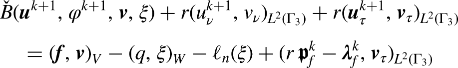
Thus, we are led to the following mixed variational formulation.

Problem (PV). Find $\mathit{u}\in V,\phi \in W$ and $\mathit{\lambda }\in \mathrm{\Lambda }$ such that

$$(A_m\mathit{u},\mathit{v}{)}_V+(B_m\phi ,\mathit{v}{)}_V+b(\mathit{v},\mathit{\lambda })=(\mathit{f},\mathit{v}{)}_V\mathrm{\forall }\mathit{v}\in V$$

(13)

$$(A_e\phi ,\xi {)}_W+(B_e\mathit{u},\xi {)}_W+\ell (\mathit{u},\phi ,\xi )=(q_e,\xi {)}_W\mathrm{\forall }\xi \in W$$

(14)

$$b(\mathit{u},\mathit{\zeta }-\mathit{\lambda })\le 0\mathrm{\forall }\mathit{\zeta }\in \mathrm{\Lambda }$$

(15)

Now, we can assert the following existence and uniqueness result.

Theorem 1

Assume that $(h_1)-(h_4)$ hold. Then, Problem (PV) has a unique solution $(\mathit{u},\phi )\in V\times W$ and $\mathit{\lambda }\in \mathrm{\Lambda }$ .

The proof of Theorem 1 will be carried out in several steps. In the first step, we consider the following product space: $X=V\times W$ . We equip the space $X$ with the canonical inner product denoted $(\cdot ,\cdot {)}_X$ and the associated norm $\Vert \cdot {\Vert }_X$ . On $H_{\tau }$ , we use the canonical product norm, denoted $\Vert \cdot {\Vert }_{H_{\tau }}$ . Also, we consider the operators $A:X\to X$ , $B:X\to X$ , the form $b:X\times H_{\tau }\to \mathbb{R}$ , the mapping $\tilde{\ell }:X\times X⟼W$ and the element ${\mathit{f}}_3\in X$ defined by the following equations:

$$\begin{array}{rl}& (A\mathit{x},\mathit{y}{)}_X=(A_m\mathit{u},\mathit{v}{)}_V+(A_e\phi ,\xi {)}_W\\ & (B\mathit{x},\mathit{y}{)}_X=(B_m\phi ,\mathit{v}{)}_V+(B_e\mathit{u},\xi {)}_W\\ & b(\mathit{y},\mathit{\lambda })=b(\mathit{v},\mathit{\lambda })\\ & \tilde{\ell }(\mathit{x},\mathit{y})=\ell (\phi ,\xi )\\ & {\mathit{f}}_3=(\mathit{f},q_e)\in X\end{array}$$

for all $\mathit{x}=(\mathit{u},\phi )\in X$ , $\mathit{y}=(\mathit{v},\xi )\in X$ , and $\mathit{\lambda }\in \mathrm{\Lambda }$ .

With these notation we consider the following mixed variational problem.

$\mathbf{P}\mathbf{r}\mathbf{o}\mathbf{b}\mathbf{l}\mathbf{e}\mathbf{m}\mathbf{(}\stackrel{\mathbf{~}}{\mathbf{P}\mathbf{V}}\mathbf{)}\mathbf{.}$ Find $\mathit{x}=(\mathit{u},\phi )\in X$ and $\mathit{\lambda }\in \mathrm{\Lambda }$ such that

$$(A\mathit{x},\mathit{y}{)}_X+(B\mathit{x},\mathit{y}{)}_X+\tilde{\ell }(\mathit{x},\mathit{y})+b(\mathit{y},\mathit{\lambda })=({\mathit{f}}_3,\mathit{y}{)}_X\mathrm{\forall }\mathit{y}=(\mathit{v},\xi )\in X$$

(16)

$$b(\mathit{x},\mathit{\zeta }-\mathit{\lambda })\le 0\mathrm{\forall }\mathit{\zeta }\in \mathrm{\Lambda }$$

(17)

It is easy to see that the following result holds:

Lemma 2

The functions $\mathit{u}$ , $\phi$ and $\mathit{\lambda }$ represent a solution to Problem (PV) if and only if the functions $\mathit{x}=(\mathit{u},\phi )$ , $\mathit{\lambda }$ represent a solution to Problem ( $\widetilde{PV}$ ). In addition, if $(\mathit{x},\mathit{\lambda })\in X\times \mathrm{\Lambda }$ is a solution of Problem ( $\widetilde{PV}$ ), then $(\mathit{x},\mathit{\lambda })\in K_1$ $\times (\mathrm{\Lambda }\cap K_2)$ , where

$$\begin{array}{rl}{K}_1& =\{\mathit{y}\in X;\Vert \mathit{y}{\Vert }_X\le \frac{1}{m_A}\Vert {\mathit{f}}_3{\Vert }_X\}\\ K_2& =\{\mathit{\zeta }\in \mathrm{\Lambda };\Vert \zeta {\Vert }_{H_{\tau }^{\mathrm{\prime }}}\le \frac{m_A+M_A}{m_b{m}_A}\Vert {\mathit{f}}_3{\Vert }_X\}\end{array}$$

Then, we study the properties of the operators $b(\cdot ,\cdot )$ . By an algebraic manipulations, we can demonstrate that there exist $M_b>0$ such that

$$b(\mathit{y},\mathit{\zeta })\le M_b\Vert \mathit{y}{\Vert }_X\Vert \mathit{\zeta }{\Vert }_{H_{\tau }^{\mathrm{\prime }}}\mathrm{\forall }\mathit{y}\in X,\mathit{\zeta }\in H_{\tau }^{\mathrm{\prime }}$$

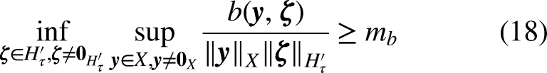
We also can prove that the bilinear form $b(\cdot ,\cdot )$ has the following inf-sup proprieties:

$$\underset{\begin{array}{c}\mathit{\zeta }\in H_{\tau }^{\mathrm{\prime }},\\ \mathit{\zeta }\ne {\mathbf{0}}_{H_{\tau }^{\mathrm{\prime }}}\end{array}}{inf}\underset{\begin{array}{c}\mathit{y}\in X,\\ \mathit{y}\ne {\mathbf{0}}_X\end{array}}{sup}\frac{b(\mathit{y},\mathit{\zeta })}{\Vert \mathit{y}{\Vert }_X\Vert \mathit{\zeta }{\Vert }_{H_{\tau }^{\mathrm{\prime }}}}\ge m_b$$

(18)

Indeed, by the definitions of $H_{\tau }^{\mathrm{\prime }}$ norm’s and the right inverse of the trace map, we have

$$\begin{array}{rl}\Vert \mathit{\zeta }{\Vert }_{H_{\tau }^{\mathrm{\prime }}}=& \underset{\begin{array}{c}\mathit{\omega }\in H_{\tau },\\ \mathit{\omega }\ne {\mathbf{0}}_{H_{\tau }}\end{array}}{sup}\frac{⟨\mathit{\zeta },\mathit{\omega }{⟩}_{H_{\tau }^{\mathrm{\prime }}\times H_{\tau }}}{\Vert \mathit{\omega }{\Vert }_{H_{\tau }}}\\ & \le c_1\underset{\begin{array}{c}\mathit{\omega }\in H_{\tau },\\ \mathit{\omega }\ne {\mathbf{0}}_{H_{\tau }}\end{array}}{sup}\frac{b(Z\mathit{\omega },\mathit{\zeta })}{\Vert Z\mathit{\omega }{\Vert }_X}\\ & \le c_1\underset{\begin{array}{c}\mathit{y}\in X,\\ \mathit{y}\ne {\mathbf{0}}_X\end{array}}{sup}\frac{b(\mathit{y},\mathit{\zeta })}{\Vert \mathit{y}{\Vert }_X}\end{array}$$

where $c_1>0$ , we can then take $m_b=\frac{1}{c_1}$ . Therefore, we deduce that

$$m_b\Vert \mathit{\zeta }{\Vert }_{H_{\tau }^{\mathrm{\prime }}}\le \underset{\begin{array}{c}\mathit{y}\in X,\\ \mathit{y}\ne {\mathbf{0}}_X\end{array}}{sup}\frac{b(\mathit{y},\mathit{\zeta })}{\Vert \mathit{y}{\Vert }_X}$$

Let $\mathcal{K}$ denote a closed convex set of $L^2({\mathrm{\Gamma }}_3)$ as follows:

$$\mathcal{K}=\{z\in L^2({\mathrm{\Gamma }}_3);\Vert z{\Vert }_{L^2({\mathrm{\Gamma }}_3)}\le \kappa \}$$

with $\kappa$ is a constant to be specified later. For every $z$ be an arbitrary fixed element of $L^2({\mathrm{\Gamma }}_3)$ , we define the function as follows:

$${\ell }_z(\mathit{y})={\int }_{{\mathrm{\Gamma }}_3}z\xi da\mathrm{\forall }\mathit{y}=(\mathit{v},\xi )\in X$$

We consider now the following intermediate problem:

$\mathbf{P}\mathbf{r}\mathbf{o}\mathbf{b}\mathbf{l}\mathbf{e}\mathbf{m}\mathbf{(}{\stackrel{\mathbf{~}}{\mathbf{P}\mathbf{V}}}_{\mathbf{z}}\mathbf{)}\mathbf{.}$ Find ${\mathit{x}}_z=({\mathit{u}}_z,{\phi }_z)\in X$ and ${\mathit{\lambda }}_z\in \mathrm{\Lambda }$ such that

$$(A{\mathit{x}}_z,\mathit{y}{)}_X+(B{\mathit{x}}_z,\mathit{y}{)}_X+{\tilde{\ell }}_z(\mathit{y})+b(\mathit{y},{\mathit{\lambda }}_z)=({\mathit{f}}_3,\mathit{y}{)}_X\mathrm{\forall }\mathit{y}=(\mathit{v},\xi )\in X$$

(19)

$$b({\mathit{x}}_z,\mathit{\zeta }-{\mathit{\lambda }}_z)\le 0\mathit{\zeta }\in \mathrm{\Lambda }$$

(20)

Let $z$ be an arbitrary fixed element of $\mathcal{K}$ . We are interested in determining the solvability of Problem ( ${\widetilde{PV}}_z$ ) using saddle-point theory applied to the functional $\mathcal{L}:X\times H_{\tau }^{\mathrm{\prime }}⟶\mathbb{R}$ defined by the following equation:

$$\mathcal{L}(\mathit{y},\mathit{\zeta })=\frac{1}{2}(A\mathit{y},\mathit{y}{)}_X+(\underset{=0}{\underbrace{B\mathit{y},\mathit{y}{)}_X}}-({\mathit{f}}_z,\mathit{y}{)}_X+b(\mathit{y},\mathit{\zeta })$$

where $({\mathit{f}}_z,\mathit{y}{)}_X=({\mathit{f}}_3,\mathit{y}{)}_X-{\tilde{\ell }}_z(\mathit{y})$ .

By standard arguments, it can be proved that: $({\mathit{x}}_{\mathit{z}},{\mathit{\lambda }}_{\mathit{z}})\in X\times \mathrm{\Lambda }$ is a solution of Problem ( ${\widetilde{PV}}_z$ ) if and only if it is a saddle-point the functional $\mathcal{L}$ .

Lemma 3

Problem ( ${\widetilde{PV}}_z$ ) has unique a solution $({\mathit{x}}_z,{\mathit{\lambda }}_{\mathit{z}})\in X\times \mathrm{\Lambda }$ .

Proof

The map $\mathit{y}\to \mathcal{L}(\mathit{y},\mathit{\zeta })$ is convex and lower semi-continuous for all $\mathit{\zeta }\in \mathrm{\Lambda }$ , and $\mathit{\zeta }\mapsto \mathcal{L}(\mathit{y},\mathit{\zeta })$ is concave and upper semi-continuous for all $\mathit{y}\in X$ . In addition, we note that

$$\begin{array}{rl}\mathcal{L}(\mathit{y},{\mathbf{0}}_{H_{\tau }^{\mathrm{\prime }}})=& \frac{1}{2}(A\mathit{y},\mathit{y}{)}_X-({\mathit{f}}_z,\mathit{y}{)}_X\\ & \le \left(\underset{\to \mathrm{\infty }\text{ as }\Vert \mathit{y}{\Vert }_X\to \mathrm{\infty }}{\underbrace{\frac{1}{2}(M_{\mathfrak{F}}+M_{\mathit{\beta }})\Vert \mathit{y}{\Vert }_X^2+\Vert {\mathit{f}}_3{\Vert }_X\Vert \mathit{y}{\Vert }_X+\mathfrak{C}\Vert \mathit{y}{\Vert }_X}}\right)\end{array}$$

with $M_{\mathfrak{F}}=\Vert \mathfrak{F}{\Vert }_{L^{\mathrm{\infty }}}$ , $M_{\mathit{\beta }}=\Vert \mathit{\beta }{\Vert }_{L^{\mathrm{\infty }}}$ and $\mathfrak{C}=\widetilde{c_0}\Vert z{\Vert }_{L^2({\mathrm{\Gamma }}_3)}$ . Thus, $\underset{\Vert \mathit{y}{\Vert }_X\to \mathrm{\infty }}{lim}\mathcal{L}(\mathit{y},{\mathbf{0}}_{H_{\tau }^{\mathrm{\prime }}})=\mathrm{\infty }$ . Let us prove now that

$$\underset{\begin{array}{c}\Vert \mathit{\zeta }{\Vert }_{H_{\tau }^{\mathrm{\prime }}}\to \mathrm{\infty },\\ \mathit{\zeta }\in \mathrm{\Lambda }\end{array}}{lim}\underset{\mathit{y}\in X}{inf}\mathcal{L}(\mathit{y},\mathit{\zeta })=-\mathrm{\infty }$$

(21)

To this end, let $\mathit{\zeta }$ be an arbitrary element in $\mathrm{\Lambda }$ , and let ${\mathit{x}}_{\mathit{\zeta }}$ be the unique solution of the equation:

$$(A{\mathit{x}}_{\mathit{\zeta }},\mathit{y}{)}_X+B({\mathit{x}}_{\mathit{\zeta }},\mathit{y}{)}_X+b({\mathit{x}}_{\mathit{\zeta }},\mathit{\zeta })=({\mathit{f}}_z,\mathit{y}{)}_X\mathrm{\forall }\mathit{y}\in X$$

(22)

guaranteed by the Lax-Milgram lemma. Since $(A\cdot ,\cdot {)}_X$ is symmetric and $B({\mathit{x}}_{\mathit{\zeta }},{\mathit{x}}_{\mathit{\zeta }}{)}_X=0$ , we can write

$$\underset{\mathit{y}\in X}{inf}\mathcal{L}(\mathit{y},\mathit{\zeta })=\frac{1}{2}(A{\mathit{x}}_{\mathit{\zeta }},{\mathit{x}}_{\mathit{\zeta }}{)}_X-({\mathit{f}}_z,{\mathit{x}}_{\mathit{\zeta }}{)}_X+b({\mathit{x}}_{\mathit{\zeta }},\mathit{\zeta })$$

Taking $\mathit{y}={\mathit{x}}_{\mathit{\zeta }}$ in (22), we get

$$-({\mathit{f}}_z,{\mathit{x}}_{\mathit{\zeta }}{)}_X+b({\mathit{x}}_{\mathit{\zeta }},\mathit{\zeta })=-(A{\mathit{x}}_{\mathit{\zeta }},{\mathit{x}}_{\mathit{\zeta }}{)}_X$$

Therefore

$$\underset{\mathit{y}\in X}{inf}\mathcal{L}(\mathit{y},\mathit{\zeta })=-\frac{1}{2}(A{\mathit{x}}_{\mathit{\zeta }},{\mathit{x}}_{\mathit{\zeta }}{)}_X$$

Due to the inf-sup property (18), we deduce that

$$m_b\Vert \mathit{\zeta }{\Vert }_{H_{\tau }^{\mathrm{\prime }}}\le \underset{\begin{array}{c}\mathit{y}\in X,\\ \mathit{y}\ne {\mathbf{0}}_X\end{array}}{sup}\frac{b(\mathit{y},\mathit{\zeta })}{\Vert \mathit{y}{\Vert }_X}$$

and by (22), we obtain

$$\begin{array}{rl}{m}_b\Vert \mathit{\zeta }{\Vert }_{H_{\tau }^{\mathrm{\prime }}}& \le \underset{\begin{array}{c}\mathit{y}\in X,\\ \mathit{y}\ne {\mathbf{0}}_X\end{array}}{sup}\frac{({\mathit{f}}_z,{\mathit{x}}_{\mathit{\zeta }}{)}_X-[(A{\mathit{x}}_{\mathit{\zeta }},\mathit{y}{)}_X+(B{\mathit{x}}_{\mathit{\zeta }},\mathit{y}{)}_X]}{\Vert \mathit{y}{\Vert }_X}\\ & \le \Vert {\mathit{f}}_3{\Vert }_X+\widetilde{c_0}\Vert z_2{\Vert }_{L^2({\mathrm{\Gamma }}_3)}+M_A\Vert {\mathit{x}}_{\mathit{\zeta }}{\Vert }_X\end{array}$$

where $M_A=M_{\mathit{F}}+M_{\mathit{\beta }}+M_{\mathcal{E}}$ . Therefore, there exist $c>0$ such that

$$\Vert \mathit{\zeta }{\Vert }_{H_{\tau }^{\mathrm{\prime }}}^2\le c(\Vert {\mathit{f}}_3{\Vert }_X^2+\Vert {\mathit{x}}_{\mathit{\zeta }}{\Vert }_X^2)$$

Furthermore, there exist $\tilde{c}>0$ such that

$$\underset{\mathit{y}\in X}{inf}\mathcal{L}(\mathit{y},\mathit{\zeta })\le -\tilde{c}(\Vert \mathit{\zeta }{\Vert }_{H_{\tau }^{\mathrm{\prime }}}^2-\Vert {\mathit{f}}_3{\Vert }_X^2)$$

Since $\mathit{\zeta }$ was arbitrarily fixed in $\mathrm{\Lambda }$ , passing to the limit as $\Vert \mathit{\zeta }{\Vert }_{H_{{\mathrm{\Gamma }}_3}^{\mathrm{\prime }}}\to \mathrm{\infty }$ leads us to (21). Consequently, we deduce that the functional $\mathcal{L}$ has at least one saddle-point, using an abstract result on saddle-point theory (see Matei ³ ). Since $({\mathit{x}}_z,{\mathit{\lambda }}_z)\in X\times \mathrm{\Lambda }$ is a solution of Problem ( ${\widetilde{PV}}_z$ ) if and only if it is a saddle-point the functional $\mathcal{L}$ , we conclude that Problem ( ${\widetilde{PV}}_z$ ) has at least one solution.

In fact, Problem ( ${\widetilde{PV}}_z$ ) has a unique solution $({\mathit{x}}_z,{\mathit{\lambda }}_{\mathit{z}})\in X\times \mathrm{\Lambda }$ . Indeed, let $({\mathit{x}}_z^1,{\mathit{\lambda }}_z^1)$ and $({\mathit{x}}_z^2,{\mathit{\lambda }}_z^2)$ be two solutions of Problem ( ${\widetilde{PV}}_z$ ). Keeping in mind (19),

$$(A{\mathit{x}}_z^1-A{\mathit{x}}_z^2,{\mathit{x}}_z^2-{\mathit{x}}_z^1{)}_X+(B{\mathit{x}}_z^1-B{\mathit{x}}_z^2,{\mathit{x}}_z^2-{\mathit{x}}_z^1{)}_X=b({\mathit{x}}_z^1,{\mathit{\lambda }}_z^2-{\mathit{\lambda }}_z^1)+b({\mathit{x}}_z^2,{\mathit{\lambda }}_z^1-{\mathit{\lambda }}_z^2)\le 0$$

Since $A$ is strongly monotone and

$$\begin{array}{rl}& (B{\mathit{x}}_z^1-B{\mathit{x}}_z^2,{\mathit{x}}_z^2-{\mathit{x}}_z^1{)}_X=0\\ & b({\mathit{x}}_z^1,{\mathit{\lambda }}_z^2-{\mathit{\lambda }}_z^1)+b({\mathit{x}}_z^2,{\mathit{\lambda }}_z^1-{\mathit{\lambda }}_z^2)\le 0\end{array}$$

we conclude that ${\mathit{x}}_z^1={\mathit{x}}_z^2$ . Moreover,

$$b(\mathit{y},{\mathit{\lambda }}_z^1-{\mathit{\lambda }}_z^2)=-[(A{\mathit{x}}_z^1-A{\mathit{x}}_z^2,\mathit{y}{)}_X+(B{\mathit{x}}_z^1-B{\mathit{x}}_z^2,\mathit{y}{)}_X]\mathrm{\forall }\mathit{y}\in X$$

By the inf-sup property (18), we conclude that ${\mathit{\lambda }}_z^1={\mathit{\lambda }}_z^2$ .

On the other hand, setting $\mathit{y}={\mathit{x}}_z$ in (19), $\mathit{\zeta }={\mathbf{0}}_{H_{\tau }^{\mathrm{\prime }}}$ in (20), we get that

$$(A{\mathit{x}}_z,{\mathit{x}}_z{)}_X+B({\mathit{x}}_z,{\mathit{x}}_{\mathit{z}}{)}_X+\widetilde{{\ell }_{\mathit{z}}}({\mathit{x}}_z)=({\mathit{f}}_3,{\mathit{x}}_z{)}_X-b({\mathit{x}}_z,{\mathit{\lambda }}_z)$$

with $(B{\mathit{x}}_z,{\mathit{x}}_z{)}_X=0$ and $-b({\mathit{x}}_z,{\mathit{\lambda }}_z)\le 0$ .

Since the operator $A:X\to X$ is strongly monotone and using the Cauchy-Schwarz inequality, we can write

$$m_A\Vert \mathit{x}{\Vert }_X^2\le (\Vert {\mathit{f}}_3{\Vert }_X+\widetilde{c_0}\Vert z{\Vert }_{L^2({\mathrm{\Gamma }}_3)})\Vert \mathit{x}{\Vert }_X$$

(23)

with $m_A=min(m_{\mathfrak{F}},m_{\mathit{\beta }})$ , it follows that ${\mathit{x}}_z\in K_1$ . Moreover, using again the inf-sup property of the form $b(\cdot ,\cdot )$ combined with (19), we obtain

$$\begin{array}{rl}{m}_b\Vert {\mathit{\lambda }}_z{\Vert }_{H_{{\mathrm{\Gamma }}_3}^{\mathrm{\prime }}}& \le \underset{\begin{array}{c}\mathit{y}\in X,\\ \mathit{y}\ne {\mathbf{0}}_X\end{array}}{sup}\frac{({\mathit{f}}_3,\mathit{y}{)}_X-[(A{\mathit{x}}_z,\mathit{y}{)}_X+(B{\mathit{x}}_z,\mathit{y}{)}_X+{\tilde{\ell }}_z(\mathit{y})]}{\Vert \mathit{y}{\Vert }_X}\\ & \le \Vert {\mathit{f}}_3{\Vert }_X+M_A\Vert {\mathit{x}}_z{\Vert }_X+\widetilde{c_0}\Vert z{\Vert }_{L^2({\mathrm{\Gamma }}_3)}\end{array}$$

(24)

From (23) and (24), we have ${\mathit{\lambda }}_z\in K_2$ .

Thus, there exists a unique solution of Problem ( ${\widetilde{PV}}_z$ ), $({\mathit{x}}_z,{\mathit{\lambda }}_z)$ , such that

$${\mathit{x}}_z\in K_1\text{ and }{\mathit{\lambda }}_z\in \mathrm{\Lambda }\cap K_2$$

(25)

In this step, we consider the operator $\mathrm{T}:L_2({\mathrm{\Gamma }}_3)⟶L_2({\mathrm{\Gamma }}_3)$ , defined by the following equation:

$$\mathrm{T}z=k_e{\varphi }_L(\phi -{\phi }_F)$$

Lemma 4

Let $({\mathit{u}}_n{)}_n\subset V$ be a sequence weakly convergent to $\mathit{u}$ in $V$ as $n\to +\mathrm{\infty }$ .

For each $\mathit{\zeta }\in \mathrm{\Lambda }$ there exists a sequence $({\mathit{\zeta }}_n{)}_n\subset H_{\tau }^{\mathrm{\prime }}$ such that

$${\mathit{\zeta }}_n\in \mathrm{\Lambda }\text{and}\underset{n\to +\mathrm{\infty }}{lim inf}b({\mathit{u}}_n,{\mathit{\zeta }}_n-\mathit{\zeta })\ge 0$$

If ${\mathit{\zeta }}_n\in H_{\tau }^{\mathrm{\prime }}$ such that ${\mathit{\zeta }}_n\in \mathrm{\Lambda }$ and ${\mathit{\zeta }}_n\rightharpoonup \mathit{\zeta }$ in $H_{\tau }^{\mathrm{\prime }}$ as $n\to +\mathrm{\infty }$ , then $\mathit{\zeta }\in \mathrm{\Lambda }$ .

Proof

Let $({\mathit{u}}_n{)}_n\subset V$ be a sequence weakly convergent to $\mathit{u}$ in $V$ as $n\to +\mathrm{\infty }$ .

We take an element $\mathit{\zeta }\in \mathrm{\Lambda }$ , and we define $({\mathit{\zeta }}_n{)}_n\subset H_{\tau }^{\mathrm{\prime }}$ by the following equation:

$$\begin{array}{rl}{\displaystyle ⟨{\mathit{\zeta }}_n,\mathit{v}{⟩}_{H_{\tau }^{\mathrm{\prime }}\times H_{\tau }}}& ={\displaystyle {\int }_{{\mathrm{\Gamma }}_3}S\mathrm{\Psi }({\mathit{u}}_{n,\tau })\mathit{v}da{\displaystyle -{\int }_{{\mathrm{\Gamma }}_3}S\Vert {\mathit{u}}_{n,\tau }\Vert da}}\\ & +⟨\mathit{\zeta },{\mathit{u}}_{n,\tau }{⟩}_{H_{\tau }^{\mathrm{\prime }}\times H_{\tau }}\mathrm{\forall }\mathit{v}\in H_{\tau }\end{array}$$

(26)

where

$$\mathrm{\Psi }(r)=\{\begin{array}{cc}{\displaystyle \frac{r}{\Vert r\Vert }}& \text{if}r\ne 0\\ 0& \text{if}r=0\end{array}$$

Since $\mathit{\zeta }\in \mathrm{\Lambda }$ , we have

$$-{\int }_{{\mathrm{\Gamma }}_3}S\Vert {\mathit{u}}_{n,\tau }\Vert da+⟨\mathit{\zeta },{\mathit{u}}_{n,\tau }{⟩}_{H_{\tau }^{\mathrm{\prime }}\times H_{\tau }}\le 0$$

We deduce that, for each positive integer $n$ , we have ${\mathit{\zeta }}_n\in \mathrm{\Lambda }$ .

On the other hand, using (26), we get

$$⟨{\mathit{\zeta }}_n-\mathit{\zeta },{\mathit{u}}_n{⟩}_{H_{\tau }^{\mathrm{\prime }}\times H_{\tau }}={\int }_{{\mathrm{\Gamma }}_3}S(\Vert {\mathit{u}}_{n,\tau }\Vert -\Vert {\mathit{u}}_{n,\tau }\Vert )da=0$$

it follows that:

$$\underset{n\to +\mathrm{\infty }}{lim inf}b({\mathit{u}}_n,{\mathit{\zeta }}_n-\mathit{\zeta })=0$$

Consider a sequence $({\mathit{\zeta }}_n{)}_n\subset H_{\tau }^{\mathrm{\prime }}$ such that $({\mathit{\zeta }}_n{)}_n\in \mathrm{\Lambda }$ , where ${\mathit{\zeta }}_n\rightharpoonup \mathit{\zeta }$ in $H_{\tau }^{\mathrm{\prime }}$ as $n\to +\mathrm{\infty }$ . According to the definition in (12), we have the following equation:

$$⟨{\mathit{\zeta }}_n,{\mathit{v}}_{\tau }{⟩}_{H_{\tau }^{\mathrm{\prime }}\times H_{\tau }}\le {\int }_{{\mathrm{\Gamma }}_3}S\Vert {\mathit{v}}_{\tau }\Vert da\mathrm{\forall }\mathit{v}\in \mathcal{K}$$

Since ${\mathit{\zeta }}_n$ converges weakly to $\mathit{\zeta }$ in $H_{\tau }^{\mathrm{\prime }}$ as $n\to +\mathrm{\infty }$ , and by passing to the limit as $n\to +\mathrm{\infty }$ in the previous inequality, we get

$$⟨\mathit{\zeta },{\mathit{v}}_{\tau }{⟩}_{H_{\tau }^{\mathrm{\prime }}\times H_{\tau }}\le {\int }_{{\mathrm{\Gamma }}_3}S\Vert {\mathit{v}}_{\tau }\Vert da\mathrm{\forall }\mathit{v}\in \mathcal{K}$$

Therefore, $\mathit{\zeta }\in \mathrm{\Lambda }$ .

Lemma 5

The operator $\mathrm{T}$ has a least one fixed point.

Proof

First, we will prove that the operator $\mathrm{T}$ is weakly sequentially continuous, that is, for each $(z_n{)}_n\subset L^2({\mathrm{\Gamma }}_3)$ , $z_n\rightharpoonup z$ in $L^2({\mathrm{\Gamma }}_3)$ as $n\to +\mathrm{\infty }$ , we have that $\mathrm{T}{z}_n\rightharpoonup \mathrm{T}z$ in $L^2({\mathrm{\Gamma }}_3)$ as $n\to +\mathrm{\infty }$ . To this end, let $(z_n{)}_n\subset L^2({\mathrm{\Gamma }}_3)$ be a sequence such that $z_n\rightharpoonup z$ in $L^2({\mathrm{\Gamma }}_3)$ as $n\to +\mathrm{\infty }$ . We define ${\mathit{x}}_n={\mathit{x}}_{z_n}$ and ${\mathit{\lambda }}_n={\mathit{\lambda }}_{z_n}$ . Since $({\mathit{x}}_n{)}_n\subset K_1$ and $K_1$ is bounded, there exists a subsequence of the sequence $({\mathit{x}}_n{)}_n$ , denoted again by $({\mathit{x}}_n{)}_n$ , and an element $\tilde{\mathit{x}}\in L^2({\mathrm{\Gamma }}_3)$ such that ${\mathit{x}}_n\rightharpoonup \tilde{\mathit{x}}$ in $L^2({\mathrm{\Gamma }}_3)$ as $n\to +\mathrm{\infty }$ . Furthermore, since $({\mathit{\lambda }}_n{)}_n\subset K_2$ and $K_2$ is bounded, there exists a subsequence of $({\mathit{\lambda }}_n{)}_n$ , denoted again by $({\mathit{\lambda }}_n{)}_n$ , and an element $\tilde{\mathit{\lambda }}\in H_{\tau }^{\mathrm{\prime }}$ such that $({\mathit{\lambda }}_n{)}_n\rightharpoonup \tilde{\mathit{\lambda }}$ in $H_{\tau }^{\mathrm{\prime }}$ as $n\to +\mathrm{\infty }$ . Passing to the limit as $n\to +\mathrm{\infty }$ in (19), we find that

$$(A\tilde{\mathit{x}},\mathit{y}{)}_X+(B\tilde{\mathit{x}},\mathit{y}{)}_X+b(\mathit{y},\tilde{\mathit{\lambda }})=({\mathit{f}}_z,\mathit{y}{)}_X\mathrm{\forall }\mathit{y}\in X$$

(27)

Moreover, since ${\mathit{\lambda }}_n\in \mathrm{\Lambda }$ , using Lemma 4, we get that

$$\tilde{\mathit{\lambda }}\in \mathrm{\Lambda }$$

(28)

According to Lemma 4, there exits ${\mathit{\zeta }}_n\in \mathrm{\Lambda }$ such that

$$\underset{n\to +\mathrm{\infty }}{lim inf}b({\mathit{x}}_{ϵ,n},{\mathit{\zeta }}_n-\mathit{\zeta })\ge 0$$

also, we have

$$b({\mathit{x}}_n,{\mathit{\zeta }}_n-{\mathit{\lambda }}_n)\le 0$$

or, equivalently

$$b({\mathit{x}}_n,{\mathit{\zeta }}_n-\mathit{\zeta })+b({\mathit{x}}_n,\mathit{\zeta })\le b({\mathit{x}}_n,{\mathit{\lambda }}_n)$$

which implies that

$$\underset{n\to +\mathrm{\infty }}{lim inf}b({\mathit{x}}_n,{\mathit{\zeta }}_n-\mathit{\zeta })+b(\tilde{\mathit{x}},\mathit{\zeta })\le \underset{n\to +\mathrm{\infty }}{lim sup}b({\mathit{x}}_n,{\mathit{\lambda }}_n)$$

(29)

Note that

$$b({\mathit{x}}_n,{\mathit{\lambda }}_n)=({\mathit{f}}_z,{\mathit{x}}_n{)}_X-(A{\mathit{x}}_n,{\mathit{x}}_n{)}_X-\underset{=0}{\underbrace{(B{\mathit{x}}_n,{\mathit{x}}_n{)}_X}}$$

(30)

Since the bilinear form $(A\cdot ,\cdot )$ is symmetric, continuous, and $X$ -elliptic, the map $X\ni \mathit{y}\mapsto (A\mathit{y},\mathit{y}{)}_X\in \mathbb{R}$ is convex and continuous. Therefore, the map $X\ni \mathit{y}\mapsto (A\mathit{y},\mathit{y}{)}_X\in \mathbb{R}$ is weakly lower semi-continuous and

$$\begin{array}{rl}\underset{n\to +\mathrm{\infty }}{lim sup}b({\mathit{x}}_n,{\mathit{\lambda }}_n)& \le ({\mathit{f}}_z,\tilde{\mathit{x}}{)}_X-(A\tilde{\mathit{x}},\tilde{\mathit{x}}{)}_X\\ & =b(\tilde{\mathit{u}},\tilde{\mathit{\lambda }})\end{array}$$

(31)

Combining (29) to (31), we obtain

$$b(\tilde{\mathit{x}},\mathit{\zeta }-\tilde{\mathit{\lambda }})\le 0\text{,for all }\mathit{\zeta }\in \mathrm{\Lambda }$$

(32)

Keeping in mind (27), (28), and (32), we deduce that $(\tilde{\mathit{x}},\tilde{\mathit{\lambda }})$ is a solution of Problem ( ${\widetilde{PV}}_z$ ). As Problem ( ${\widetilde{PV}}_z$ ) has a unique solution $({\mathit{x}}_z,{\mathit{\lambda }}_z)$ , we conclude that $\tilde{\mathit{x}}={\mathit{x}}_z$ , and $\tilde{\mathit{\lambda }}={\mathit{\lambda }}_{\mathit{z}}$ . Consequently, $\mathrm{T}z$ is the unique weak limit of all weak convergent subsequences of the sequence $(\mathrm{T}{z}_n{)}_n$ . Therefore, the whole sequence $(\mathrm{T}{z}_n{)}_n$ converges weakly in $L^2({\mathrm{\Gamma }}_3)$ to $\mathrm{T}z$ as $n\to +\mathrm{\infty }$ .

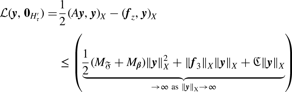
Let us now consider $z$ an element of $\mathcal{K}$ , we have $\Vert z{\Vert }_{L^2({\mathrm{\Gamma }}_3)}\le \kappa$ . On the other hand since ${\varphi }_L(\phi -{\phi }_F)\le L$ , it follows that:

$$\Vert \mathrm{T}z{\Vert }_{L^2({\mathrm{\Gamma }}_3)}\le meas({\mathrm{\Gamma }}_3{)}^{\frac{1}{2}}{k}_{e}L$$

Therefore, if we choose $\kappa =meas({\mathrm{\Gamma }}_3{)}^{\frac{1}{2}}{k}_{e}L$ , we can conclude that $\mathrm{T}$ is an operator of $\mathcal{K}$ in itself. Noting that $\mathcal{K}$ is a non-empty, convex, closed, and bounded subset of the reflexive space $L^2({\mathrm{\Gamma }}_3)$ , we can use a fixed-point theorem for weakly sequentially continuous maps, ¹⁴ to deduce that the operator $\mathrm{T}$ has at least one fixed point.

Proof of Lemma 2

Let us denote by $z*$ the fixed point of the operator $\mathrm{T}$ , we observe that the pair $({\mathit{x}}_{z*},{\mathit{\lambda }}_{z*})$ is a solution to Problem ( ${\widetilde{PV}}_z$ ) with $z=z*$ , the definition of $\mathrm{T}z$ , and ( ${\widetilde{PV}}_z$ ) prove that $({\mathit{x}}_{z*}$ , ${\mathit{\lambda }}_{z*})$ is solution of ( $\widetilde{PV}$ ).

To prove the uniqueness of the solution, assume that $({\mathit{x}}^{\mathbf{1}},{\mathit{\lambda }}^1)$ and $({\mathit{x}}^2,{\mathit{\lambda }}^2)$ are two solution of Problem ( $\widetilde{PV}$ ). It can be easily verified that ${\mathit{x}}^1={\mathit{x}}^2$ and ${\mathit{\lambda }}^1={\mathit{\lambda }}^2$ . Moreover, using (25) with $z=z*$ , we conclude that ${\mathit{x}}_{z*}\in K_1$ , and ${\mathit{\lambda }}_{z*}\in \mathrm{\Lambda }\cap K_2$ .

Next, let $(\mathit{x},\mathit{\lambda })\in X\times \mathrm{\Lambda }$ be a solution of Problem ( $\widetilde{PV}$ ). Let $\mathit{y}=\mathit{x}$ in (16) and let $\mathit{\zeta }={\mathbf{0}}_{H_{\tau }^{\mathrm{\prime }}}$ in (17). Thus

$$(A\mathit{x},\mathit{x}{)}_X\le ({\mathit{f}}_3,\mathit{x}{)}_X$$

Using the strong monotony of the operator $A$ and the Cauchy-Schwarz inequality, we deduce that $\mathit{x}\in K_1$ . Moreover, using again the inf-sup property of the form $b(\cdot ,\cdot )$ combined with (16), we obtain the following equation:

$$\begin{array}{rl}{m}_b\Vert \mathit{\lambda }{\Vert }_{H_{\tau }^{\mathrm{\prime }}}& \le \underset{\begin{array}{c}\mathit{y}\in X,\\ \mathit{y}\ne {\mathbf{0}}_X\end{array}}{sup}\frac{({\mathit{f}}_{\mathbf{3}},\mathit{y}{)}_X-(A\mathit{x},\mathit{y}{)}_X-(B\mathit{x},\mathit{y}{)}_X-\tilde{\ell }(\mathit{x},\mathit{y})}{\Vert \mathit{y}{\Vert }_X}\\ & \le \Vert {\mathit{f}}_3{\Vert }_X+m_A\Vert \mathit{x}{\Vert }_X\end{array}$$

Consequently, since $\mathit{x}\in K_1$ , we obtain $\mathit{\lambda }\in K_2$ .

Alternating direction method of multipliers

In this section, we give the computational algorithm in which use a variant of the augmented Lagrangian that uses partial updates, known as the alternating direction method of multipliers, to decompose the original problem into two sub-problems, solve them sequentially and update the double variables associated with a coupling constraint at each iteration. ¹⁵

For this purpose, an equivalent minimization problem must be introduced using the piezoelectric deformation energy functional due to non-frictional effects $J_n$ given by the following equation:

$$J_n(\mathit{v},\xi )=\frac{1}{2}\check{B}(\mathit{v},\xi ,\mathit{v},\xi )+{\ell }_n(\xi )-(\mathit{f},\mathit{v}{)}_V+(q,\xi {)}_W\mathrm{\forall }(\mathit{v},\xi )\in V\times W$$

where the bilinear symmetric form $\check{B}:V\times W\times V\times W\to \mathbb{R}$ is given by the following equation:

$$\check{B}(\mathit{v},\eta ,\mathit{w},\xi )=(\mathfrak{F}\mathit{\epsilon }(\mathit{u}),\mathit{\epsilon }(\mathit{v}){)}_{\mathcal{H}}+(\mathcal{E}*\mathrm{\nabla }\eta ,\mathit{\epsilon }(\mathit{w}){)}_H-(\mathit{\beta }\mathrm{\nabla }\eta ,\mathrm{\nabla }\xi {)}_H+(\mathcal{E}\mathit{\epsilon }(\mathit{v}),\mathrm{\nabla }\xi {)}_H$$

and

$${\ell }_n(\xi )=\ell ({\phi }_n,\xi ),j(\mathit{v})={\int }_{{\mathrm{\Gamma }}_3}S\Vert {\mathit{v}}_{\tau }\Vert da\mathrm{\forall }(\mathit{v},\xi )\in V\times W$$

Therefore, an equivalent constrained minimization problem can be formulated and it is as follows:

$$\begin{array}{rl}& \text{Find }(\mathit{u},\phi )\in K\times W\text{ such that }\\ & J_n(\mathit{u},\phi )+j(\mathit{u})\le J_n(\mathit{v},\xi )+j(\mathit{v})\mathrm{\forall }(\mathit{v},\xi )\in K\times W\end{array}$$

(33)

with $K$ be the set of admissible displacements

$$K=\{\mathit{v}\in V;v_{\nu }=0\text{on }{\mathrm{\Gamma }}_3\}$$

The quadratic functional $J_n$ is strictly convex and Gateaux differentiable on $V\times W$ . Moreover, the friction functional $j$ is convex and lower semi-continuous on $V$ , thus, there exists a unique solution to the minimization problem (33).

Let $\mathfrak{p}=({\mathfrak{p}}_f,{\mathfrak{p}}_c)$ , where ${\mathfrak{p}}_f$ (friction) and ${\mathfrak{p}}_c$ (contact) are auxiliary variables, we introduce the set

$$C=\{{\mathfrak{p}}_c\in L^2({\mathrm{\Gamma }}_3);{\mathfrak{p}}_c=0\text{on }{\mathrm{\Gamma }}_3\}$$

and the characteristic functional ${\mathrm{I}}_C:L^2({\mathrm{\Gamma }}_3)\to \mathbb{R}\cup \{+\mathrm{\infty }\}$ of the set $C$ , is defined by the following equation:

$${\mathrm{I}}_C({\mathfrak{p}}_c)=\{\begin{array}{cc}0,& \text{if}{\mathfrak{p}}_c\in C\\ +\mathrm{\infty },& \text{if}{\mathfrak{p}}_c\notin C\end{array}$$

It is easy to see that the problem giving in (33) is equivalent to the following constrained minimization problem:

Find $(\mathit{u},\phi )\in V\times W$ and $\mathfrak{p}=({\mathfrak{p}}_f,{\mathfrak{p}}_c)\in L^2({\mathrm{\Gamma }}_3{)}^2$ such that

$$J_n(\mathit{u},\phi )+j({\mathfrak{p}}_f)+{\mathrm{I}}_C({\mathfrak{p}}_c)\le J_n(\mathit{v},\xi )+j({\mathfrak{q}}_f)+I_C({\mathfrak{q}}_c)$$

(34)

$$\begin{array}{rl}& \begin{array}{c}{u}_{\nu }-{\mathfrak{p}}_c=0\\ {\mathit{u}}_{\tau }-{\mathfrak{p}}_f=0\end{array}\}\text{on }{\mathrm{\Gamma }}_3\end{array}$$

(35)

for all $(\mathit{v},\xi )\in V\times W$ and $\mathfrak{q}=({\mathfrak{q}}_f,{\mathfrak{q}}_c)\in L^2({\mathrm{\Gamma }}_3{)}^2$ .

From (34) and (35), the augmented Lagrangian functional ${\mathcal{L}}_r$ is defined over $V\times W\times L^2({\mathrm{\Gamma }}_3{)}^2\times L^2({\mathrm{\Gamma }}_3{)}^2$ by the following equation:

$$\begin{array}{rl}{\mathcal{L}}_r(\mathit{v},\xi ,\mathfrak{q};\mathit{\theta })& =J_n(\mathit{v},\xi )+j_n({\mathfrak{q}}_f)+{\mathrm{I}}_C({\mathfrak{q}}_c)+({\theta }_c,v_{\nu }-{\mathfrak{q}}_c{)}_{L^2({\mathrm{\Gamma }}_3)}\\ & +({\mathit{\theta }}_f,{\mathit{v}}_{\tau }-{\mathfrak{q}}_f{)}_{L^2({\mathrm{\Gamma }}_3)}+\frac{r}{2}\Vert v_{\nu }-{\mathfrak{q}}_c{\Vert }_{L^2({\mathrm{\Gamma }}_3)}^2\\ & +\frac{r}{2}\Vert {\mathit{v}}_{\tau }-{\mathfrak{q}}_f{\Vert }_{L^2({\mathrm{\Gamma }}_3)}^2\end{array}$$

(36)

where the constant $r>0$ is the penalty parameter and $\mathit{\theta }=({\mathit{\theta }}_f,{\theta }_c)$ . Since the functional $J_n+j$ is strictly convex, and the constraints (35) are linear, a saddle point of ${\mathcal{L}}_r$ exists, and it is the solution of the saddle-point problem

$$\{\begin{array}{cc}& \text{Find }((\mathit{u},\phi ,\mathfrak{p});\mathit{\lambda })\in V\times W\times L^2({\mathrm{\Gamma }}_3{)}^2\times L^2({\mathrm{\Gamma }}_3{)}^2\\ & \text{ such that}\\ & {\mathcal{L}}_r(\mathit{u},\phi ,\mathfrak{p};\mathit{\theta })\le {\mathcal{L}}_r(\mathit{u},\phi ,\mathfrak{p};\mathit{\lambda })\le {\mathcal{L}}_r(\mathit{v},\xi ,\mathfrak{q};\mathit{\lambda })\\ & \mathrm{\forall }((\mathit{v},\xi ,\mathfrak{q});\mathit{\theta })\in V\times W\times L^2({\mathrm{\Gamma }}_3{)}^2\times L^2({\mathrm{\Gamma }}_3{)}^2\end{array}$$

where we have set $\mathit{\lambda }=({\mathit{\lambda }}_f,{\lambda }_c)$ . Equivalently, $((\mathit{u},\phi ,\mathfrak{p});\mathit{\lambda })$ is the solution of the min-max problem

$$\underset{\mathit{\theta }}{max}\underset{(\mathit{v},\xi ,\mathfrak{q})}{min}{\mathcal{L}}_r(\mathit{v},\xi ,\mathfrak{q};\mathit{\theta })=\underset{(\mathit{v},\xi ,\mathfrak{q})}{min}\underset{\mathit{\theta }}{max}{\mathcal{L}}_r(\mathit{v},\xi ,\mathfrak{q};\mathit{\theta })$$

The method performs successive minimizations of the augmented Lagrangian functional ${\mathcal{L}}_r$ (36) in $\mathit{u}$ , $\phi$ and $\mathfrak{p}$ followed by the multiplier update, as follows, starting with ${\mathfrak{p}}^0$ and ${\mathit{\lambda }}^0$

$${\mathcal{L}}_r({\mathit{u}}^{k+1},{\phi }^{k+1},{\mathfrak{p}}^k;{\mathit{\lambda }}^k)=\underset{(\mathit{v},\xi )}{min}{\mathcal{L}}_r(\mathit{v},\xi ,{\mathfrak{p}}^k;{\mathit{\lambda }}^k)$$

(37)

$${\mathcal{L}}_r({\mathit{u}}^{k+1},{\phi }^{k+1},{\mathfrak{p}}^{k+1};{\mathit{\lambda }}^k)=\underset{\mathfrak{p}}{min}{\mathcal{L}}_r({\mathit{u}}^{k+1},{\phi }^{k+1},\mathfrak{q};{\mathit{\lambda }}^k)$$

(38)

$${\mathit{\lambda }}^{k+1}={\mathit{\lambda }}^k+r({\mathit{u}}^{k+1}-{\mathfrak{p}}^{k+1})$$

(39)

As the functional $(\mathit{v},\xi )\mapsto {\mathcal{L}}_r(\mathit{v},\xi ,\mathfrak{p};\mathit{\theta })$ is convex and differentiable, the solution of (37) is characterized by the Euler-Lagrange equation

$$\begin{array}{rl}& \check{B}({\mathit{u}}^{k+1},{\phi }^{k+1},\mathit{v},\xi )+r(u_{\nu }^{k+1},v_{\nu }{)}_{L^2({\mathrm{\Gamma }}_3)}+r({\mathit{u}}_{\tau }^{k+1},{\mathit{v}}_{\tau }{)}_{L^2({\mathrm{\Gamma }}_3)}\\ & =(\mathit{f},\mathit{v}{)}_V-(q,\xi {)}_W-{\ell }_n(\xi )+(r{\mathfrak{p}}_c^k-{\lambda }_c^k,v_{\nu }{)}_{L^2({\mathrm{\Gamma }}_3)}\\ & +(r{\mathfrak{p}}_f^k-{\mathit{\lambda }}_f^k,{\mathit{v}}_{\tau }{)}_{L^2({\mathrm{\Gamma }}_3)}\end{array}$$

The corresponding ADMM algorithm is presented in Algorithm 1. We iterate until the relative error on ${\mathit{u}}^k$ , ${\phi }^k$ and ${\mathfrak{p}}_f^k$ is sufficiently “small,” that is,

$$\frac{\Vert {\mathit{x}}^{k+1}-{\mathit{x}}^k{\Vert }_X^2+\Vert {\mathfrak{p}}_f^{k+1}-{\mathfrak{p}}_f^k{\Vert }_{L^2({\mathrm{\Gamma }}_3)}^2}{\Vert {\mathit{x}}^{k+1}{\Vert }_X^2+\Vert {\mathfrak{p}}_f^{k+1}{\Vert }_{L^2({\mathrm{\Gamma }}_3)}^2}<{ϵ}^2$$

(40)

with

$$\Vert {\mathit{x}}^{k+1}-{\mathit{x}}^k{\Vert }_X^2=\Vert {\mathit{u}}^{k+1}-{\mathit{u}}^k{\Vert }_V^2+\Vert {\phi }^{k+1}-{\phi }^k{\Vert }_W^2$$

Algorithm 1. ADMM algorithm for the constrained minimization problem.

Initialization. $r>0$ , ${\mathfrak{p}}_f^0$ and ${\mathit{\lambda }}^0=({\mathit{\lambda }}_f^0,{\lambda }_c^0)$ are given.

Iteration $k>0$ . Compute successively ${\mathit{u}}^{k+1}$ , ${\phi }^{k+1}$ , ${\mathfrak{p}}_f^{k+1}$ , and ${\mathit{\lambda }}^{k+1}=({\mathit{\lambda }}_f^{k+1},{\lambda }_c^{k+1})$ as follows:

Step 1. Find $({\mathit{u}}^{k+1},{\phi }^{k+1})\in V\times W$ such that

$$\begin{array}{rl}& \check{B}({\mathit{u}}^{k+1},{\phi }^{k+1},\mathit{v},\xi )+r(u_{\nu }^{k+1},v_{\nu }{)}_{L^2({\mathrm{\Gamma }}_3)}+r({\mathit{u}}_{\tau }^{k+1},{\mathit{v}}_{\tau }{)}_{L^2({\mathrm{\Gamma }}_3)}\\ & =(\mathit{f},\mathit{v}{)}_V-(q,\xi {)}_W-{\ell }_n(\xi )+(r{\mathfrak{p}}_f^k-{\mathit{\lambda }}_f^k,{\mathit{v}}_{\tau }{)}_{L^2({\mathrm{\Gamma }}_3)}\end{array}$$

Step 2. Compute the auxiliary friction variable

$${\mathfrak{p}}_f^{k+1}=\{\begin{array}{cc}{\displaystyle \frac{|{\mathit{\lambda }}_f^k+r{\mathit{u}}_{\tau }^{k+1}|-S}{r|{\mathit{\lambda }}_f^k+r{\mathit{u}}_{\tau }^{k+1}|}({\mathit{\lambda }}_f^k+r{\mathit{u}}_{\tau }^{k+1}),}& \mathrm{if}|{\mathit{\lambda }}_f^k+r{\mathit{u}}_{\tau }^{k+1}|>S\\ 0,& \mathrm{if}|{\mathit{\lambda }}_f^k+r{\mathit{u}}_{\tau }^{k+1}|\le S\end{array}$$

Step 3. Update the Lagrange multiplier

$${\mathit{\lambda }}_f^{k+1}={\mathit{\lambda }}_f^k+r({\mathit{u}}_{\tau }^{k+1}-{\mathfrak{p}}_f^{k+1})$$

With the above results, the solution method for the considered model is presented in Algorithm 2.

Algorithm 2. Solution for the iterative problem for the considered model.

Initialization. ${\mathit{u}}_0$ and ${\phi }_0$ are given.

Iteration $n\ge 0$ . Compute ${\mathit{u}}_{n+1}$ , ${\phi }_{n+1}$ and ${\ell }_{n+1}$ successively as follows:

Compute $({\phi }_{n+1})\in V\times W$ using Algorithm 1.

Update: ${\ell }_{n+1}(\xi )=\ell ({\mathit{u}}_{n+1},{\phi }_{n+1},\xi )$ .

Numerical experiments

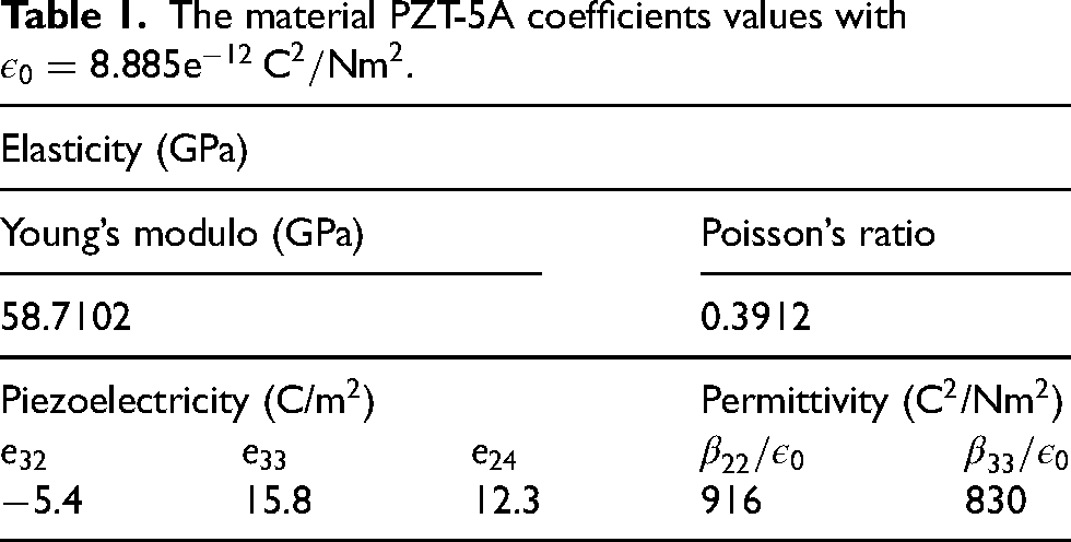
In this section, we will study the academic example of a parallelepiped bar which has the following dimensions: the height $h=1$ m and the length is equal to two times the height, with ${\mathrm{\Gamma }}_a={\mathrm{\Gamma }}_1=(\{0\}\times [0,1])$ , ${\mathrm{\Gamma }}_2={\mathrm{\Gamma }}_b=([0,2]\times \{1\})$ , and ${\mathrm{\Gamma }}_3=([0,2]\times \{0\})$ . The body force ${\mathit{f}}_0$ and the volume electric charge $q_0$ are assumed to be zero. The body is clamped on ${\mathrm{\Gamma }}_1$ and thus $\mathit{u}=0$ there. A surface traction and electric charge of densities ${\mathit{f}}_2(x)=(0,-2x){\text{N/m}}^2$ , $q_2(x)=0{\text{C/m}}^2$ , respectively, act on ${\mathrm{\Gamma }}_2$ . We suppose here that the behavior of the material is linear, the penalty parameter is $r=3.25\times E$ , the gap between ${\mathrm{\Gamma }}_3$ and the foundation is $\varrho =0$ and the characteristics of the material are those given in Table 1.

Table 1.

The material PZT-5A coefficients values with ${ϵ}_0=8.885{\text{e}}^{-12}{\text{C}}^2/{\text{Nm}}^2$ .

Elasticity (GPa)
Young’s modulo (GPa)			Poisson’s ratio
58.7102			0.3912
Piezoelectricity (C/m ${}^2$ )			Permittivity (C ${}^2$ /Nm ${}^2$ )
$e_{32}$	$e_{33}$	$e_{24}$	${\beta }_{22}/{ϵ}_0$	${\beta }_{33}/{ϵ}_0$
$-$ 5.4	15.8	12.3	916	830

Normal and tangential stress distributions on ${\mathrm{\Gamma }}_3$ are shown in Figure 1 while Figure 2 shows deformed configuration and electrical potential distribution with contact forces, in the case where the rigid foundation is conductive $(k_e=1)$ with $\mu =0.2$ .

Figure 1.

Normal and tangential stress distributions on ${\mathrm{\Gamma }}_3$ for $k_e=1$ and ${\phi }_F=$ 16 V.

Figure 2.

Deformed configuration and electrical potential distribution with contact forces (arrows) for $k_e=1$ and ${\phi }_F=$ 16 V.

For ${\phi }_F=$ 16 V and different values of $k_e$ , Figure 3 shows the electrical potential distribution on ${\mathrm{\Gamma }}_3$ , where can clearly see the influence of the electrical conductivity constant on the contact zone, ${\mathrm{\Gamma }}_3$ , electrical potential.

Figure 3.

Electrical potential distribution on ${\mathrm{\Gamma }}_3$ for ${\phi }_F=$ 16 V and different values of $k_e$ .

Conclusion

This article considers a model for static frictional contact between a piezoelectric body and an electrically conductive foundation. The contact is bilateral and was modeled using Tresca’s friction law and a regularized electrical conductivity condition. We proved the existence and the uniqueness of the weak solution using a mixed variational approach governed by dual Lagrange multipliers. The weak formulation we present is a new variational problem made up of two variational equations; this technique is appropriate for an efficient approximation of the weak solution. Indeed, as shown in the last portion of this article, we offer an efficient approach for approximating the problem’s weak solution. This algorithm was implemented in MATLAB using the ${\mathbb{P}}_1$ triangular finite element method. Finally, we have illustrated the performance of the proposed algorithm through a two-dimensional test problem. This test shows the continuous dependence of the weak solution of the piezoelectric contact Problem (P) with respect to the friction constant $S$ and the electric conductivity coefficient $k_e$ . These results are compatible with the electrical boundary condition we use on the contact surface and show the effect of the conductivity of the foundation on the process.