Binary spectral collocation method for the nonlinear Fokker-Planck equation

Abstract

A mixed Laguerre-Legendre spectral collocation schemes is constructed for initial-boundary value problem of the nonlinear Fokker-Planck nonhomogeneous equations and the linear Fokker-Planck homogeneous equation by using the Laguerre interpolation functions in velocity, and the Legendre interpolation functions in time, which is a bivariate Lagrange interpolation approximation function based on Legendre and Laguerre Gauss quadrature notes. The original problem is changed into a matrix equation and solved by Newton iteration. Numerical experiments show that the algorithm has high accuracy and efficiency.

Introduction

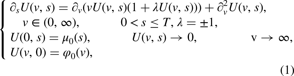
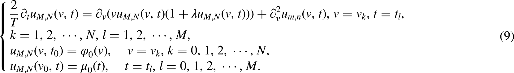
The nonlinear Fokker Planck equation is a class of partial differential equations that are commonly employed in diverse fields such as physics, mathematics, engineering, and other related fields, as exemplified in Reference. ¹ It plays a key role in describing many important processes in statistical mechanics, such as diffusion, transport, radiative transfer and fusion. However, due to its high-order, nonlinear, and coupling characteristics, solving the Fokker-Planck equation has always been a challenging problem. In the past three decades, with the rapid development of computer technology, the spectral method has become an important method for numerical simulation of some classical mathematical and physical equations, such as the Burgers equation, the KdV equation, and the Klein-Gordon equation (see, e.g. Refs.^2–12). Therefore, it is also interesting to consider the initial-boundary value problem using spectral methods. Then the considered problem is as follows:

$$\{\begin{array}{c}{\mathrm{\partial }}_{s}U(v,s)={\mathrm{\partial }}_v(vU(v,s)(1+\lambda U(v,s)))+{\mathrm{\partial }}_v^{2}U(v,s),\\ v\in (0,\mathrm{\infty }),0<s\le T,\lambda =\pm 1,\\ U(0,s)={\mu }_0(s),U(v,s)\to 0,\mathrm{v}\to \mathrm{\infty },0\le s\le T\\ U(v,0)={\phi }_0(v),v\in [0,\mathrm{\infty }).\end{array}$$

(1)

where $v,U(v,t)$ represent the velocity of the particles, the density of probability, respectively.

Some authors have studied the initial value problem of the above equation (see Refs.^13–15), but the work on the mixed problem has not been seen yet. On the other hand, in the aforementioned literature, the difference scheme is usually used in the time t direction, which leads to a serious imbalance between the nodes used in the velocity direction and the time direction, which greatly increases the work. To balance the nodes in velocity or space and time, some authors have considered time-space spectral collocation methods (see Refs.^16–18). The pseudo-spectral method is more desirable in practical calculations because it is easier to implement and saves the work of dealing with nonlinear terms. ⁴ The spectral collocation method is an effective technique for solving nonlinear equations. ¹⁹ Since the nonlinear Fokker Planck equation contains a variable coefficient term $vU(v,s)$ , it is more suitable to numerically solve by binary spectral collocation method.

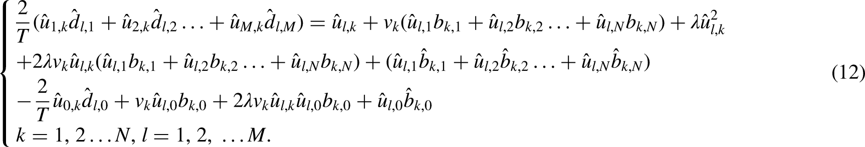
In this article, a mixed Laguerre-Legendre spectral collection scheme is proposed. The Laguerre spectral collocation method is used in velocity direction, which uses Laguerre interpolation functions based on Laguerre Gaussian quadrature nodes, and the Legendre spectral collocation method is used in time direction, which uses the Lagrange interpolation polynomial based on Legendre Gaussian quadrature points. By substituting binary interpolation polynomials into the original equation, a nonlinear systems is obtained, which can be solved with the Newton iteration.

Lagrange interpolation polynomials and its differential matrix

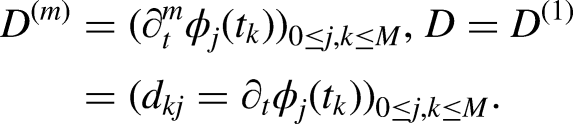
Lagrange basis polynomials in time and its differential matrix

The Legendre polynomial of degree m is (cf. Refs.^5,9)

$$L_m(t)={\displaystyle \frac{{(-1)}^m}{2^{m}m!}{\mathrm{\partial }}_t^m(1-t^2{)}^m,t\in I=(-1,1),m=0,1,2,\cdots .}$$

It is the $m-$ th eigenfunction of the singular Sturm-Liouville problem

$${\mathrm{\partial }}_t((1-t^2){\mathrm{\partial }}_{t}u(t))+\lambda u(t)=0,t\in I.$$

(2)

Related to $m-$ th eigenvalue ${\lambda }_m=m(m+1)$ . Let $t_0=-1,t_M=1$ , and $t_j(1\le j\le M-1)$ be the roots of ${\mathrm{\partial }}_t{L}_M(t)=0$ . Take $w_{M+1}(t)=(t-t_0)(t-t_1)\dots (t-t_M)$ . The Lagrange basis polynomials based on the Legendre-Gauss-Lobatto nodes $\{t_j{\}}_{j=0}^M$ are as follows:

$${\varphi }_j(t)={\displaystyle \frac{w_{M+1}(t)}{(t-t_j){\mathrm{\partial }}_t{w}_{M+1}(t_j)},j=0,1,\dots ,M,}$$

(3)

Equivalently,

$${\varphi }_j(t)={\displaystyle \frac{(t^2-1){\mathrm{\partial }}_t{L}_M(t)}{M(M+1)(t-t_j)L_M(t_j)},j=0,1,\dots ,M,}$$

(4)

Let $P_M(I)$ be the set of all polynomials of degree at most M, for $u(t)\in C(\overline{I})$ ,

$$p_M(t)=\sum _{j=0}^{N}u(t_j){\varphi }_j(t)\in P_M(I),t\in [-1,1]$$

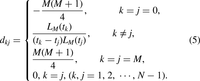
Which is the Lagrange interpolation polynomial of $u(t)$ . Calculating the $m$ -th derivative of the above equation and taking $t=t_k$ , we get that

$${\mathrm{\partial }}_t^m{p}_M(t_k)=\sum _{j=0}^{N}u(t_j){\mathrm{\partial }}_t^m{\varphi }_j(t_k).$$

Let

$$D^{(m)}=({\mathrm{\partial }}_t^m{\varphi }_j(t_k){)}_{0\le j,k\le M},D=D^{(1)}=(d_{kj}={\mathrm{\partial }}_t{\varphi }_j(t_k){)}_{0\le j,k\le M}.$$

Then $D=(d_{kj})$ is determined by (cf. Ref. ⁶ )

$$d_{kj}=\{\begin{array}{c}-{\displaystyle \frac{M(M+1)}{4},k=j=0,}\\ {\displaystyle \frac{L_M(t_k)}{(t_k-t_j)L_M(t_j)},k\ne j,}\\ {\displaystyle \frac{M(M+1)}{4},k=j=M,}\\ 0,k=j,(k,j=1,2,\cdots ,N-1).\end{array}$$

(5)

Moreover, $D^{(m)}=D^m$ (see Ref. ⁶ ).

Lagrange basis functions in velocity and its differential matrix

Let $R^{+}=(0,\mathrm{\infty })$ . The Laguerre polynomial of degree n is^15,20

$$L_n(y)={\displaystyle \frac{1}{n!}{e}^y{\mathrm{\partial }}_x^n(y^n{e}^{-y}),y\in R^{+}.}$$

It is the $n-$ th eigenfunction of the singular Sturm-Liouville problem

$${\mathrm{\partial }}_y(y{e}^{-y}{\mathrm{\partial }}_{y}u(y))+\lambda e^{-y}u(y)=0,$$

(6)

Related to $n-$ th eigenvalue ${\lambda }_n=n.$

In order to match the asymptotic behaviors of the exact solutions as $v\to +\mathrm{\infty }$ , we introduce the new interpolation function functions (cf. Refs. ^15,20). Let $\beta$ be a positive constant and

$$L_n^{(\beta )}(v)=L_n(\beta v),{\tilde{L}}_n^{(\beta )}(v)=e^{-\beta v/2}{L}_n^{(\beta )}(v),$$

Let $v_j,0\le j\le N$ be the roots of the equation: $v{\mathrm{\partial }}_v{L}_{N+1}^{(\beta )}(v)=0$ , the corresponding Lagrange basis functions are (cf. Ref. ²⁰ )

$${\phi }_j^{(\beta )}(v)={\displaystyle \frac{e^{-\beta v/2}}{\beta (N+1)e^{-\beta v_j/2}}{\displaystyle \frac{v{\mathrm{\partial }}_x{L}_{N+1}^{(\beta )}(v)}{(v_j-v)L_{N+1}^{(\beta )}(v_j)},j=0,1,2,\cdots ,N.}}$$

Let $P_N(R^{+})$ be the set of all polynomials of degree at most N, and

$${\mathcal{Q}}_{\beta ,N}(R^{+})=\{e^{-\beta v/2}\psi |\psi \in P_N(R^{+})\}.$$

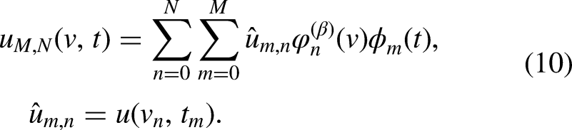
For any $u(v)\in C(\{0\}\cup R^{+})$ , the Lagrange interpolation function can be written as

$$p_N(v)=\sum _{j=0}^{N}u(v_j){\phi }_j^{(\beta )}(v)\in {\mathcal{Q}}_{\beta ,N}(R^{+}),v\in \{0\}\cup R^{+}.$$

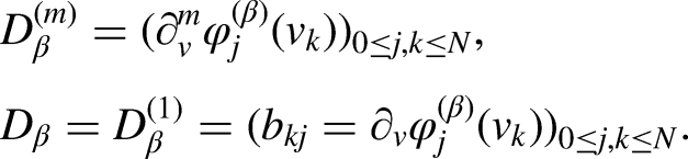
Calculating the $m$ -th derivative of the above equation and taking $v=v_k$ , we get that

$${\mathrm{\partial }}_v^m{p}_N(v_k)=\sum _{j=0}^{N}u(v_j){\mathrm{\partial }}_v^m{\phi }_j^{(\beta )}(v_k).$$

Let

$$\begin{array}{rl}& D_{\beta }^{(m)}=({\mathrm{\partial }}_v^m{\phi }_j^{(\beta )}(v_k){)}_{0\le j,k\le N},\\ & D_{\beta }=D_{\beta }^{(1)}=(b_{kj}={\mathrm{\partial }}_v{\phi }_j^{(\beta )}(v_k){)}_{0\le j,k\le N}.\end{array}$$

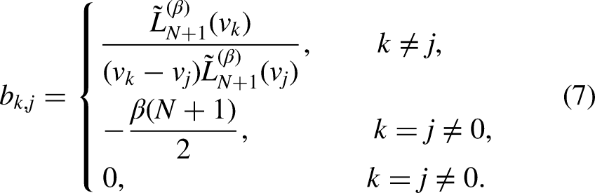
The entries of the matrix $D_{\beta }=(b_{kj}{)}_{0\le k,j\le N}$ are determined by (cf. Ref. ²⁰ )

$$b_{k,j}=\{\begin{array}{c}{\displaystyle \frac{{\tilde{L}}_{N+1}^{(\beta )}(v_k)}{(v_k-v_j){\tilde{L}}_{N+1}^{(\beta )}(v_j)},k\ne j,}\\ -{\displaystyle \frac{\beta (N+1)}{2},k=j\ne 0,}\\ 0,k=j\ne 0.\end{array}$$

(7)

Also, $D_{\beta }^{(m)}=D_{\beta }^m$ , see Ref. ⁶ Further, let, $D_{\beta }^{(2)}=({\hat{b}}_{kj}={\mathrm{\partial }}_v^2{\phi }_j^{(\beta )}(v_k){)}_{0\le j,k\le N}$ .

Spectral collocation method

To design the spectral collocation scheme, we use transformation

$$t={\displaystyle \frac{2s}{T}-1,s\in [0,T],}$$

then equation (1) is changed into

$$\{\begin{array}{c}{\displaystyle \frac{2}{T}{\mathrm{\partial }}_{t}u(v,t)={\mathrm{\partial }}_v(vu(v,t)(1+\lambda u(v,t)))+{\mathrm{\partial }}_v^{2}u(v,t),v\in (0,\mathrm{\infty }),-1<t\le 1,\lambda =\pm 1,}\\ u(v,-1)={\phi }_0(v),v\in \{0\}\cup R^{+},\\ u(0,t)={\mu }_0(t),-1\le t\le 1.\end{array}$$

(8)

Let $\mathrm{\Omega }=I\otimes R^{+},{\mathcal{Q}}_{M,N,\beta }(\mathrm{\Omega })=P_M(I)\otimes {\mathcal{Q}}_{\beta ,N}(R^{+})$ . The binary spectral collocation scheme of equation (8) is to find $u_{M,N}\in {\mathcal{Q}}_{M,N,\beta }(\mathrm{\Omega })$ , such that

$$\{\begin{array}{c}{\displaystyle \frac{2}{T}{\mathrm{\partial }}_t{u}_{M,N}(v,t)={\mathrm{\partial }}_v(v{u}_{M,N}(v,t)(1+\lambda u_{M,N}(v,t)))+{\mathrm{\partial }}_v^2{u}_{m,n}(v,t),v=v_k,t=t_l,}\\ k=1,2,\cdots ,N,l=1,2,\cdots ,M,\\ u_{M,N}(v,t_0)={\phi }_0(v),v=v_k,k=0,1,2,\cdots ,N,\\ u_{M,N}(v_0,t)={\mu }_0(t),t=t_l,l=0,1,2,\cdots ,M.\end{array}$$

(9)

The approximate solution is expanded by

$$u_{M,N}(v,t)=\sum _{n=0}^N\sum _{m=0}^M{\hat{u}}_{m,n}{\phi }_n^{(\beta )}(v){\varphi }_m(t),{\hat{u}}_{m,n}=u(v_n,t_m).$$

(10)

Then equation (9) can be written in a nonlinear system

$$\{\begin{array}{c}{\displaystyle \frac{2}{T}\sum _{n=0}^N\sum _{m=0}^M{\hat{u}}_{m,n}{\phi }_n^{(\beta )}(v_k){\mathrm{\partial }}_t{\varphi }_m(t_l)=\sum _{n=0}^N\sum _{m=0}^M{\hat{u}}_{m,n}{\phi }_n^{(\beta )}(v_k){\varphi }_m(t_l)+v_k\sum _{n=0}^N\sum _{m=0}^M{\hat{u}}_{m,n}{\mathrm{\partial }}_v{\phi }_n^{(\beta )}(v_k){\varphi }_m(t_l)}\\ +2\lambda v_k\sum _{n=0}^N\sum _{m=0}^M{\hat{u}}_{m,n}{\phi }_n^{(\beta )}(v_k){\varphi }_m(t_l)\sum _{n=0}^N\sum _{m=0}^M{\hat{u}}_{m,n}{\mathrm{\partial }}_v{\phi }_n^{(\beta )}(v_k){\varphi }_m(t_l)\\ +\lambda (\sum _{n=0}^N\sum _{m=0}^M{\hat{u}}_{m,n}{\phi }_n^{(\beta )}(v_k){\varphi }_m(t_l){)}^2+\sum _{n=0}^N\sum _{m=0}^M{\hat{u}}_{m,n}{\mathrm{\partial }}_v^2{\phi }_n^{(\beta )}(v_k){\varphi }_m(t_l),\\ k=1,2,\cdots ,N,l=1,2,\cdots ,M,\\ \sum _{n=0}^N\sum _{m=0}^M{\hat{u}}_{m,n}{\phi }_n^{(\beta )}(v_k){\varphi }_m(t_0)=\phi (v_k),k=0,1,2\dots N,\\ \sum _{n=0}^N\sum _{m=0}^M{\hat{u}}_{m,n}{\phi }_n^{(\beta )}(0){\varphi }_m(t_l)=\mu (t_l),l=0,1,2\dots M.\end{array}$$

By using equations (5) and (7), the above formulation is

$$\{\begin{array}{c}{\displaystyle \frac{2}{T}\sum _{m=0}^M{\hat{u}}_{m,k}{\hat{d}}_{l,m}={\hat{u}}_{l,k}+v_k\sum _{n=0}^N{\hat{u}}_{l,n}{b}_{k,n}+\lambda {\hat{u}}_{l,k}^2+2\lambda v_k{\hat{u}}_{l,k}\sum _{n=0}^N{\hat{u}}_{l,n}{b}_{k,n}+\sum _{n=0}^N{\hat{u}}_{l,n}{\hat{b}}_{k,n},}\\ l=1,2,\dots M,k=1,2,\dots N,\\ {\hat{u}}_{0,k}=\phi (v_k),k=0,1,2\dots N,\\ {\hat{u}}_{l,0}=\mu (t_l),l=0,1,2\dots M.\end{array}$$

(11)

equivalently

$$\{\begin{array}{c}{\displaystyle \frac{2}{T}({\hat{u}}_{1,k}{\hat{d}}_{l,1}+{\hat{u}}_{2,k}{\hat{d}}_{l,2}\dots +{\hat{u}}_{M,k}{\hat{d}}_{l,M})={\hat{u}}_{l,k}+v_k({\hat{u}}_{l,1}{b}_{k,1}+{\hat{u}}_{l,2}{b}_{k,2}\dots +{\hat{u}}_{l,N}{b}_{k,N})+\lambda {\hat{u}}_{l,k}^2}\\ +2\lambda v_k{\hat{u}}_{l,k}({\hat{u}}_{l,1}{b}_{k,1}+{\hat{u}}_{l,2}{b}_{k,2}\dots +{\hat{u}}_{l,N}{b}_{k,N})+({\hat{u}}_{l,1}{\hat{b}}_{k,1}+{\hat{u}}_{l,2}{\hat{b}}_{k,2}\dots +{\hat{u}}_{l,N}{\hat{b}}_{k,N})\\ -{\displaystyle \frac{2}{T}{\hat{u}}_{0,k}{\hat{d}}_{l,0}+v_k{\hat{u}}_{l,0}{b}_{k,0}+2\lambda v_k{\hat{u}}_{l,k}{\hat{u}}_{l,0}{b}_{k,0}+{\hat{u}}_{l,0}{\hat{b}}_{k,0}}\\ k=1,2\dots N,l=1,2,\dots M.\end{array}$$

(12)

Expand the above equation with respect to k and l, and obtain its matrix form as,

$$\begin{array}{rl}{\displaystyle \frac{2}{T}DX}& =X+X{B}^{T}F+\lambda (X.*X)+2\lambda X.*(X{B}^{T}F)\\ & +X{C}^T-{\displaystyle \frac{2}{T}G+HF+2\lambda X.*(HF)+V,}\end{array}$$

(13)

with

$$\begin{array}{rl}& X=\left(\begin{array}{cccc}{\hat{u}}_{1,1}& {\hat{u}}_{1,2}& \cdots & {\hat{u}}_{1,N}\\ {\hat{u}}_{2,1}& {\hat{u}}_{2,2}& \cdots & {\hat{u}}_{2,N}\\ ⋮& ⋮& \ddots & ⋮\\ {\hat{u}}_{M,1}& {\hat{u}}_{M,2}& \cdots & {\hat{u}}_{M,N}\end{array}\right),\\ & D=\left(\begin{array}{cccc}{\hat{d}}_{1,1}& {\hat{d}}_{1,2}& \cdots & {\hat{d}}_{1,M}\\ {\hat{d}}_{2,1}& {\hat{d}}_{2,2}& \cdots & {\hat{d}}_{2,M}\\ ⋮& ⋮& \ddots & ⋮\\ {\hat{d}}_{M,1}& {\hat{d}}_{M,2}& \cdots & {\hat{d}}_{M,M}\end{array}\right),\\ & B=\left(\begin{array}{cccc}{b}_{1,1}& b_{1,2}& \cdots & b_{1,N}\\ b_{2,1}& b_{2,2}& \cdots & b_{2,N}\\ ⋮& ⋮& \ddots & ⋮\\ b_{N,1}& b_{N,2}& \cdots & b_{N,N}\end{array}\right),\end{array}$$

$$\begin{array}{rl}& C=\left(\begin{array}{cccc}{\hat{b}}_{1,1}& {\hat{b}}_{1,2}& \cdots & {\hat{b}}_{1,N}\\ {\hat{b}}_{2,1}& {\hat{b}}_{2,2}& \cdots & {\hat{b}}_{2,N}\\ ⋮& ⋮& \ddots & ⋮\\ {\hat{b}}_{N,1}& {\hat{b}}_{N,2}& \cdots & {\hat{b}}_{N,N}\end{array}\right),\\ & G=\left(\begin{array}{c}{\hat{d}}_{1,0}\\ {\hat{d}}_{2,0}\\ ⋮\\ {\hat{d}}_{M,0}\end{array}\right)({\hat{u}}_{0,1},{\hat{u}}_{0,2},\cdots ,{\hat{u}}_{0,N}),\\ & F=\left(\begin{array}{c}{v}_{1}0\cdots 0\\ 0v_2\cdots 0\\ ⋮\cdots \\ 00\cdots v_N\end{array}\right),\end{array}$$

$$\begin{array}{rl}& H=\left(\begin{array}{c}{\hat{u}}_{1,0}\\ {\hat{u}}_{2,0}\\ \dots \\ {\hat{u}}_{M,0}\end{array}\right)(b_{1,0},b_{2,0},\dots ,b_{N,0}),\\ & V=\left(\begin{array}{c}{\hat{u}}_{1,0}\\ {\hat{u}}_{2,0}\\ \dots \\ {\hat{u}}_{M,0}\end{array}\right)({\hat{b}}_{1,0},{\hat{b}}_{2,0},\dots ,{\hat{b}}_{N,0}),\end{array}$$

where $".*"$ defined as the product of the corresponding elements of two matrices of the same order.

Numerical result

We convert equation (13) into a nonlinear system. To do this, let

$$\begin{array}{rl}Y=& ({\hat{u}}_{1,1}{\hat{u}}_{1,2}\cdots {\hat{u}}_{1,N},{\hat{u}}_{2,1}{\hat{u}}_{2,2}\cdots {\hat{u}}_{2,N},\cdots ,{\hat{u}}_{M,1}\\ & {\hat{u}}_{M,2}\cdots {\hat{u}}_{M,N}),\\ R1=& ({\hat{d}}_{1,0}({\hat{u}}_{0,1},{\hat{u}}_{0,2},\cdots ,{\hat{u}}_{0,N}),{\hat{d}}_{2,0}({\hat{u}}_{0,1},{\hat{u}}_{0,2},\cdots ,{\hat{u}}_{0,N}),\\ & \cdots ,{\hat{d}}_{M,0}({\hat{u}}_{0,1},{\hat{u}}_{0,2},\cdots ,{\hat{u}}_{0,N})),\\ R2=& ({\hat{u}}_{1,0}(v_1{b}_{1,0},v_2{b}_{2,0},\dots ,v_N{b}_{N,0}),{\hat{u}}_{2,0}(v_1{b}_{1,0},v_2{b}_{2,0},\\ & \dots ,v_N{b}_{N,0}),\dots ,{\hat{u}}_{M,0}(v_1{b}_{1,0},v_2{b}_{2,0},\dots ,v_N{b}_{N,0})),\\ R3=& ({\hat{u}}_{1,0}({\hat{b}}_{1,0},{\hat{b}}_{2,0},\dots ,{\hat{b}}_{N,0}),{\hat{u}}_{2,0}({\hat{b}}_{1,0},{\hat{b}}_{2,0},\dots ,{\hat{b}}_{N,0}),\\ & \dots ,{\hat{u}}_{M,0}({\hat{b}}_{1,0},{\hat{b}}_{2,0},\dots ,{\hat{b}}_{N,0})).\end{array}$$

Then equation (13) can be written as

$$\begin{array}{rl}& \left({\displaystyle \frac{2}{T}D\otimes E_N-E_M\otimes E_N-E_M\otimes C}\right)Y=(E_M\otimes (F*B))Y\\ & +\gamma (Y.*Y)+2\gamma Y.*((E_M\otimes (F*B))Y)-{\displaystyle \frac{2}{T}R1+R2}\\ & +2\gamma *Y.*R2+R3,\end{array}$$

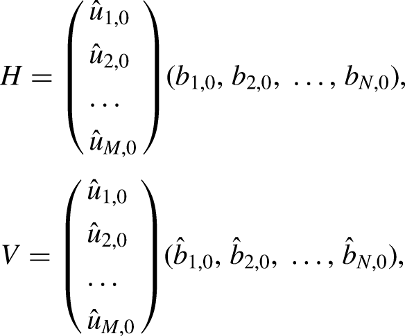
where $"E_n"$ stands for n order identity matrix, $"\otimes "$ means the times of Kronecker. Let

$$\begin{array}{rl}F(Y)=& \left({\displaystyle \frac{2}{T}D\otimes E_N-E_M\otimes E_N-E_M\otimes C}\right)Y\\ & -(E_M\otimes (F*B))Y-\lambda (Y.*Y)-2\lambda Y.\\ & *((E_M\otimes (FB))Y)+{\displaystyle \frac{2}{T}R1-R2-2\lambda Y.*R2-R3,}\end{array}$$

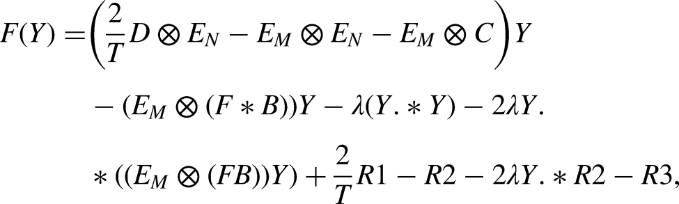
the Jacobi matrix of Newton iteration is as follows:

$$\begin{array}{rl}J(Y)=& \left({\displaystyle \frac{2}{T}D\otimes E_N-E_M\otimes E_N-E_M\otimes C}\right)\\ & -(E_M\otimes (FB))-2\lambda diag(Y)\\ & -2\lambda [diag((E_M\otimes (FB))Y)+diag(Y)(E_M\otimes (FB))]\\ & -2\lambda diag(R2),\end{array}$$

Where $diag(Y)$ represents a diagonal matrix generated by the elements of vector Y. The Newton iteration scheme is as follows:

$$Y_{n+1}=Y_n-(J(Y_n){)}^{-1}F(Y_n),n=0,1,2,\cdots .$$

(14)

In actual computation, we take

$$Y_0={\left(\begin{array}{cc}{\phi }_0(v_1){\phi }_0(v_2)\cdots {\phi }_0(v_N)& {\phi }_0(v_1){\phi }_0(v_2)\cdots {\phi }_0(v_N)\cdots \\ & {\phi }_0(v_1){\phi }_0(v_2)\cdots {\phi }_0(v_N)\end{array}\right)}^T.$$

and the end condition of iteration: $\mathrm{\forall }\epsilon >0,\Vert X_{n+1}-X_n{\Vert }_{\mathrm{\infty }}<\epsilon .$

We choose an appropriate right term $f(v,t)$ in equation (1) with $\lambda =1$ so that equation (1) has the following exact solution (cf. Ref. ¹³ )

$$U(v,s)={\displaystyle \frac{4}{\sqrt{s+1}}\tanh \left({\displaystyle \frac{\sqrt{6}}{12}\left(v-{\displaystyle \frac{5\sqrt{6}}{6}s}\right)}\right)e^{-\frac{1}{2}{(\sigma v)}^2},v>0,0<s\le T,}$$

(15)

with initial value conditions and boundary conditions ( $\sigma$ is a positive constant)

$${\phi }_0(v)=4\tanh {\displaystyle \frac{\sqrt{6}}{12}(v)e^{-\frac{1}{2}{(\sigma v)}^2},{\mu }_0(s)={\displaystyle \frac{4}{\sqrt{s+1}}\tanh {\displaystyle \frac{\sqrt{6}}{12}\left(-{\displaystyle \frac{5\sqrt{6}}{6}s}\right).}}}$$

We use the maximum error below to measure numerical error

$$E_{M,N}=\underset{1\le l\le M,1\le k\le N}{max}|u_{M,N}(v_k,t_l)-U(v_k,t_l)|.$$

In Figure 1, the errors ${\log }_{10}{E}_{M,N}$ versus N of the scheme (13) with $M=30,T=1$ , $\sigma =1$ in (15) and different $\beta$ in (10) is plotted. Clearly, the error rapidly decreases with the increase of N and indicates spectral accuracy in the velocity direction. Additionally, by appropriately selecting the value of the proportional factor $\beta$ in the basis function, the error accuracy can be improved. However, how to choose the value of $\beta$ is an open problem.

Figure 1.

${\log }_{10}{E}_{M,N}$ versus N of (14) with $\sigma =1,$ and different $\beta .$

In Figure 2, the errors ${\log }_{10}{E}_{M,N}$ versus N of the scheme (13) with $M=17,T=1,$ $\sigma =0.35$ in (15) and $\beta =2$ in (10) is drawn. It indicates that scheme (13) is still effective for solutions with slower decay. When the parameter $\sigma <1$ in (15), the decay of the function $U(v,s)$ is relatively slow as $v\to +\mathrm{\infty }$ . By appropriately increasing the degree of the velocity direction polynomial, higher accuracy can be achieved.

Figure 2.

${\log }_{10}{E}_{M,N}$ versus N of (14) with $\sigma =0.35,$ and $\beta =2.$

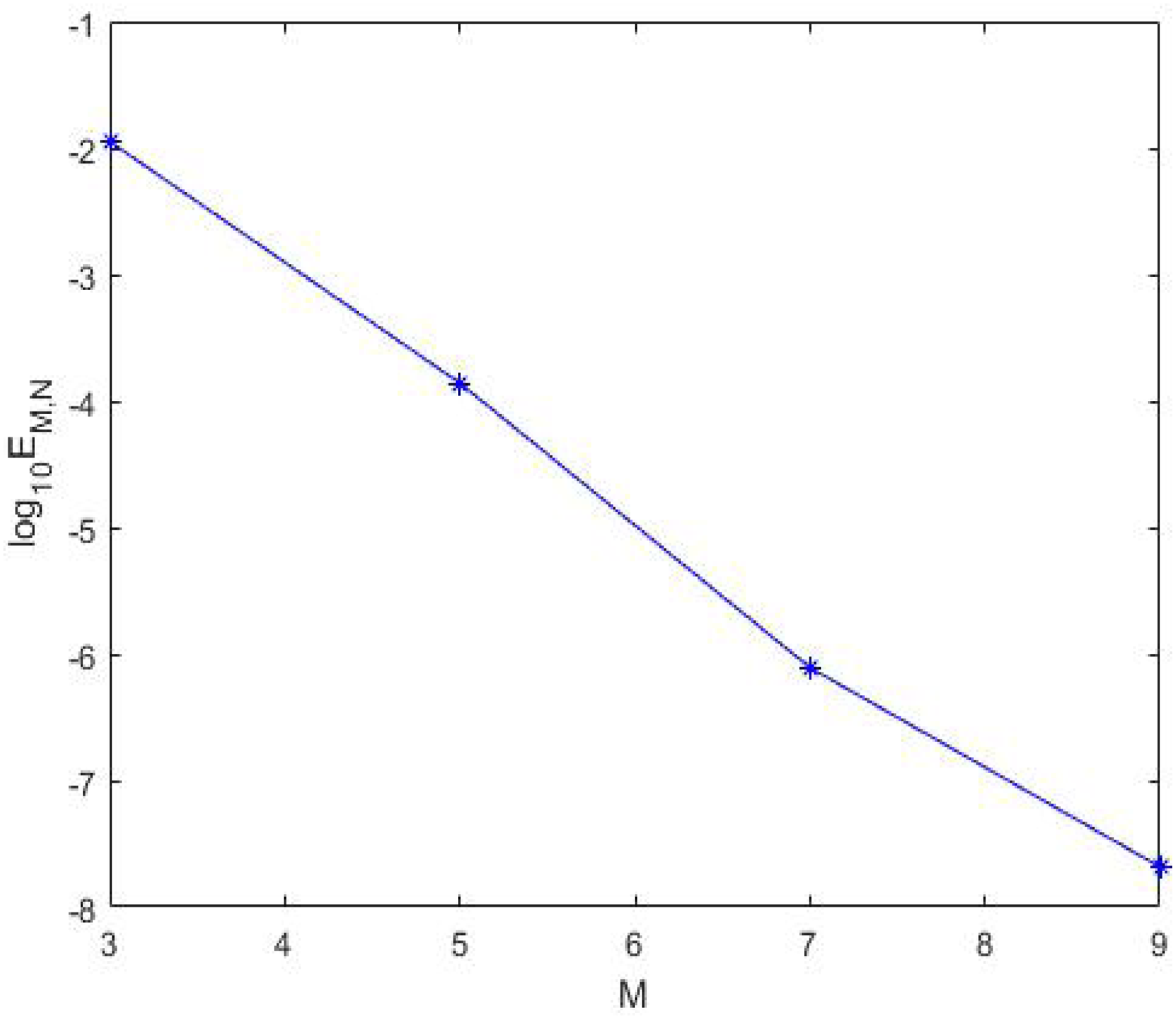
In Figure 3, the errors ${\log }_{10}{E}_{M,N}$ versus M of the scheme (13) with $N=70,T=1$ , $\sigma =1$ in (15) and $\beta =3$ in (10) is depicted. It indicates that the algorithm can also achieve spectral accuracy in the time direction.

Figure 3.

${\log }_{10}{E}_{M,N}$ versus M of (13) with $\beta =3,\sigma =1,N=70.$

In Figure 4, the errors ${\log }_{10}{E}_{M,N}$ versus N of the scheme (13) with $M=60$ , $T=20$ , $\sigma =1$ in (15) and $\beta =4$ in (10) is presented. It indicates that the algorithm can also achieve spectral accuracy for a long time.

Figure 4.

${\log }_{10}{E}_{M,N}$ versus N of (13) with $\beta =4,\sigma =1,M=60.$

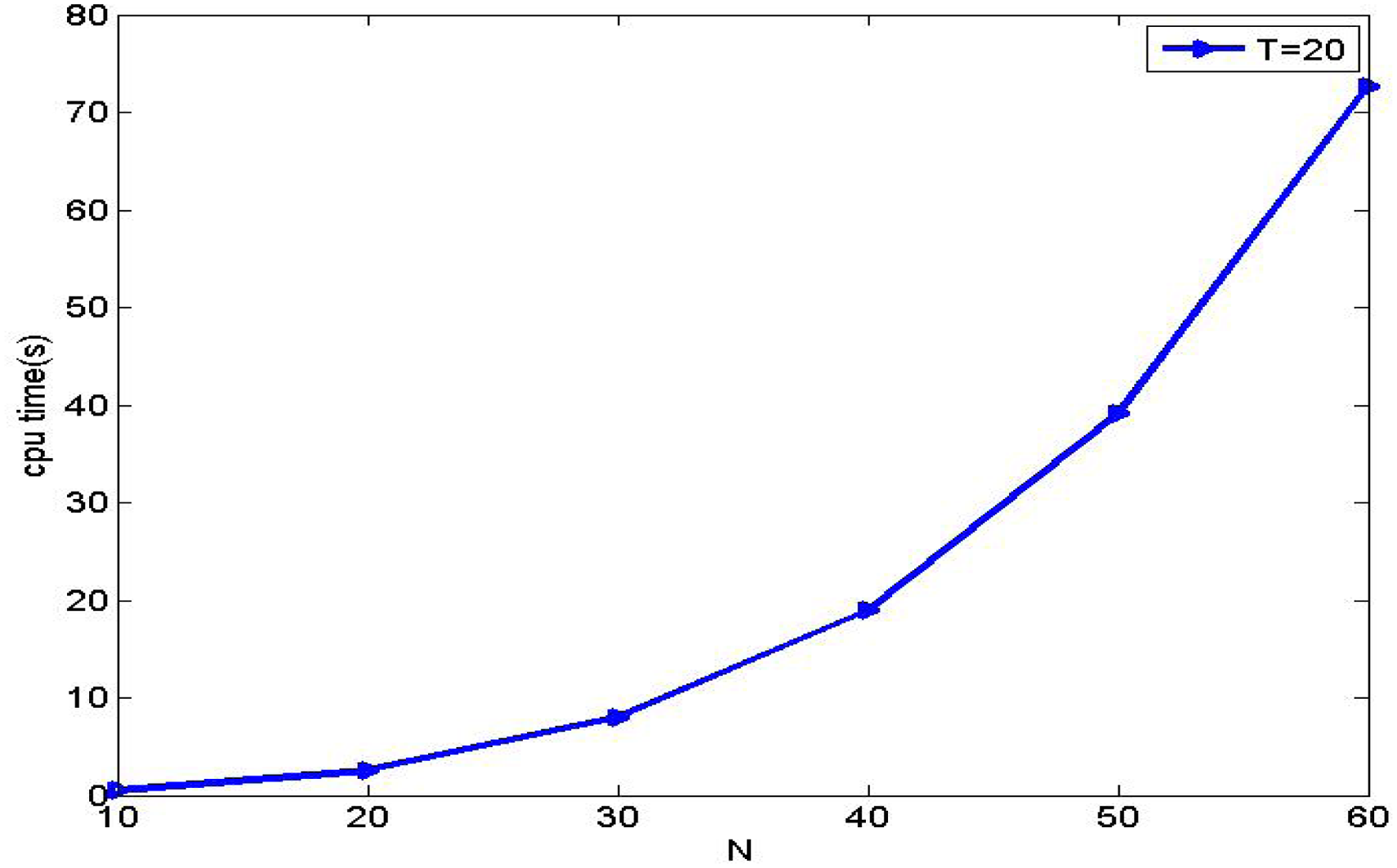
In Figure 5, the CPU time(s) versus N of the scheme (13) with $M=60,T=20$ , $\sigma =1$ in (15), $\beta =4$ in (10), with a CPU consumption of only over 70 s and T = 20, is given, which indicates that the algorithm proposed in this article is efficient.

Figure 5.

Cputime(s) versus N of (13) with $\beta =4,\sigma =1,M=60.$

Compared to references,^13–15 it is noteworthy that the suggested algorithm balances the number of nodes used for discretizing the time direction utilizing the difference method with the polynomial degree in the velocity direction implementing the spectral method. Furthermore, there is a suitable proportion of polynomial degrees in both the time and velocity direction. This results in a reduction in the overall number of nodes, making this method advantageous.

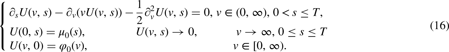
Next, let's consider the following linear homogeneous equation (cf. Ref. ²¹ ):

$$\{\begin{array}{c}{\mathrm{\partial }}_{s}U(v,s)-{\mathrm{\partial }}_v(vU(v,s))-{\displaystyle \frac{1}{2}{\mathrm{\partial }}_v^{2}U(v,s)=0,v\in (0,\mathrm{\infty }),0<s\le T,}\\ U(0,s)={\mu }_0(s),U(v,s)\to 0,v\to \mathrm{\infty },0\le s\le T\\ U(v,0)={\phi }_0(v),v\in [0,\mathrm{\infty }).\end{array}$$

(16)

We expand the numerical solution $u_{M,N}(v,t)$ of equation (16) like equation (10), like equation (13), the algorithm scheme of equation (16) is as follows:

$${\displaystyle \frac{2}{T}DX-X-X{B}^{T}F-{\displaystyle \frac{1}{2}X{C}^T=-{\displaystyle \frac{2}{T}G+HF+{\displaystyle \frac{1}{2}V.}}}}$$

(17)

There exists exact solution of equation (16),

$$U(v,s)=2(2v^2-1)e^{-(v^2+2s)},v>0,0<s\le T.$$

(18)

In Figure 6, the errors ${\log }_{10}{E}_{M,N}$ versus N of the scheme (17) with $M=10,T=1,$ and $\beta =3$ in (10) is drawn. It indicates that scheme (17) is effective for solutions of (16) with a homogeneous term $f(v,s)\equiv 0$ at its right side.

Figure 6.

${\log }_{10}{E}_{M,N}$ versus N of (16) with $\beta =3,M=10.$

In Figure 7, the errors ${\log }_{10}{E}_{M,N}$ versus M of the scheme (17) with $N=80,T=1,$ and $\beta =3$ in (10) is depicted. It indicates that the algorithm can also achieve spectral accuracy in the time direction for a homogeneous term $f(v,s)\equiv 0$ at its right side.

Figure 7.

${\log }_{10}{E}_{M,N}$ versus M of (16) with $\beta =3,N=80.$

It should be pointed out that for the nonlinear homogeneous Fokker Planck equation (1), finding its exact solution is an open problem. Here, we only consider the binary spectral collocation method for a linear homogeneous Fokker Planck equation (16). In the future, we will report the relevant results of the binary spectral collocation method for the nonlinear homogeneous Fokker Planck equation (1).

Conclusions

In this paper, Legendre Gauss Lobatto node and Laguerre Gauss Radau node are used as collocation points in the time direction and velocity direction respectively. Legendre polynomial and Laguerre polynomial are used to construct the problem of binary Lagrange interpolation polynomial solving the nonlinear and linear Fokker Planck equation, which is time–velocity discretization into a nonlinear matrix equation, then it is solved by changing into nonlinear and linear system respectively. Numerical experiments show that the approximate solution can better approximate the theoretical solution, and the algorithm scheme has spectral accuracy in the time direction and velocity direction respectively. Combined with orthogonal polynomials interpolation technology, the difference error is fundamentally reduced and the accuracy of numerical calculation is improved. Numerical experiments show that the algorithm has a high accuracy for calculating partial differential equations with variable coefficient terms. The algorithm has strong flexibility, and can be optimized by adjusting parameters, as shown in Figure 1; better results can be achieved by changing the value of the scaling factor. The algorithm can also solve other nonlinear or linear problems.