Sage Journals: Discover world-class research

Abstract

The real world is nonlinear and in the control application field, this aspect needs to be resolved to build models so we need to refer to nonlinear system modeling techniques. Neuro-fuzzy systems and modular neural networks (NNs) are among the best modeling approaches for nonlinear systems. The combined features of both approaches provide better models. Thus, we propose in this paper a neuro-fuzzy modular architecture for modeling nonlinear systems. The modular architecture consists of dividing a nonlinear problem into several simpler subproblems. We assigned to each subproblem an NN. Each NN provides individual solutions that will be combined to provide a general solution to the original problem. In this respect, the decomposition of the original problem is based on a fuzzy decision mechanism. This mechanism consists of a set of fuzzy rules for processing nonlinear problems using two different strategies. The first involves training only the network weights, and the second adds the fuzzy set parameters to the training step. A comparative study of both strategies reveals the competence of the second strategy in providing better accuracy and simplicity. Using the neuro-fuzzy combination among the modular NNs reduces the complexity of the original problem and achieves much better performance. The proposed architecture is evaluated by two second-order nonlinear systems, a numerical system and a real system called “the chemical reactor,” which is used to carry out a chemical reaction not only in chemical and biochemical engineering, but also in the petrochemical industry. For both systems, the proposed approach provides better performance in terms of the learning time, learning error, and number of neurons.

Keywords

Modeling nonlinear systems neuro-fuzzy systems modular neural networks complex problem fuzzy rules the chemical reactor.

Introduction

Nonlinear behavior appears in many engineering problems such as electrical, mechanical, chemical problems, and even physics¹ and health issues.^2,3,4 The challenge in modeling nonlinear systems is to ensure an effective and accurate model for control requirements.^5,6 Many tools have been used to solve nonlinear problems in modeling namely fuzzy systems (FSs), multi-model systems (MMSs), and artificial neural networks (ANNs).

FSs have been efficient in modeling complex nonlinear systems using linear local models.^7,8 Indeed, among the existing FSs, Takagi–Sugeno (TS) is the most used.^9–11 The TS model suggested a fuzzy process based on a set of fuzzy rules. Each rule defined a local linear model. Local models are easily connected by fuzzy membership functions to describe a global nonlinear system.^12,13 Researchers have frequently used FS in many decision-making problems of real-life situations.^14,15

The MMSs are a powerful tool to resolve the problem of modeling complex nonlinear systems.^16,17 The complex problem is divided into a set of subproblems, each of which makes a local model (generally linear), and each model describes the problem in a specific operating zone. It can be considered as an expert in its domain, and the individual network is trained only in this domain. The contribution rate of each local model, called the activation degree, must first be determined, and then the combination of all local models allows us to obtain the global model.

ANNs are computing systems with interconnected nodes. Each node represents a perceptron. The perceptron feeds the input signal into an activation function that usually is nonlinear. Using algorithms, ANNs have a high capability to recognize hidden patterns and correlations in raw data, and continuously learn and improve over time in order to solve complex problems of real-time situations and then they lead to an effective visual analysis.

Many researchers have successfully demonstrated that ANNs are promising tools for solving nonlinear problems. Thus, systems based on ANN can model highly nonlinear processes^18–20 and they are able to approximate both deterministic and stochastic processes.^21–23

Owing to the interesting features of ANN,^24–26 such as learning and generalization ability, approximation, robustness, and simplicity, the research in the field of ANN has rapidly grown, and their field of application is widely extended. Indeed, ANNs are often used in many control structures and can be applied in various engineering domains.^27,28

Most systems employ monolithic networks to solve a specific task. However, if the system has a large amount of data, a high input dimension, or important nonlinearities, it is unlikely and sometimes impossible to establish a good architecture for a single network that can solve the problem. Therefore, a large and complex ANN is required. However, large networks are often difficult to train and cannot achieve the desired performance.

In order to overcome the deficiencies of monolithic neural networks (NNs), many approaches have been proposed.

Modular NNs (MNNs) are among the most powerful techniques for solving nonlinear problems. The concept of modularity involves subdividing complex tasks into simpler subtasks. The nonlinear problem is composed of a hierarchy of networks, each of which performs a simpler single module. A module is smaller than a monolithic network.^29,30 MNNs adopt different techniques for learning. Most of them are based on the “divide-and-conquer strategy.” Thus, it is easier to train a single module. Modules are trained independently or simultaneously and then combined in some way.

ANNs are very effective for problems with enough training data, FSs are popular computing frameworks based on the concept of fuzzy set theory. Therefore, ANN and FS, as two important techniques of artificial intelligence, have been developed and improved for years to be up to date with technological progress. The fusion of these two techniques forms a neuro-fuzzy system (NFS). Each of these techniques has its own advantages and disadvantages. However, when mixed, they provided better results. Therefore, NNs introduce their computational characteristics of learning in fuzzy systems and receive from them the interpretation and clarity of system representation.³¹

Thanks to the combined features of both techniques, NFSs are useful when solving nonlinear problems.^32–34

To this end, in this paper, we will use all these tools in one architecture called the neuro-fuzzy modular system (NFMS) for nonlinear system modeling.

The key contributions and objectives of the proposed approach are:

We will combine the ANNs with FSs by using the most relevant properties of each technique.

By decomposing the original problem into several simple subproblems, the neuro-fuzzy approach adopts a modular structure that can represent the complex problem more efficiently.

The learning procedure includes the learning of fuzzy parameters within the NN's parameters.

Learning the NFMS networks is simpler than learning the whole network in terms of convergence time and precision.

The NFMS will be detailed in the “The neuro-fuzzy modular system” section, after the related works section. It employs two approaches: local and global approaches. In the classic design, only the weights of NNs are updated. However, in the global model, all parameters (weights of NNs and fuzzy rule parameters) were considered for training.

To demonstrate the effectiveness of the proposed method, simulation examples are provided in the “Nonlinear dynamic system using the ‘NFMS’” section. After comparing the two approaches, the concluding remarks are presented in the final section.

Related works

Modular neural networks

MNNs contain several NNs that work independently and do not interact with each other during learning. Each network performs only a particular part of the overall bigger task, and all the networks are required to achieve the complete task. This task is performed using a special module called an integrator³⁵ (as shown in Figure 1).

Figure 1.

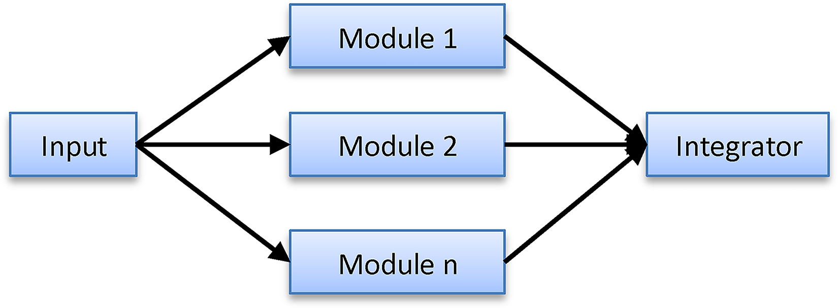
Schematic of a modular neural network.

This concept allows complex computing processes to be done more efficiently.

They are built to surpass the performance improvement caused by task decomposition.

Several advantages of modularity, such as reducing model complexity, combining techniques, learning different tasks simultaneously, and providing robustness, have led to the development of modular systems.²⁹

To conceive an MNN, it is fundamental to achieve the following three steps^36–38:

The decomposition of the task into several subtasks, and the assignment of each subtask to one module of the MNN in order to define the number and the structure of local models.

The organization of the modular structure (training modules): modules would learn in parallel or in a certain sequence according to the design.

Module combination strategy: When the entire network is ready to operate, a multimodule decision-making strategy must be adopted. This strategy enables the grouping of different local decisions in one module by interpolation skills of the local models. This is called communication between the models.

There is a variety of MNNs, they can be classified according to:

Task decomposition: There are two methods for task decomposition: explicit decomposition (prior knowledge)^39–41 and automatic decomposition.^38,42 Class decomposition is also used to deal with classification problems.

Training modules: The learning procedure of each subproblem can be independent,⁴³ sequential,⁴⁴ cooperative,⁴⁵ and incremental.⁴⁶

Module combination strategy: The relationship between modules may vary from complete decoupling through cooperation to competition.³⁸

The main domains of application of MNN are forecasting,^47,48 classification,^49,50 signal and image processing,⁵¹ control,^17,29 and modeling.^52,53

Neuro-fuzzy systems

Most combinations of techniques based on NNs and FSs are called NFSs. The first research on the NFS dates back to the early 1990s.

There are several approaches to combine ANN and FS according to the application. Different combinations of these techniques can be classified into three categories.^54–57

Cooperative NFS⁵⁸: A cooperative model can be considered as a pre-processor, where the ANN learning mechanism determines the FS membership functions or fuzzy rules from the training data. Once the FS parameters are determined, ANN is removed, and only the fuzzy system is executed (Figure 2).

Concurrent NFS⁵⁹: In concurrent systems, the NN and fuzzy system work continuously together. In general, the NN preprocesses the inputs of the fuzzy system, or vice versa (Figure 3).

Hybrid NFS^31,56: In this category, an NN is used to learn some parameters of the fuzzy system (parameters of the fuzzy sets, fuzzy rules, and weights of the rules) in an iterative manner. There are several methods to develop hybrid models. Although these models have similar backgrounds, they have basic differences.

Figure 2.

Cooperative neuro-fuzzy system.

Figure 3.

Concurrent neuro-fuzzy system.

In cooperative and concurrent NFSs, the results are not fully interpretable, which is a disadvantage. However, in hybrid NFSs, learning through examples and easy interpretation of results is attained.

Many researchers have used the neuro-fuzzy term to refer only to a hybrid NFS. The most well-known neuro-fuzzy architectures are^31,56,59:

Fuzzy adaptive learning control network.⁶⁰

Neuro-fuzzy networks with local linear models.⁶¹

Adaptive fuzzy inference system.⁶²

Neuro-fuzzy expert system (SENFpHCTRL).³²

Generalized approximate reasoning-based intelligent control.⁶³

Neuro-fuzzy control.⁵⁶

Fuzzy inference environment software with tuning.⁶⁴

Fuzzy Net.⁶⁵

Self-constructing neural fuzzy inference network.⁶⁶

Dynamic/evolving fuzzy NNs.⁶⁷

In the following section, we will introduce our approach to modeling nonlinear systems using the NFMS. The structure of the proposed NFMS has been studied in previous studies.^68,69 It is composed of a fuzzy system with a set of NNs as the conclusions of fuzzy rules. The entire system constitutes a powerful modeling tool for complex systems. In Turki et al.,⁶⁸ a local learning algorithm has been used for the training of the NFMS. Then, in Turki and Chtourou,⁶⁹ the training of the NNs was accomplished by an overall algorithm in which all the NNs were treated simultaneously. In this study, all parameters defining the NFMS structure were considered in the training step. In other words, the membership function parameters and synaptic weights of all the NNs were adjusted by the proposed algorithm.

The neuro-fuzzy modular system

General description and architecture

The multilayer perceptron (MLP) is mainly used for modeling nonlinear systems having significant degrees of complexity.⁷⁰ As the MLP is a supervised network, the input neurons are intended to gather information that is transformed by the hidden neurons into the output ones. Each input neuron is connected to all neurons in the next layer by connections whose weights are arbitrary. A neuron in the hidden or output layer combines its inputs into a single value that is transmitted to the outputs.

NNs are universal approximators, characterized by their ability to acquire knowledge through examples. Thus, any complex problem can be solved using a single NN. According to several studies,^28,70 an MLP with one layer of hidden neurons is a universal approximator. All the NNs that will be studied in this study have one hidden layer architecture.

The structure of the MLP can be described as shown in Figure 4.

Figure 4.

Structure of an MLP.

The training of an MLP is usually an iterative process in which the network weights are adjusted at each iteration according to a training algorithm before reaching their final values.⁶⁹

The learning procedure requires:

Training set composed of a given number of examples. This consists of a vector that can be applied to the network input. This training set should be sufficiently rich to cover the possible area of operation of the network.

Cost function that measures the performance of a neural model.

A training algorithm for minimizing cost function.

Generally, training requires a relatively long period and includes four calculation steps.

Initialization of synaptic weights of the network.

Presentation of the input vector and propagation of states.

Computation of the error at the output of the network.

Computation of the vector of weight corrections.

For this type of network, the backpropagation algorithm is the most commonly used learning algorithm. For each example presented to the network, the estimated output was calculated by propagating the computation from one layer to another until the output layer. In addition, an error can be calculated and backpropagated in the network to adjust each weight. This sequence was repeated until the error converged to nearly zero.

The sigmoid function is used as an activation one:

f (z) = \frac{1}{1 + e^{- z}}

(1)

The derivative of this function is:

f^{'} (z) = f (z) [1 - f (z)]

(2)

The cost function is given by:

E^{p} = \frac{1}{2} [y^{p} (k + 1) - y_{m}^{p} (k + 1)]^{2}

(3)

y^{p} (k + 1)

and

y_{m}^{p} (k + 1)

represent, respectively, the system and the model outputs of the example p.

Despite the universal approximation property, the complexity of some problems can make them difficult to solve by using a simple single NN. Therefore, we propose a solution to reduce the complexity of a problem by dividing it into simpler subproblems.

The proposed approach uses an NFMS architecture. The NFMS can be considered as a TS fuzzy system where each rule has an MLP as a conclusion (Figure 5).

Figure 5.

The neuro-fuzzy modular system.

The main idea of this approach is based on the decomposition of a system into several subsystems to build local NNs. For decomposition, we use the TS fuzzy system based on fuzzy rules. Therefore, each rule represents a local NN (LNN), and the system output is obtained by interpolation between them.

Commonly used, the TS fuzzy models propose an inference scheme in which the conclusion of a fuzzy rule is a weighted linear combination of crisp inputs. By contrast, in this study, we consider a nonlinear system (an NN) as a conclusion for each fuzzy rule. Therefore, the nonlinear behavior of the learning set is subdivided into other sets with petty nonlinearities owing to the small domain of the subsets.

We associate a single NN with one hidden layer and an appropriate number of hidden neurons in each subsystem.

Mathematically, this complex behavior is described by a variable x(k), called the input variable. We divided the operating space of the system into h zones, each corresponding to a local domain. Then, we define i (i = 1, 2,…, h) functions representing these local domains and describe the system behavior in these areas. The behavior of the global system is obtained by associating h local domains.

The validity degree of a local domain is determined by an activation function $μ_{i}$ that depends on variable x(k). The number of local domains was chosen arbitrarily, considering the richness of the principal domain. The larger the principal domain, the more local the domains.

The input variable domain D represents the union of local domains:

D = \cap_{i} D^{i}

The fuzzy decision mechanism is based on a set of fuzzy rules, where each network is described by a local fuzzy rule function.⁶⁸

\begin{matrix} R_{i} : If x_{1} (k) i s A_{i}^{1} and \dots and x_{j} (k) i s A_{i}^{j} \\ and \dots then y_{m}^{i} (k + 1) = F_{i} (x (k)) \end{matrix}

(4)

A_{i}^{j}

are fuzzy sets characterized by a Gaussian membership function centered at

c_{i}^{j}

(j = 1,…, n).

$F_{i}$ is an MLP with one hidden layer and one output.

LNNs will be combined by a fuzzy inference system to compute the NFMS output.

If $y_{m}^{i} (k + 1)$ represents the output of the ith local model, then the output of the NFMS is computed as follows:

y_{m} (k + 1) = \frac{\sum_{i = 1} μ_{i} y_{m}^{i} (k + 1)}{\sum_{i} μ_{i}}

(5)

The validity degree of the ith fuzzy rule, μ_i, is given by:

μ_{i} = \prod_{j = 1}^{n} μ_{j i}

(6)

When a Gaussian function is used, the activation degree, μ_ji, is given by:

μ_{j i} = \exp [\frac{- {(x_{j} - c_{j i})}^{2}}{2 σ_{j}^{2}}]

(7)

c_i and σ _i represent, respectively, the centers and the openings of the Gaussian functions.

In this approach, the learning concept has to do with all local networks simultaneously,⁶⁹ that is, for each input introduced to the network, we calculate the validity degree μ_i of each local behavior, and then automatically adjust the parameters of different networks during the learning phase.

Training algorithm

For the architecture described above, two synthetic approaches are possible: partial and global.

In the partial model, only the weights are changed during learning. In the global model, fuzzy rule parameters are also considered for training.

The learning procedure used is the same as the MLP, where the back-propagation algorithm is a modified version of the gradient method.

The gradient method is defined by:

θ (t + 1) = θ (t) - ε (t) \frac{\partial E^{p}}{\partial θ}

(8)

t denotes the iteration and ε(t) is the learning rate.

For the partial approach, θ represents only the parameters of the local MLP. The enhanced architecture represents all the parameters of the proposed architecture, where $θ_{i} \in {w_{u v}^{i}, c_{j i}, σ_{i}}$ .

${w_{u v}^{i}, c_{j i}, σ_{i}}$ : denotes adjustable parameters.

Partial design

The partial design involves training all local networks simultaneously while assuming that the parameters of the fuzzy sets (the centers of the openings of the Gaussian functions) are fixed in advance. These values were carefully selected after numerous tests based on human expertise to guarantee rapid convergence and effective response. Therefore, the training procedure only considers the weights of local networks.

\frac{\partial E^{p}}{\partial w_{u v}^{i}} = \frac{\partial E^{p}}{\partial I_{v}^{i}} \frac{\partial I_{v}^{i}}{\partial w_{u v}^{i}}

(9)

\frac{\partial E^{p}}{\partial w_{u v}^{i}} = d_{v}^{i} O_{u}^{i}

(10)

• if v is an output neuron of the ith network:

d_{v}^{i} = (y_{m}^{p} - y^{p}) \frac{μ_{i}}{\sum_{i} μ_{i}} f^{'} (I_{v}^{i})

(11)

• if v is a hidden neuron of the ith network:

d_{v}^{i} = \frac{\partial E^{p}}{\partial I_{v}^{i}}

(12)

d_{v}^{i} = \sum_{h} d_{h}^{i} w_{v h}^{i} f^{'} (I_{v}^{i})

(13)

where:

• $I_{v}^{i} = \sum_{u} W_{u v}^{i} O_{u}^{i}$ : Input of neuron v belonging to the ith local model.

• $O_{u}^{i} = f (I_{v})$ : The output of neuron v belongs to the ith local model.

• f: sigmoid function.

Global design

Sometimes, membership functions may be poorly selected or misplaced. The manual selection of parameters usually remains incomplete regardless of the number of tests performed to select the correct values. Hence, to meet some structural criteria and improve the results given by the partial design, we choose to adjust the parameters of the fuzzy rules throughout learning. At each iteration, parameters, such as weights, change via a suitable training algorithm to obtain a more accurate and faster model.

• Adjustment of centers:

\frac{\partial E^{p}}{\partial c_{j i}} = \frac{\partial E^{p}}{\partial y_{m}} \frac{\partial y_{m}}{\partial μ_{i}} \frac{\partial μ_{i}}{\partial μ_{j i}} \frac{\partial μ_{j i}}{\partial c_{j i}}

(14)

\frac{\partial E^{p}}{\partial c_{j i}} = [y_{m}^{p} - y^{p}] \frac{y_{m}^{i} - y_{m}}{\sum_{i} μ_{i}} \frac{x_{j} - c_{j i}}{σ_{j}^{2}} μ_{i}

(15)

• Adjustment of openings:

\frac{\partial E^{p}}{\partial σ j} = \frac{\partial E^{p}}{\partial y_{m}} \frac{\partial y_{m}}{\partial μ_{i}} \frac{\partial μ_{i}}{\partial μ_{j i}} \frac{\partial μ_{j i}}{\partial σ_{j}}

(16)

\frac{\partial E^{p}}{\partial σ j} = [y_{m}^{p} - y^{p}] [\frac{y_{m}^{i} - y_{m}}{\sum_{i} μ_{i}} \frac{{(x_{j} - c_{j i})}^{2}}{σ_{j}^{3}} μ_{i}]

(17)

• Adjustment of weights: The weights are adjusted based on equations (9)–(13).

Nonlinear dynamic system using the “NFMS”

The NFMS architecture proposed in the previous section will be applied to the modeling of nonlinear dynamic systems.

We assumed that the nonlinear dynamic system can be described by the following recurrent equation:

\begin{aligned} y (k + 1) = & F [y (k), y (k - 1), \dots, y (k - n + 1), \\ u (k), u (k - 1), \dots, u (k - m + 1)] \end{aligned}

(18)

where u and y represent, respectively, the input and the output system. x(k) = [y(k),y(k−1),…, y(k − n + 1), u(k), u(k−1),…, u(k − m + 1)] represents the regression vector.

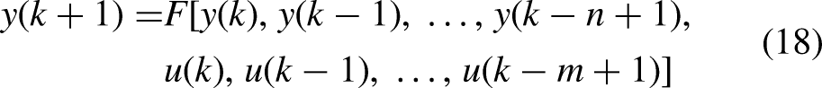
We will develop a neural model using the NFMS architecture for two examples: a second-order nonlinear system and a chemical reactor to display their performances in comparison to single network neural models.

The neural modeling is done using MLPs with one hidden layer and one output.

For partial design, the learning is based on the manual placement of parameters “the centers and the opening of Gaussian functions.” For global design, learning is performed with an online adjustment of all NFMS parameters.

Second-order nonlinear system

First case: Partial design

The mathematical model of the nonlinear system is expressed by the following equation²⁸:

y (k) = u (k - 2) + u (k - 1) + \frac{y (k - 1)}{1 + y^{2} (k - 2)}

(19)

where u(k) and y(k) represent the input signal applied to the process and the output of the system at instant k, respectively.

x(k) = [u(k), u(k − 1), y(k), y(k−1)]: the input vector.

u(k) is assumed to be contained in [0,2]. The training set was composed of 300 examples distributed among the three operating zones (100 examples each).

Zone 1: u(k) varies around the value 0.2 (10%).

Zone 2: u(k) varies around 1 (10%).

Zone 3: u(k) varies around the value 1.8 (10%).

To reduce the number of fuzzy rules, only two inputs have been considered for the fuzzy rules (u(k) and y(k)); they take the form (4).

$A_{i}^{1}$ are fuzzy subsets corresponding to input u. These are represented by Gaussian membership functions centered in $c_{1 i}$ .

$A_{i}^{2}$ are fuzzy subsets corresponding to the output y, and represent Gaussian membership functions centered in $c_{2 i}$ .

The training of the NFMS consists of the training of local models.

The fusion of local models’ outputs gives the output of the NFMS (see equation (5)).

The validity degree $μ_{i}$ is:

μ_{i} = μ_{1 i} . μ_{2 i}

(20)

The initial conditions are selected as follows:

c_{11} = 0.2

c_{12} = 1

c_{13} = 1.8

c_{21} = 0.4

c_{22} = 1.4

c_{23} = 2.4

σ_{1} = 1

, and

σ_{2} = 0.5

. These parameter values were chosen based on previous results and several tests. This is called a supervised initialization.

Several tests have been conducted to determine the learning rate ε and the number of neurons in the hidden layer. The best results were found for ε=0.4 and the number of neurons in the hidden layer was equal to 1 for each NN. The choice of these simulation parameters must guarantee the quality of the learning and convergence times.

For training the NFMS, we trained, simultaneously, and using an iterative process, the weights of the connections of the three networks under the learning algorithm previously described. $c_{j i}$ and $σ_{j}$ are constants during the learning process. After the learning step, to assess the model performance, the evolution of the model and the desired outputs are presented in Figure 6.

Figure 6.

(A) Evolution of the system and the model outputs (partial design). (B) The membership degrees.

This figure shows that the behavior of the model is very similar to that of the system; the system output (represented by the fusion of the local model outputs) and the model output are very similar. For each domain, the membership function of the dominant local network is the highest one. Therefore, the obtained model has a good learning ability.

Model validation was performed by assessing the model performance using the test data and calculating the test error (see Table 1).

Table 1.

Learning results of studied models.

Model	Learning error	Test error	Learning time (s)
Single-network “MLP”	0.0203	0.03	43
“NFMS” with partial design	0.0107	0.0329	20
“NFMS” with global design	0.0029	0.0125	40

MLP: multilayer perceptron; NFMS: neuro-fuzzy modular system.

Second case: Global design

In this case, the training consists of adjusting the weights, centers, and openings of the Gaussian functions.

We used the same learning procedure except the initial values of parameters were random.

The curves of the obtained neural model and system are shown in Figure 7.

Figure 7.

(A) Evolution of the system and the model outputs (global design). (B) Membership degrees.

The system output curve and the model output curve are superposed. Thus, the developed model based on the complete design also gives a good learning ability.

To illustrate the training process, Figure 8 shows the evolution of the center $c_{11}$ at each iteration.

Figure 8.

Evolution of the center c₁₁.

Result analysis

The following table shows the test errors, learning times, and number of hidden neurons. We choose a number of iterations equal to 1000 iterations.

The calculation tool is a personal computer having the characteristics Central Processing Unit@1.7 GHz.

According to Table 1, the NFMS architecture with partial design provides a learning error and a number of hidden neurons lower than NFMS architecture with global design. Regarding the learning time, the NFMS architecture with global design presents a longer time than the others because of the complexity of the algorithm used to adjust the parameters. Therefore, we can conclude that the NFMS architecture with a global design is more rewarding when modeling nonlinear dynamic systems. Finally, we confirm that the random initialization of parameters can ensure a very small error compared with supervised initialization (partial design).

Chemical reactor

Chemical reactors are used to carry out chemical reactions not only in chemical and biochemical engineering but also in the petrochemical industry. The chemical reactions are self-organizing which makes it difficult to predict the behavior of the reactor. Therefore, owing to their strong nonlinear behavior, the identification and control of chemicals remains a challenging task for control engineers. Thus, proper modeling is essential for the design of commercial reactors and the control of their nonlinear chemical processes.⁷¹

We consider a chemical reactor with a Van de Vusse reaction⁷² between two products, A and B. The stirrer works as soon as the reactants enter the tank. Apart from that, the heat exchanger must provide the necessary heat that the reaction requires. This process ends when the reactants become homogeneous. This concept is described in Figure 9.

Figure 9.

Chemical reactor.

The key parameters in a chemical reaction to be considered are temperature, pH, and concentration.

The dynamic behavior of a chemical reactor is represented by the following mathematical nonlinear input equation⁷³:

\begin{aligned} y (k + 1) = & d_{1} + d_{2} u (k) + d_{3} y (k) + d_{4} u {(k)}^{3} \\ + d_{5} y (k - 1) u (k - 1) u (k) \end{aligned}

(20)

Input u(k) represents the incoming flow of product A at time t = kT. Values were normalized between 0 and 1.

Output y(k) represents the concentration of product B at t = kT.

The concentration of product B is always in the interval [0.65,1.05] because the reaction between Van de Vusse and its inverse must be stable.

D = [d₁, d₂, d₃, d₄, d₅]^T= [0.558, 0.583, 0.0116, −0.127, −0.034]^T.

The developed model will enable us to set up different changes in various parameters and predict the system behavior under different complex industrial operating conditions.⁷⁴

First case: Partial design

The modeling of the chemical reactor is performed by training an “NFMS,” which follows these conditions:

x(k) = [u(k), u(k − 1), y(k), y(k − 1)] is the input vector. u(k) denotes a set of random values. The values of the 200 examples vary in [0, 1]. This input is divided into two operating areas, each representing a subsystem, and is set to 100 points.

Zone 1: u(k) varies around the value 0.2 (i.e. 10%).

Zone 2: u(k) varies around the value 0.7 (i.e. 10%).

The output of the system that must be taken in the interval [0.65, 1.05] is defined by equation (20).

Only u(k) and y(k) were used for the fuzzy rules. They take the form of equation (4):

A¹_i are fuzzy subsets associated with the input signal and are characterized by Gaussian membership functions centered in $c_{1 i}$ .

A² _i are fuzzy subsets associated with the output signal and are characterized by Gaussian membership functions centered in $c_{2 i}$

The validity degree $μ_{i}$ takes the form of equation (6).

The initial conditions chosen are $c_{11} = 0.2$ , $c_{12} = 0.7$ , $c_{21} = 0.7$ , $c_{22} = 1$ , $σ_{1} = 0.8$ , and $σ_{2} = 0.1$ .

The output of the “NFMS” takes the form of (5).

One hidden neuron is chosen.

The learning rate ε is 0.4.

The learning algorithm, whose principle is described above, was used to identify the NFMS.

The training results are shown in Figure 10.

Figure 10.

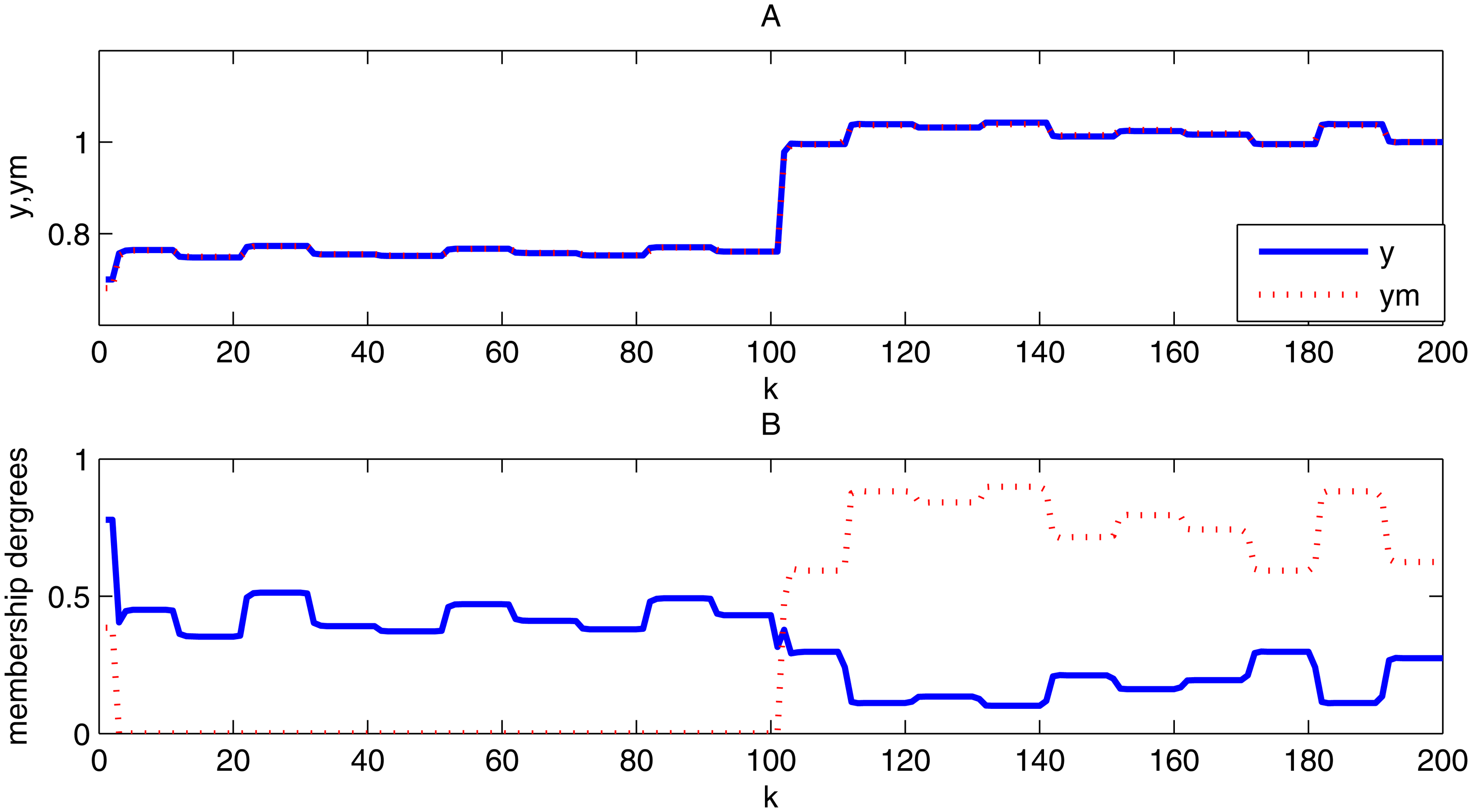
(A) Evolution of the system and the model outputs (partial design). (B) The membership degrees.

The similarity of both the system and model behavior indicates that the chemical reactor has good learning ability.

Second case: Global design

In this case, we adjusted the centers and openings of the Gaussians with weights during learning.

The learning procedure takes the same form as in the first case; however, we suppose that the initial parameters are random. After learning, we obtained the following results.

Figure 11 shows the evolution of the model outputs with the system outputs after the learning step.

Figure 11.

(A) Evolution of the system and the model outputs (global design). (B) The membership degrees.

To illustrate the learning process results, we visualize the variations in the center $c_{21}$ at each iteration in Figure 12.

Figure 12.

Evolution of the center c₂₁.

Model validation was accomplished by evaluating the performance of the model using test data and calculating the test error (Table 2).

Table 2.

Learning results of studied models.

Model	Learning error	Test error	Learning time (s)
Single-network “MLP”	0.0106	0.01	41
“NFMS” with partial design	0.0035	0.0014	24
“NFMS” with global design	0.0030	0.012	28

MLP: multilayer perceptron; NFMS: neuro-fuzzy modular system.

Result analysis

The following table shows the test error, learning time, and number of hidden neurons for 1000 iterations. The same calculation as that in the last example tool was used.

According to Table 2, the learning error and number of hidden neurons in the global design are lower than those in the partial design. However, the learning time of the global design is longer owing to the complexity of the parameter training algorithm. The test error values for the different designs were acceptable. So, having an NFMS architecture with global design is a real gain. The random initialization of parameters can also be more efficient in obtaining good results compared with supervised initialization.

Conclusion

For many engineering requirements, especially the control requirements of complex systems, this paper proposes an NFMS architecture for modeling nonlinear systems based on a neuro-fuzzy approach and a modular structure. We use a TS fuzzy system, where the conclusion is not a linear system, but a nonlinear one, which is a feedforward NN. This approach has been tested using two examples: a numerical example and a real system that is widely used in industry. Despite the ability of NNs to model complex nonlinear structures, there are some problems that make this difficult, such as the number of iterations, number of hidden neurons, and learning rate. Simulation results have shown that when decomposing a complex task into smaller and simpler tasks the learning becomes faster and the error of convergence is lower compared to the learning of the whole system. Moreover, the combination of the local networks using FS techniques heightened the performance. Hence, we can guarantee the effectiveness of the NFMS architecture; the concept of modularity reduces the complexity of the problem, and the neuro-fuzzy combination achieves much better performance. Finally, this technique can be more efficient when we adjust the parameters of the NFMS architecture and the number of local models used during the learning procedure. To implement this idea, we can use incremental learning for the number of local models and hidden numbers. So, the NFMS architecture can really solve many complex nonlinear problems and provide good results, especially in the case of modeling.

Footnotes

Declaration of conflicting interests

The authors declared no potential conflicts of interest with respect to the research, authorship, and/or publication of this article.

Funding

The authors received no financial support for the research, authorship, and/or publication of this article.

ORCID iD

Amina Turki

References

Javeed

Baleanu

Nawaz

, et al. Soliton solutions of nonlinear Boussinesq models using the exponential function technique. Phys Scr 2021; 96: Article 105209.

Sabir

Raja

MAZ

Javeed

, et al. Numerical investigations of a fractional nonlinear dengue model using artificial neural networks. Fractals 2022; 30: 2240241.

Umar

Sabir

Raja

MAZ

, et al. A novel study of Morlet neural networks to solve the nonlinear HIV infection system of latently infected cells. Results Phys 2021; 25: 104235.

Sabir

Umar

Asif

, et al. Numerical solutions of a novel designed prevention class in the HIV nonlinear model. Comput Model Eng Sci 2021; 129: 227–251.

Ksantini

Ellouze

Delmotte

. Control of a hydraulic system by means of a fuzzy approach. Int J Optim Control: Theor Appl 2013; 3: 121–131.

Ksantini

Taieb

Hammami

, et al. Asymptotic behavior of Takagi-Sugeno fuzzy control systems with bounded uncertainties. In: 2019 16th international multi-conference on systems, signals & devices (SSD), IEEE, Istanbul, Turkey, 21–24 March 2019, pp. 108–112.

Stylios

Groumpos

. Modeling complex systems using fuzzy cognitive maps. IEEE Trans Syst Man Cybern A Syst Hum 2004; 34: 155–162.

Takagi

Sugeno

. Fuzzy identification of systems and its applications to modeling and control. IEEE Trans Syst Man Cybern 1985; 15: 116–132.

Deng

Choi

Cao

, et al. T2FELA: Type-2 fuzzy extreme learning algorithm for fast training of interval type-2 TSK fuzzy logic system. IEEE Trans Neural Netw Learn Syst 2014; 25: 664–676.

10.

Jiang

Chung

F-L

Ishibuchi

, et al. Multitask TSK fuzzy system modeling by mining intertask common hidden structure. IEEE Trans Cybern 2015; 45: 534–547.

11.

Guerra

Ksontini

Delmotte

. Some new relaxed conditions of quadratic stabilization for continuous Takagi-Sugeno fuzzy models. In: Proceedings of the IEEE CESA 2003, IEEE CESA '03, 12 July, Lille, France, vol. 3.

12.

Feng

. A survey on analysis and design of model-based fuzzy control systems. IEEE Trans Fuzzy Syst 2006; 14: 676–697.

13.

, et al. Concise fuzzy system modeling integrating soft subspace clustering and sparse learning. IEEE Trans Fuzzy Syst 2019; 27: 2176–2189.

14.

Javed

Javeed

Ahmad

, et al. Approach to multi-attribute decision-making problems based on neutrality aggregation operators of picture fuzzy information. J Funct Spaces 2022; 2022: 2762067.

15.

Javed

Javeed

Ullah

, et al. Approach to multi-attribute decision-making problems based on neutrality aggregation operators of T-spherical fuzzy information. Comput Appl Math 2022; 41: 10.

16.

Elfelly

Dieulot

Benrejeb

, et al. A new approach for multimodel identification of complex systems based on both neural and fuzzy clustering algorithms. Eng Appl Artif Intell 2010; 23: 1064–1071.

17.

Orjuela

Marx

Ragot

, et al. A decoupled multiple model approach for state estimation of nonlinear systems subject to delayed measurements. In: Third IFAC workshop on advanced fuzzy and neural control, Valenciennes, France. 29–30 October 2007 pp. 97–102. Elsevier, Springer.

18.

Singh

Tyagi

Kumar

. Application of neural network based control strategies to binary distillation column. J Control Eng Appl Inf 2013; 15: 47–57.

19.

Sabir

Umar

Guirao

JLG

, et al. Integrated intelligent computing paradigm for nonlinear multi-singular third-order Emden–Fowler equation. Neural Comput Appl 2021; 33: 3417–3436.

20.

Sabir

Wahab

Umar

, et al. Stochastic numerical approach for solving second order nonlinear singular functional differential equation. Appl Math Comput 2019; 363: 124605.

21.

Suantai

Sabir

Umar

, et al. Scaled conjugate gradient for the numerical simulations of the mathematical model-based monkeypox transmission. Fractal Fract. 2023; 7: 63.

22.

Souayeh

Sabir

Umar

, et al. Supervised neural network procedures for the novel fractional food supply model. Fractal Fract 2022; 6: 33.

23.

Umar

Amin

Salahshour

, et al. Swarming computational approach for the heartbeat van der Pol nonlinear system. Computers. Mater Contin. 2022; 72: 6186–6202.

24.

Andonie

Kovalerchuk

. Neural networks for data mining: Constrains and open problems. In: European symposium on artificial neural networks, Bruges, Belgium, 28–30 April 2004, pp. 449–458. d-side publi.

25.

Baruch

Beltran-Lopez

Guzman

JLO

, et al. A fuzzy-neural multi-model for nonlinear systems identification and control. Fuzzy Sets Syst 2008; 159: 2650–2667.

26.

Narendra

Parthasarathy

. Identification and control of dynamical systems using neural networks. IEEE Trans Neural Netw 1990; 1: 4–27.

27.

Alaloul

Qureshi

. Data processing using artificial neural networks. In: Harkut

(ed.) Dynamic data assimilation – beating the uncertainties. London, United Kingdom: IntechOpen, 2020, pp. 118.

28.

Abiodun

Jantan

Omolara

, et al.

State-of-the-art in artificial neural network applications: a survey.

Heliyon 2018; 4: e00938.

29.

Beatriz

Fevrier

Patricia

, et al.

Fuzzy logic in the gravitational search algorithm enhanced using fuzzy logic with dynamic alpha parameter value adaptation for the optimization of modular neural networks in echocardiogram recognition.

Appl Soft Comput 2015; 37: 245–254.

30.

Chen

. Chapter 28, Deep and modular neural networks. In: Chen

(ed.) Springer handbook of computational intelligence. Berlin, Heidelberg: Springer, 2015, pp. 473–494.

31.

Viharos

Kis

. Survey on neuro-fuzzy systems and their applications in technical diagnostics and measurement. Measurement 2015; 67: 126–136.

32.

Carbureanu

. The development of a neuro-fuzzy expert system for wastewater pH control. Control Eng Appl Inf 2014; 16: 30–41.

33.

Kumar

Gaur

Mittal

. Novel ai based on-line sequential learning technique for high performance DC servo motor control. Control Eng Appl Inf 2015; 17: 3–11.

34.

Tiruneha

Fayekb

Sumati

. Neuro-fuzzy systems in construction engineering and management research. Autom Construct 2020; 119: 103348.

35.

Patricia

. Chapter 7. Signature recognition with a hybrid approach combining modular neural networks and fuzzy logic for response integration. In: Raja

(ed.) Modular neural networks and type-2 fuzzy systems for pattern recognition. Berlin, Heidelberg: Springer, 2012, pp. 77–92.

36.

Ronco

Gawthrop

. Modular neural networks: a state of the art. Technical report. Centre for System and Control, University of Glasgow, UK, 1995.

37.

Ronco

Gawthrop

. Gated modular neural networks for control oriented modelling. Technical report. Centre for System and Control, University of Glasgow, UK, 1998.

38.

Auda

Kamel

. Modular neural networks: A survey. Int J Neural Syst 1999; 9: 129–151.

39.

Jenkins

Yuhas

. A simplified neural network solution through problem decomposition: The case of the truck backer-upper. IEEE Trans Neural Netw 1993; 4: 718–722.

40.

Thiria

Mejia

Badran

, et al. Multimodular neural architecture for remote sensing operations. Adv Neural Inf Process Syst 1991; 4: 675–682.

41.

B-L

Ito

. Task decomposition and module combination based on class relations: a modular neural network for pattern classification. IEEE Trans Neural Netw Sept. 1999; 10: 1244–1256.

42.

Robert

Michael

Steven

, et al. Adaptive mixtures of local experts. Neural Comput 1991; 3: 79–87.

43.

Chiang

. A divide-and-conquer methodology for modular supervised neural network design. In: World congress on computational intelligence. Orlando, Florida, USA, 28 June–6 July 1994, pp. 119–124, IEEE.

44.

Zein-Sabatto

Hwang

Marpaka

. Neural networks sharing knowledge and experience. In: World congress on computational intelligence 1994, Orlando, Florida, USA, 28 June–6 July 1994, pp. 613–618, IEEE.

45.

Venkateswaran

Obradovic

. Efficient learning through cooperation. In: Raja

(ed.) World congress on computational intelligence, pp. 390–395.

46.

MacLeod

Maxwell

Muthuraman

. Incremental growth in modular neural networks. Eng Appl Artif Intell 2009; 22: 660–666.

47.

Deshmukh

Ghatol

. Modular neural network approach for short term flood forecasting a comparative study. Int J Adv Comput Sci Appl 2010; 5: 81–87.

48.

. Rainfall time series forecasting based on modular RBF neural network model coupled with SSA and PLS. J Theor Appl Comput Sci 2012; 6: 3–12.

49.

Auda

Kamel

Raafat

. Modular neural network architectures for classification. In: Proceedings of International Conference on Neural Networks (ICNN'96). Washington, DC, USA, 1996.

50.

Talmoudi

Abderrahim

Abdennour

, et al. Multimodel approach using neural networks for complex systems modeling and identification. Nonlinear Dyn Syst Theory 2008; 8: 299–316.

51.

Kamel

Xia

. Cooperative recurrent modular neural networks for constrained optimization: A survey of models and applications. Cogn Neurodyn 2009; 3: 47–81.

52.

Snchez

Melin

Castillo

. A new model of modular neural networks with fuzzy granularity for pattern recognition and its optimization with hierarchical genetic algorithms. In: Advances in soft computing. Lecture notes in computer science. Batyrshin and G. Sidorov (Eds.): MICAI 2011, Part II, LNAI 7095, pp. 331–342, Berlin, Heidelberg: Springer, 2011.

53.

Khare

Yao

Sendhoff

, et al. Co-evolutionary modular neural networks for automatic problem decomposition. IEEE Congr Evolut Comput 2005; 3: 2691–2698.

54.

Vieira

Dias

Mota

. Neuro-fuzzy systems: a survey. In: 5th WSEAS NNA International conference on neural networks and applications. Udine, Italia, 25–27 March 2004, pp. 414–419.

55.

Malek

Ebadzadeh

Rahmati

. Three new fuzzy neural networks learning algorithms based on clustering, training error and genetic algorithm. Appl Intell 2012; 37: 280–289.

56.

Nauck

Kruse

. Neuro-fuzzy systems for function approximation. Fuzzy Sets Syst 1999; 101: 261–271.

57.

Abraham

. Neuro fuzzy systems: state-of-the-art modeling techniques. In: Connectionist models of neurons, learning processes, and artificial intelligence. IWANN 2001. Lecture Notes in Computer Science. Berlin, Heidelberg: Springer, J. Mira and A. Prieto (Eds.): IWANN 2001, LNCS 2084, 2001, pp. 269–276.

58.

Pedrycz

Card

. Linguistic interpretation of self-organizing maps. In: IEEE international conference on fuzzy systems, San Diego, CA, USA, 08–12 March 1992, pp. 371–378. IEEE.

59.

Guney

Sarikaya

. Concucurrent neuro-fuzzy systems for resonant frequency computation of rectangular, circular, and triangular microstrip antennas. Prog Electromagn Res 2008; 84: 253–277.

60.

Lin

Lee

CSG

. Neural-network-based fuzzy logic control and decision system. IEEE Trans Comput 1991; 40: 1320–1336.

61.

Ioana

. Modeling, identification and prediction of inherent quasi-stationary pressure dynamics of a common-rail system using neuro-fuzzy structures with local linear arx models. J Control Eng Appl Inf 2012; 14: 61–70.

62.

Jang

. Neuro-fuzzy modeling: architectures, analyses and applications. PhD Thesis, University of California,

Berkeley

, 1992.

63.

Berenji

Khedkar

. Learning and tuning fuzzy logic controllers through reinforcements. IEEE Trans Neural Netw 1992; 3: 724–740.

64.

Tano

Oyama

Arnould

. Deep combination of fuzzy inference and neural network in fuzzy inference. Fuzzy Sets Syst 1996; 82: 151–160.

65.

Sulzberger

Tschichold-Gurman

Vestli

. FUN: Optimization of fuzzy rule based systems using neural networks. In: IEEE international conference on neural networks, San Francisco, CA, USA, 28 March–01 April 1993; vol. 1, pp. 312–316. IEEE.

66.

Juang

Lin

. An online self-constructing neural fuzzy inference network and its applications. IEEE Trans Fuzzy Syst 1998; 6: 12–32.

67.

Kasabov

Qun

. Dynamic evolving fuzzy neural networks with ‘m-out-of-n’ activation nodes for on-line adaptive systems, Technical report. Department of Information Science, University of Otago, 1999.

68.

Turki

Chtourou

Djemel

. Multi-model neural approaches for nonlinear systems modeling. Trans Syst Signals Devices 2013; 8: 21–39.

69.

Turki

Chtourou

. Multi-network neural model for nonlinear systems modeling. In: 23rd international symposium on industrial electronics. Istanbul, Turkey, 01–04 June 2014, pp. 162–166. IEEE.

70.

Hornik

. Approximation capabilities of multilayer feedforward networks. Neural Netw 1991; 4: 251–257.

71.

Burghardt

. Ideal models of reactors. Chem Eng Chem Process Technol 2010; 3: 1–46.

72.

Van de Vusse

. Plug-flow type reactor versus tank reactor. Chem Eng Sci 1964; 19: 994–996.

73.

Hernandez

Arkun

. Stability of nonlinear polynomial ARMA models and their inverse. IBM J Res Dev 2000; 44: 725–747.

74.

Hussaina

Blanka

Elbashir

. Modeling the fixed-bed Fischer–Tropsch reactor in different reaction media computer aided chemical engineering. Comput Aided Chem Eng 2015; 37: 143–148.

A neuro-fuzzy modular system for modeling nonlinear systems

Abstract

Keywords

Introduction

Related works

Modular neural networks

Neuro-fuzzy systems

The neuro-fuzzy modular system

General description and architecture

Training algorithm

Partial design

Global design

Nonlinear dynamic system using the “NFMS”

Second-order nonlinear system

First case: Partial design

Second case: Global design

Result analysis

Chemical reactor

First case: Partial design

Second case: Global design

Result analysis

Conclusion

Footnotes

Declaration of conflicting interests

Funding

ORCID iD

References