Addressing the class imbalance in tabular datasets from a generative adversarial network approach in supervised machine learning

Abstract

One common issue with datasets used for supervised classification tasks is data imbalance or the unequal distribution of classes within a dataset. The class imbalance may cause biased machine learning models to favor the dominant class, misclassifying the minority class. Specific techniques can be employed to deal with the issue of class imbalance, including resampling by oversampling or undersampling and ensemble approaches. Besides, generative adversarial networks, a deep learning technique for building generative models, offer an alternative machine learning technique that is particularly well suited to address the class imbalance problem. This work introduces a machine learning-based approach to deal with the class imbalance in a cancer intracellular signaling dataset produced by a verified and validated computer simulation. Specifically, we use synthetic data generation to increase and balance the dataset generated by the computational simulation. The used approach simulates the oversampling method by employing a generative adversarial network to produce new examples for the minority class. Subsequently, we applied supervised machine learning methods, such as the K-NN algorithm, to assess whether or not the classification accuracy improved relative to the unbalanced dataset. The results presented in this work have shown an accuracy increase in the classification of patterns belonging to the minority class, with an improvement of $24.5\mathrm{\%}$ .

Introduction

When supervised classification tasks are tackled using machine learning, two major issues arise: (a) The vast number of features that must be dealt with and (b) the problem of class imbalance.

Regarding the first problem, when a machine learning-based classification model is built from a dataset, the dataset is expected to provide the model with features relevant to the classification task. However, there is a chance of introducing unnecessary noise and reducing the accuracy of the model if the features entered into the model are irrelevant. When data have many dimensions, two potential problems could occur: (a) the model may be overfitted and perform poorly if there are more characteristics than observations, and (b) when there are many features, it is harder to group the data; too many dimensions make every observation in the corpus appear to be equally spaced from every other observation. Additionally, since Euclidean distance is frequently utilized by grouping techniques to assess the similarity between observations, this poses a challenge because no meaningful clusters can be formed if all distances are roughly equal. In data mining, feature selection or dimensionality reduction is the technique for tackling this problem. Standard filter methods, e.g., Pearson’s Correlation and Chi,^1,2 wrapper methods, e.g., Recursive Feature Elimination, ³ and embedded methods, e.g., Least Absolute Shrinkage and Selection Operator (LASSO) and Tree-based Feature Selection, ⁴ are commonly employed for feature selection. ⁵

Regarding the second issue, data imbalance, or the unequal distribution of classes within a dataset, is a typical problem with datasets used for supervised classification tasks. Machine learning models may become biased in favor of the dominant class as a result of the class imbalance misclassifying the minority class. Specific techniques can be used to alleviate the issue of class imbalance, including resampling by oversampling or undersampling ⁶ and ensemble approaches. ⁷ Oversampling can be accomplished by selecting the value that occurs most frequently in the class and repeating it, randomly selecting a value from the smallest class, or producing as many synthetic samples as required. On the other hand, undersampling is a technique that decreases the number of samples from the largest classes to the smallest class size. When these two approaches are combined, the majority class can be undersampled and the minority class oversampled. Ensemble approaches, on the other hand, frequently use boosting or bagging to develop several estimators on various randomly chosen subsets of data.

Alternatively, another machine learning technique that is very suitable to treat the problem of class imbalance is that of Generative Adversarial Networks (GANs), ⁸ a deep learning technique to train generative models. GANs often comprise a generator and a discriminator that learn simultaneously. The aim of GANs is to estimate the potential distribution of real data samples and generate new samples from that distribution. A GAN typically consists of two parts: A generator (G) and a discriminator (D), both of which learn simultaneously. In order to create new data from this hypothetical distribution of real samples, G aims to capture the distribution of a particular dataset. On the other hand, D’s responsibility is to reliably distinguish generated samples from real data, often with the help of a binary classifier.

In a previous study, ⁹ we dealt with the dimensionality reduction of a cell signaling dataset for multiclass classification tasks by using a group of feature selection techniques, including Low variance, Chi-Squared, Recursive feature elimination, the LASSO, Tree-based feature selection, and Pearson’s correlation. The results produced by the dimensionality reduction analysis based on this group of feature selection techniques showed the importance or weight of eight predictive attributes (signaling elements) from the whole set of 16 attributes. The subsets of characteristics chosen by the Chi-Square and Tree-based feature selection techniques (each formed by eight features) produced the highest accuracy in the multiclass classification task. With $k=6$ , the k-NN algorithm obtained an accuracy rating of 99.65% for the eight features chosen via the Chi-Square approach. On the other hand, the accuracy rate for the group of eight features picked using the Tree-based Feature Selection technique was 99.75% for $k=2$ .

Despite the excellent accuracy obtained in the supervised classification task when dimensionality reduction was considered, another problem that still needs to be addressed in this cell signaling dataset is class imbalance. The fundamental issue with our imbalanced signaling dataset is that the minority class had insufficient samples for the machine learning algorithm to learn the decision boundary successfully. Specifically, the minority class is almost 30 times smaller than the majority class, which may result in a machine learning model biased (in this case, k-NN algorithm) for the dominant class.

In this work, we present a machine-learning-based approach to address the class imbalance in the cell signaling dataset previously referred to and presented in González-Pérez and Sánchez-Gutiérrez. ⁹ In this approach, we use a conditional tabular GAN (ctGAN) to generate new instances for the minority class as if using the oversampling technique. We aim to assess how much the accuracy of supervised classification can be improved by using dimensionality reduction in conjunction with class balancing. Subsequently, we apply data mining and machine learning methods to the balanced cell signaling dataset to obtain new inferences and knowledge about this important biological system.

The utilization of ctGAN aligns with the broader trend in computational biology toward leveraging advanced machine learning techniques for data augmentation and enhancement. Recently, there has been a growing recognition of the potential benefits of generative models. This is particularly pertinent in overcoming data scarcity issues in domains such as cell signaling, where acquiring extensive experimental data can be resource-intensive and time-consuming. The ctGAN model, with its capacity to generate biologically plausible samples, complements existing approaches by providing a means to expand datasets in a principled and data-driven manner. This not only mitigates class imbalance but also contributes to a more comprehensive and representative characterization of cellular behavior.

Furthermore, the application of ctGAN in this context highlights the interdisciplinary nature of modern bioinformatics research. By integrating techniques from computer science, statistics, and bioinformatics, this study exemplifies the synergistic potential of cross-disciplinary collaboration. The ctGAN model, originally developed in the context of GANs, finds a novel application in addressing a fundamental issue in cellular biology. This convergence of expertise underscores the dynamic and evolving nature of research methodologies and the adaptability of advanced machine learning tools to diverse scientific domains.

Material and methods

Methodological approach to producing synthetic data

Our methodological approach to producing high-fidelity synthetic data for enhancing data generated by the computational simulation involves the following phases:

Start from a calibrated, verified, and validated cell signaling network simulation tool.

Use the data farming method to produce large volumes of data resulting from the execution of the simulation.

Carry out the data preparation for machine learning.

Address the class imbalance problem by generating synthetic data with an approach based on GANs.

Conduct a qualitative and quantitative analysis of the synthetic data produced.

Perform an exploratory data analysis (EDA), emphasizing the feature selection.

Execute the multi-class classification machine learning technique.

Examine the results.

Figure 1 shows the phases of the proposed methodological approach and the flows that should commonly be followed. This work emphasizes phases 3 to 5, 7 and 8.

Figure 1.

The phases of our methodological approach to produce synthetic data. Note that solid arrows mean forward flow between a preceding and succeeding phase, while dashed arrows denote backward flow to a given preceding phase. Note that the Running the simulation, Data farming Method, Data preparation, and EDA phases will not be treated in this work since these were already addressed in a previous study. ⁹

The data farming process and the synthetic data technique

An increasingly relevant application of computer simulation is the concept of “data farming.” This term refers to generating and cultivating large amounts of data using computer simulations. Like traditional agriculture, which involves raising animals or growing plants, data farming aims to gather valuable data through computer-simulated experiments. The basis of data farming is the notion that data produced by computer simulations can be just as rich and priceless as data gathered through physical experiments.

One of the main advantages of data farming is its ability to quickly generate large volumes of data. While physical experiments often require hours, days, weeks, or even months to collect enough data, computer simulations can generate data much faster. Those simulations allow researchers to explore various settings and conditions relatively quickly, speeding up the research and discovery process.

Despite the many advantages of data farming through computer simulation, there are still issues with the reliability and consistency of the data produced. There is a chance of adding bias or inaccuracies to computer simulations as models and algorithms become more complicated. These mistakes may result from faulty software, skewed assumptions, or using the wrong parameters. Therefore, validating and verifying models, software, and input data is essential to ensure their quality.

In this work, we use the computer simulation of intracellular signaling networks to:

Observe, explore, and understand the behavior of a particular cell signaling network when the simulation has been calibrated, verified, and validated.

Perform a wide range of in silico experiments to guide subsequent in vitro experimentation.

Produce large volumes of data (data farming) that describe the evolution and behavior of the cell signaling network over time for subsequent analytic processes based on machine learning techniques.

Note that data produced by the computational simulation is structured in rows and columns, where the first $m-1$ columns of each record correspond to the predictive characteristics, and the $m$ th column denotes the class or category. Each predictive characteristic represents the active/non-active concentration level of a particular element belonging to the signaling network. At the same time, the class or category denotes a particular combination of cellular processes associated with this activation pattern.

On the other hand, synthetic data is artificially generated data that closely resembles ground truth data but does not come from direct observations, nor is it the result of running computer simulations. This data is produced using generation techniques such as synthetic minority over-sampling technique (SMOTE), GANs, or interpolation algorithms. Synthetic data is most useful when genuine data is scarce, private, or difficult to obtain. Furthermore, synthetic data is valuable when a class imbalance problem or an imbalanced dataset is at hand in the data generated by the computational simulation. The ability of synthetic data to supplement small or imbalanced datasets and improve the classification of machine learning models has made it popular across many fields.

The cell signaling dataset

In a previous study, ⁹ we tackled the dimensionality reduction in a supervised multiclass classification task using a cancer cell signaling dataset harvested (through the data farming process) from a computer simulation carried out by the Big Data Cellulat bioinformatics simulation tool.^10–14 In this study, we revisit this cell signaling dataset to tackle the issue of class imbalance in supervised multiclass classification. The instances in this dataset describe the activation state of cell signaling components (e.g., receptors, proteins, and enzymes) into classes that symbolize the different cellular processes (e.g., survival, proliferation, motility) triggered in cancer cells.

Table 1 displays the properties of the cell-signaling dataset regarding the number of classes, instances, and features. The dataset consists of $2195$ cases, each identified by 16 input attributes, five output attributes, and a final attribute representing the class or category. The 16 predictive features indicate the concentration value of the signaling components, such as tumor suppressor proteins, key proteins, anti-apoptotic proteins, pro-apoptotic proteins, and receptors. The level of activity of the cellular processes corresponding to a particular activation state of the signaling elements is represented by the five output attributes. The last attribute, representing the class, takes values from 1 to 6. As can be seen in Table 2, each of these classes represents a particular combination of the following cellular processes: survival, proliferation, motility, epithelial-mesenchymal transition (EMT), and apoptosis.

Table 1.

Cell signaling dataset produced by the Big-Data Cellular bioinformatics simulator.

Dataset	Number of predictive instances	Number of output features	Number of attributes representing the class	Number of instances
Cancer cell signaling pathway	16	5	1	2195

Table 2.

Classification scheme.

Cellular processes					Class
Survival	Proliferation	Motility	Epithelial-mesenchymal transition (EMT)	Apoptosis
1	0	0	0	0	1
1	1	0	0	0	2
1	1	0	1	0	3
1	1	1	1	0	4
1	1	1	0	0	5
0	0	0	0	1	6

As a result of the activation/inactivation states of the signaling components that comprise the cell signaling pathway, the classes shown in the last column represent various combinations of cellular states that the cell can attain. Class 1 is survival; Class 2 is proliferation and survival; Class 3 is survival, proliferation and EMT; Class 4 is survival, proliferation, motility and EMT; Class 5 is survival, proliferation and motility; and Class 6 is apoptosis.

Figure 2 shows the number of instances assigned to each of the six classes identified in Table 2. This figure demonstrates a significant class imbalance in the dataset, with the minority class (class 3) being nearly 30 times smaller than the dominant class (class 1). As was already established, a class imbalance might result in biased machine learning models favoring the dominant class, misclassifying the minority class.

Figure 2.

The problem of class imbalance. In the cancer signaling dataset, the minority class is roughly 30 times smaller than the majority class, leading to an imbalance class problem.

Generative adversarial networks

GANs ⁸ are a deep learning technique for building generative models and have become widely utilized in recent years to generate realistic images. Here, we use the generative capacity of these networks to augment the number of occurrences in a dataset, specifically to address the class imbalance problem. GANs are used to create new samples by estimating the distribution that real data samples might have in the future.

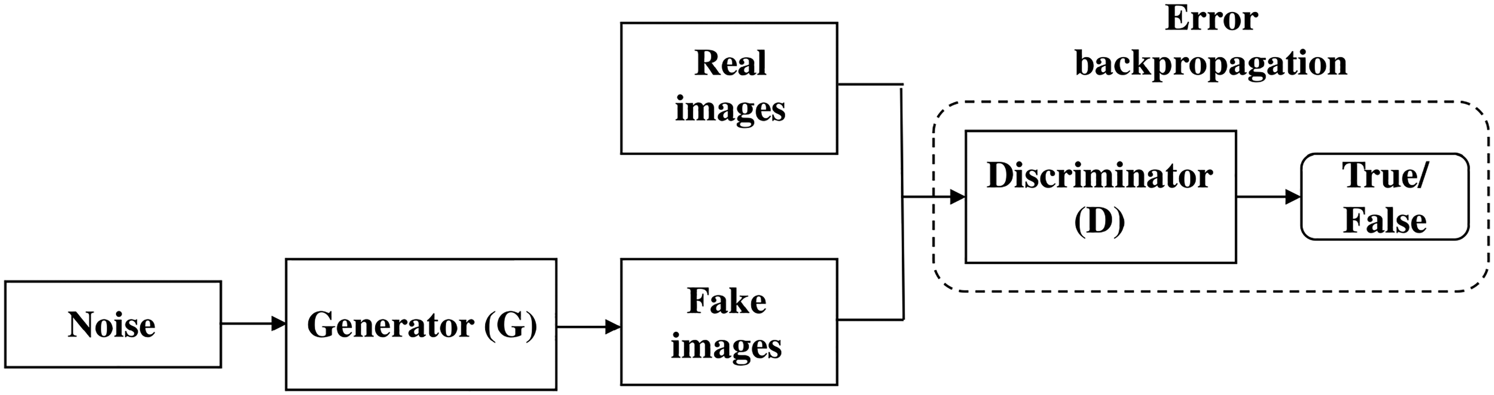
As shown in Figure 3, commonly, a GAN involves two components, a generator (G) and a discriminator (D), both learning simultaneously. On the one hand, the goal of G is to capture the distribution of a particular dataset and produce new data from this potential distribution of real samples. On the other hand, the job of D is to accurately discriminate real data from generated samples, typically through a binary classifier. In other words, by comparing the data that G generates to real data, D contributes to the training of G by teaching it about the distribution that underlies the real data.

Figure 3.

Both the generator and the discriminator components are neural networks. The generator output is connected directly to the discriminator input. Through backpropagation, the discriminator’s classification provides a signal that the generator uses to update its weights.

The discriminator component

In a GAN, the discriminator component (D) is a neural network trained to take in samples and predict whether they are real or fake. For example, if the GAN is being trained to generate images, the discriminator might be fed both real and fake images generated by the generator. Based on its training, it would try to predict which images are real or fake. The goal of the discriminator is to become as accurate as possible at distinguishing real from fake samples. As the generator improves at producing realistic samples, the discriminator must become more sophisticated to keep up. This competition drives both parts of the GAN to improve, ultimately resulting in the generator being able to produce highly realistic samples.

The discriminator is trained on a real-world sample dataset. For example, if the GAN is being trained to generate images, the discriminator would be trained on a dataset of real images. The generator component’s fake samples are the discriminator’s second source of training data (G). As G improves at producing realistic samples, D is fed more of these bogus samples, which it uses to improve its ability to distinguish between real and bogus. That is, the discriminator’s training data comes from both real-world and fake samples generated by the generator.

The boxes labeled “Real images” and “Fake images” in Figure 4 depict the data sources used to train the discriminator. The real-world samples are one source, and the generator’s fake samples are another. The generator’s weights do not change during the discriminator training. Instead, it creates fake samples for the discriminator to use for training while keeping its weights constant.

Figure 4.

Backpropagation in discriminator training.

The discriminator is connected to two loss functions (not shown in Figure 4). During its training, it uses only the loss function associated with the discriminator itself, ignoring the generator loss function. This is because the generator’s loss function is used only during the training of the generator, which is a separate process addressed in the next section.

The generator component

The generator part of a GAN is a neural network that takes in random noise as input and generates samples that are meant to be indistinguishable from real-world data. For example, if the GAN is being trained to generate images, the generator might take in random noise and produce images that look realistic to a human observer. The generator’s training involves competing with the discriminator, intending to produce samples that fool the discriminator into thinking they are real.

As shown in Figure 5, the generator usually consists of several layers of neurons; these combine to transform the random noise input into an output similar to the real-world data and improve the quality of its generated samples.

Figure 5.

Backpropagation and optimization algorithms in generator training.

Training the generator in a GAN requires a closer connection between the generator and the discriminator than is necessary for training the discriminator alone.

In its most basic configuration, the generator receives an input of random noise and creates fake samples using that input. As the first step in the generating process, the random noise gives the generator the variation and randomness it needs to create a wide variety of fake samples. Depending on the kind of data the GAN is being trained to produce, the precise form of the random noise input can change. For instance, the random noise input may be a tensor of random numbers with the same dimensions as the training images if the GAN is being trained to create images. The generator needs this input to produce various fake samples and enhance its performance.

When a neural network is trained, its weights are often changed to lessen the error or loss in the output. The loss we seek to reduce in a GAN is not directly tied to the generator. Instead, the output from the generator is sent into the network of the discriminator, which then creates the output signal. The generator is penalized by its loss function for creating samples that the discriminator labels as fake. As a result, the generator is motivated to create more realistic samples that deceive the discriminator.

The GAN approach for tabular data

Several potential motivations exist for using a GAN to generate tabular data, such as datasets with rows and columns of numerical values. A potential use case includes generating synthetic samples for training and evaluating machine learning models. In this respect, a GAN can be trained on a real-world dataset and then used to generate new, synthetic examples similar to the original data. This can be useful for training machine learning models, especially when the original dataset is small or insufficient for the desired task. A GAN can be used to generate additional samples that are similar to the real data but with added randomness or noise. These samples can then augment the original dataset, improving the performance of machine learning models trained on that dataset. In this work, the general idea is to use the GAN’s ability to generate realistic samples based on a real dataset to improve the data’s quality or utility in some way, such as data augmentation. Specifically, our goal is to explore and evaluate the GAN approach to address the problem of class imbalance in classification supervised learning.

The conditional tabular GAN model

A conditional GAN, or cGAN, ¹⁵ is a variant of the GAN architecture that introduces additional input to both the generator and the discriminator. This additional input, called the conditioning information, allows the cGAN to generate samples conditioned on specific characteristics or class labels. For example, a cGAN trained on images of faces could be given a specific gender as conditioning information and then generate fake images of faces that are either male or female, depending on the conditioning input.

A ctGAN, ¹⁶ or ctGAN, is a type of cGAN designed explicitly for generating tabular data, such as datasets with rows and columns of numerical values. Like other cGANs, a ctGAN uses additional conditioning information to produce more specific, controlled samples. In the case of a ctGAN, the conditioning information can be used to specify characteristics of the generated data, such as the type or range of values in each column. In particular, a ctGAN could be used for data augmentation in a cellular signaling dataset like the one we address in this work.

In our example, a ctGAN is trained on a set of instances that represent the various activation/inhibition states of the signaling components that make up the network and uses the conditioning data associated with the cellular process (or class) that corresponds to each instance as a representation of the activation/inhibition state. The ctGAN uses this knowledge to produce further samples comparable to the actual data. The original dataset is supplemented with these created samples, which gives the machine-learning algorithms that interpret the cell signaling data more training data.

The training process for a conditional tabular GAN, or ctGAN, is similar to the training process for a regular GAN, but with the addition of conditioning information. The main steps in the training process for a ctGAN are as follows:

Sample random noise as input for the generator.

Use the generator network to produce fake samples based on the random noise input and the conditioning information.

Feed the fake samples to the discriminator, which makes predictions about whether they are real or fake based on the conditioning information.

Employ the discriminator output (i.e., whether the samples are predicted to be real or fake) to calculate a loss value for the generator. Given the conditioning information, this loss value reflects how well the generator could fool the discriminator with its generated samples.

Apply backpropagation to calculate gradients for the discriminator and the generator based on the generator loss.

Use the gradients to update only the generator’s weights.

Repeat this process for multiple epochs to train the generator to produce highly realistic samples that can fool the discriminator, given the conditioning information.

In Figure 6, the generator is fed with random noise (z) and conditioning information (y) as input from the tabular data (T). The conditioning information can specify characteristics of the generated data, such as the type or range of values in each column. The generator then produces synthetic samples passed to the discriminator (D) for classification. The discriminator predicts whether the sample is real or fake and provides a signal to the generator through backpropagation. The generator uses this signal to update its weights and improve its ability to produce realistic samples. Figure 6 also shows that the discriminator is trained using real data from the original dataset and fake data from the generator. The discriminator uses the classification of these samples to update its weights and improve its ability to distinguish real from fake samples.

Figure 6.

A ctGAN model. The conditional generator can generate synthetic rows of tabular data conditioned on one of the discrete columns. The generator uses “training-by-sampling” to learn from the real data and produces similar distribution samples.

In Xu et al. ¹⁶ the authors present three key elements for the ctGAN: The conditional vector, the generator loss, and the training-by-sampling method. The conditional vector is a mathematical representation of the additional conditioning information used to train the generator network of the ctGAN according to:

Let $k^{*}$ be the value from the $i^{*}$ th discrete column $D_{i^{*}}$ .

The conditional vector is conformed when the condition $D_{i^{*}}=k^{*}$ is met.

Let the discrete columns $D_1,\dots ,D_{N_d}$ be represented as one-hot vectors $d_1,\dots ,d_{N_d}$ such that the $i-th$ one-hot vector is $d_i=[d_i^{(k)}]$ , for $k_1=1,\dots ,|D_i|$ .

Let $m_i=[m_i^{(k)}]$ , for $k_1=1,\dots ,|D_i|$ be the $i-th$ mask vector associated with the $i$ th one-hot vector $d_i$ .

Hence, the condition can be expressed in terms of these mask vectors as:

$$m_i^{\left(k\right)}=\{\begin{array}{cc}1& \text{i}fi=i^{*}\text{ and }k=k^{*}\\ 0& \text{otherwise}\end{array}$$

Since each one-hot vector corresponds to a category column (target) in the original dataset, we may infer from the foregoing that the conditional vector is a concatenation of one-hot column vectors. A one-hot vector is a binary vector with a single 1 signifying the class of the current sample and 0s for all other classes. It has a length equal to the number of classes.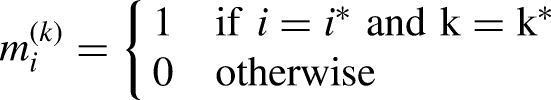

The cross-entropy loss between the true labels and the predicted probabilities generated by the discriminator network is the generator loss. The true labels serve as binary indicators of a sample’s truthfulness, with 1 denoting a genuine sample and 0 denoting a counterfeit sample. The output of the discriminator network is the projected probabilities, which show the likelihood that a given sample is authentic or fraudulent. The discrepancy between the true labels and the predicted probabilities is measured by the binary cross-entropy loss defined as:

$$\begin{array}{c}L=-{\displaystyle \sum _{i=1}^2{y}_{i}log\left(p\right)=-[ylog\left(p\right)+(1-y)log(1-p)]}\end{array}$$

(1)

where $L$ is the cross-entropy loss, $y$ is the true label, $p$ is the predicted probability, and log is the natural logarithm.

Finally, training-by-sampling is based on resampling the original dataset in a way that evenly represents all classes in the discrete attributes without affecting the real data distribution. This is necessary because the original dataset has imbalanced classes, where some classes are underrepresented.

To implement training-by-sampling, the original dataset is first divided into a set of training data and a set of validation data. The training data is then resampled according to the log frequency of each class in order to represent all classes in the discrete attributes evenly. The generator is trained using the resampled training data as conditioning information, and the validation data is used to evaluate the generator’s performance. The steps of training-by-sampling are:

Divide the original dataset into a set of training data and a set of validation data.

Calculate the log frequency of each class in the discrete attributes of the training data.

Resample the training data according to the log frequency of each class in order to represent all classes in the discrete attributes evenly.

Train the generator using the resampled training data as conditioning information.

Evaluate the performance of the generator using the validation data.

Repeat the training and evaluation steps over multiple epochs until the generator and discriminator reach an equilibrium.

The logarithm of the class’s frequency in the original dataset, divided by the total number of samples in the dataset, is used to calculate the log frequency of each class. Using the log frequency prevents classes with high frequencies from monopolizing the resampling process because the logarithm is a smooth function.

Statistical validation of the distribution of generated data from the GAN technique

A balanced cancer cell signaling dataset has several important implications for data science. One key benefit is that it allows for more accurate and reliable analysis and modeling. When the dataset is balanced, there are approximately an equal number of examples from each class, which helps to prevent bias in the analysis. This can lead to more robust and reliable results, essential for identifying target signaling elements (e.g., proteins). In addition, a balanced dataset can also be used to validate or test existing models. Overall, having a balanced dataset is crucial for advancing our understanding of cell signaling pathways. However, it is important to validate the statistical properties of the generated data to ensure that it is representative of the original data and can be used for a given task.

There are several ways to validate the data generated by a GAN statistically. One standard method is to compare summary statistics, such as the mean and variance, of the generated data to those of the original data. Other methods include comparing the generated data distribution to that of the original data using techniques such as kernel density plots.

Some of the main challenges that arise when trying to visualize high-dimensional data include the following:

Curse of dimensionality. As the number of dimensions increases, the amount of data required to represent the relationships between points accurately increases exponentially. This can make it challenging to visualize high-dimensional data effectively.

Overlapping and cluttered data. In high-dimensional space, it is common for points to overlap or be crowded together, making it difficult to discern patterns or relationships.

Loss of interpretability. As the number of dimensions increases, it becomes more difficult for the human brain to interpret and understand the relationships between points.

Limited visualization tools. Many traditional visualization techniques, such as scatterplots and line graphs, are only effective for visualizing data in two or three dimensions. This makes it challenging to visualize high-dimensional data using these techniques.

We use t-distributed stochastic neighbor embedding (t-SNE), ¹⁷ a dimensionality reduction technique, to visualize our generated high-dimensional data. t-SNE is a nonlinear dimensionality reduction technique to visualize high-dimensional data in a low-dimensional space. The technique works by constructing a probability distribution over pairs of high-dimensional data points, and then minimizing the Kullback-Leibler divergence between the distribution and a similar distribution over pairs of low-dimensional points. This process of minimizing the divergence between the distributions preserves the data structure in the low-dimensional space, allowing for the visualization of complex data structures in a more interpretable way.

The capacity of t-SNE to preserve the local structure of the data, which ensures that points that are close to one another in the high-dimensional space are equally close to one another in the low-dimensional space, is one of its main advantages. This makes it especially helpful for visualizing data with complicated, nonlinear relationships.

Despite its popularity and effectiveness, t-SNE does have some limitations. It can be sensitive to the choice of parameters and sometimes produce visualizations that are difficult to interpret. Additionally, it is not a completely deterministic algorithm, meaning the results may vary each time slightly.

Another approach to validate the data generated by a GAN is the use of the Kantorovich-Rubinstein (KR) distance, also known as the Earth Mover’s Distance (EMD), a distance measure between two probability distributions. The KR distance has several desirable properties, such as being a proper metric, handling both discrete and continuous distributions, and being flexible because it can handle distributions with different bins. The main importance of the KR distance lies in its ability to measure the distance between two probability distributions more robustly compared to traditional distance metrics, such as the Euclidean distance. In particular, the KR distance considers the amount of “work” required to transform one distribution into the other, making it suitable for comparing distributions with different shapes and supports. For instance, it can be used to compare the similarity between histograms or to measure the dissimilarity between different distributions in clustering and classification tasks.

$$\begin{array}{cc}\mathrm{EMD}(P,Q)& =\underset{\gamma \in \mathrm{\Pi }}{inf}{\displaystyle \sum _{x,y}\Vert x-y\Vert \gamma (x,y)}\\ & =\underset{\gamma \in \mathrm{\Pi }}{inf}{E}_{(x,y)\sim \gamma }\Vert x-y\Vert \end{array}$$

(2)

In equation (2), $\gamma$ is a joint probability distribution. It requires that $\gamma \in \mathrm{\Pi }(P,Q)$ , where $\mathrm{\Pi }(P,Q)$ is the set of all distributions whose marginals are $P$ or $Q$ respectively, and $inf$ (infinity) is the greatest lower bound. To get the EMD, we must multiply every value of $\gamma$ with the Euclidean distance between the $x$ and $y$ states in each distribution, respectively.

The k-nearest neighbor algorithm

A machine learning model based on the k-nearest neighbor ( $k-nn$ ) technique is used to assess the vast input-output patterns from the cell signaling dataset and get insight into the cancer signaling network once the class imbalance problem has been solved using the ctGAN approach.

In the $k-nn$ algorithm, the majority voting method is used (see Figure 7). $k-nn$ collects information from a training set to ascertain the class of the fresh samples. By voting on the nearest neighbors, the class to which the new example will be assigned is chosen. The training dataset’s $k\ge 1$ nearest neighbors are used to forecast each new case’s classification. In other words, the majority class label is assigned by the $k$ -closest samples where the value of $k$ can be changed to control the balance between generalization and overfitting.

Figure 7.

The main steps of the k-nearest neighbor algorithm.

The distance is a numerical expression used to describe the spatial separation between two points. The Euclidean, Chebyshev, and Manhattan distances are a few of the distances frequently employed with the $k-nn$ algorithm. ⁹

The Euclidean distance measures the straight-line distance between two points in a multi-dimensional space. It is one of machine learning and data analysis’s most widely used distance metrics. The importance of Euclidean distance lies in its ability to provide a way to quantify the difference between two points, which is crucial for tasks such as clustering, classification, and dimensionality reduction. Furthermore, Euclidean distance has desirable mathematical properties, such as being symmetric and satisfying the triangle inequality, which makes it easy to work with and allows for efficient computation. The mathematical formulation for the Euclidean distance between the points $(p,q)$ in n-dimensional space is described in equation (3):

$$\begin{array}{cc}d(p,q)& =d(q,p)\\ & =\sqrt{{(q_1,p_1)}^2+{(q_2,p_2)}^2+\dots +{(q_n,p_n)}^2}\\ & =\sqrt{{\displaystyle \sum _{i=1}^n{(q_i,p_i)}^2}}\end{array}$$

(3)

Results and discussion

The results of our study show that the use of the ctGAN approach can significantly improve the accuracy of supervised classification based on machine learning, particularly when faced with imbalanced datasets such as the cell signaling dataset. By introducing synthetic data to supplement the training dataset, the ctGAN approach can assist in balancing the distribution of samples across various classes, resulting in more accurate classification outcomes.

Furthermore, our analysis suggests that the ctGAN approach can also contribute to improving the interpretability of the classification model. By generating synthetic samples that represent different classes, it becomes easier to comprehend the characteristics and patterns associated with each class. This can further facilitate the identification of critical biomarkers and signaling pathways involved in disease progression or drug response, leading to the development of targeted therapies. These findings underscore the potential of the ctGAN approach as a valuable tool for improving the precision and interpretability of supervised classification based on machine learning, especially when dealing with imbalanced datasets.

The resulting balanced cancer cell signaling dataset

A dataset that accurately represents the underlying problem is essential for drawing valid conclusions since it ensures that the data represents the problem being studied. In the context of cancer cell signaling, where understanding the intricacies of different cellular processes is critical, an imbalanced dataset could potentially mask crucial insights. For instance, if a model is biased toward the majority class (e.g., classifying primarily for survival), it might miss crucial patterns or markers for other cellular processes. This could result in misjudging the significance of certain signaling elements, potentially leading to erroneous targets.

The ctGAN model’s role in generating additional examples for the minority class is pivotal in rectifying the issue portrayed in Figure 2 where the problem of class imbalance is very noticeable for classes 2 through 6, particularly for class number 3, which is 3.3% of the majority class and only 1% of the total size of the dataset. As depicted in Figure 8, the 634 generated samples effectively bridge the gap in representation between the majority and minority classes. This not only leads to a more comprehensive dataset but also ensures that the machine learning models are exposed to a more balanced distribution of classes. Consequently, the models will be better equipped to learn and generalize across all classes, rather than favoring the dominant class.

Figure 8.

The balanced dataset contains 634 new instances of the minority class (class 3) produced by the use of the ctGAN model.

Furthermore, this process not only aids in model training but also validates the effectiveness of the ctGAN in addressing class imbalance. The resulting dataset, with its improved balance, sets the stage for more robust analyses, providing a clearer and more accurate picture of the cell signaling dynamics. This, in turn, enhances the potential for identifying critical signaling elements and advancing our understanding of cancer biology. The combination of careful simulation, ¹⁰ balancing, and advanced generative techniques like ctGAN represents a powerful methodology for tackling class imbalance and driving meaningful insights in the study of complex biological systems.

High-dimensional data visualization

As a component of the data comprehension process, and prior to presenting the performance and accuracy of the proposed model, an assessment of the data was conducted utilizing t-SNE, a method for reducing dimensionality that is particularly adept at visualizing high-dimensional data. It is frequently employed for exploring and visualizing intricate datasets. t-SNE operates by reducing the high-dimensional data into a lower-dimensional space while maintaining the data structure; this is accomplished by minimizing the divergence between the data distribution in the high-dimensional space and the data distribution in the low-dimensional space. The resultant low-dimensional representation is visualized as a scatterplot in Figures 9 and 10.

Figure 9.

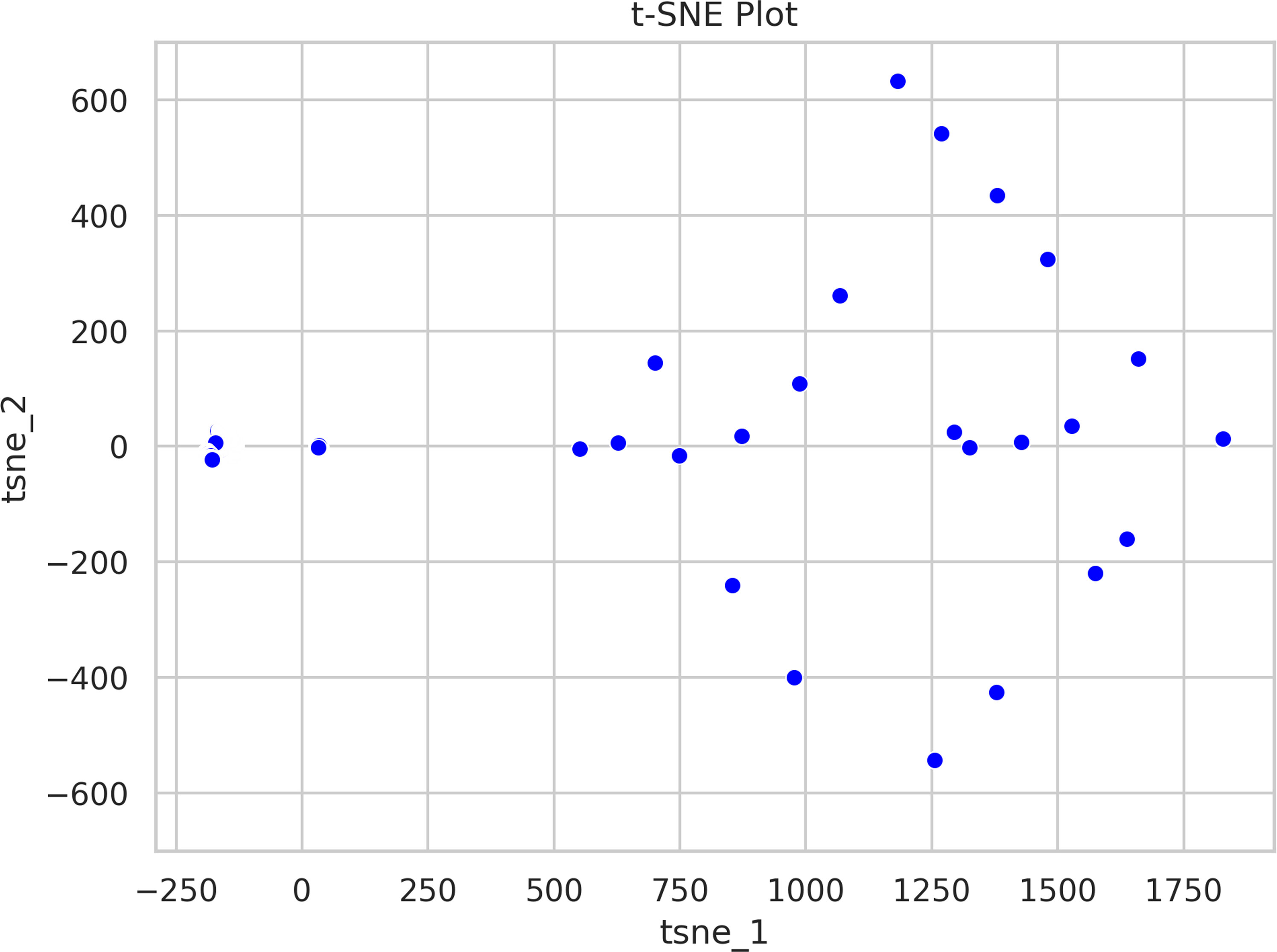
Two-dimensional representation of the original high-dimensional data. The t-distributed stochastic neighbor embedding (t-SNE) tries to preserve the original data’s local structure, so the close points remain close in this low-dimensional representation. The axis does not have a linear mapping to the features in the dataset.

Figure 10.

Since t-distributed stochastic neighbor embedding (t-SNE) tries to preserve the local structure of the original data, this figure shows that the generated (red) data points are close to the original ones.

Figures 9 and 10 lead us to hypothesize that the generated data is similar to the original data. To explore this, we analyzed the performance and accuracy of the model in the next section.

The performance of the proposed ctGAN model

In order to evaluate the quality of the data produced by a GAN, it is necessary to compare the distribution of the generated data with that of the original data. This comparison helps us to determine if the generated data shares any statistical characteristics with the original data, such as the shape of the distribution, the presence of outliers, and summary statistics like mean and variance.

One effective method for comparing the generated and original data distributions is through kernel density plots. A kernel density plot is a graphical representation of the probability density function of a continuous random variable. By overlaying the kernel density plot of the generated data on top of the original data plot, we can visually compare the two distributions and identify any discrepancies or differences.

Comparing the distributions of the generated and original data using kernel density plots can provide valuable insights into the quality of the generated data, as illustrated in Figures 11 to 16. These figures demonstrate the comparison of distributions for the signaling elements Ras, p21Cip1, mTOR, BCL, SNAIL, and TWIST.

Figure 11.

Distributions of the generated and original data using kernel density plots for the Ras signaling element.

Figure 12.

Distributions of the generated and original data using kernel density plots for the p21Cip1 signaling element.

Figure 13.

Distributions of the generated and original data using kernel density plots for the mTOR signaling element.

Figure 14.

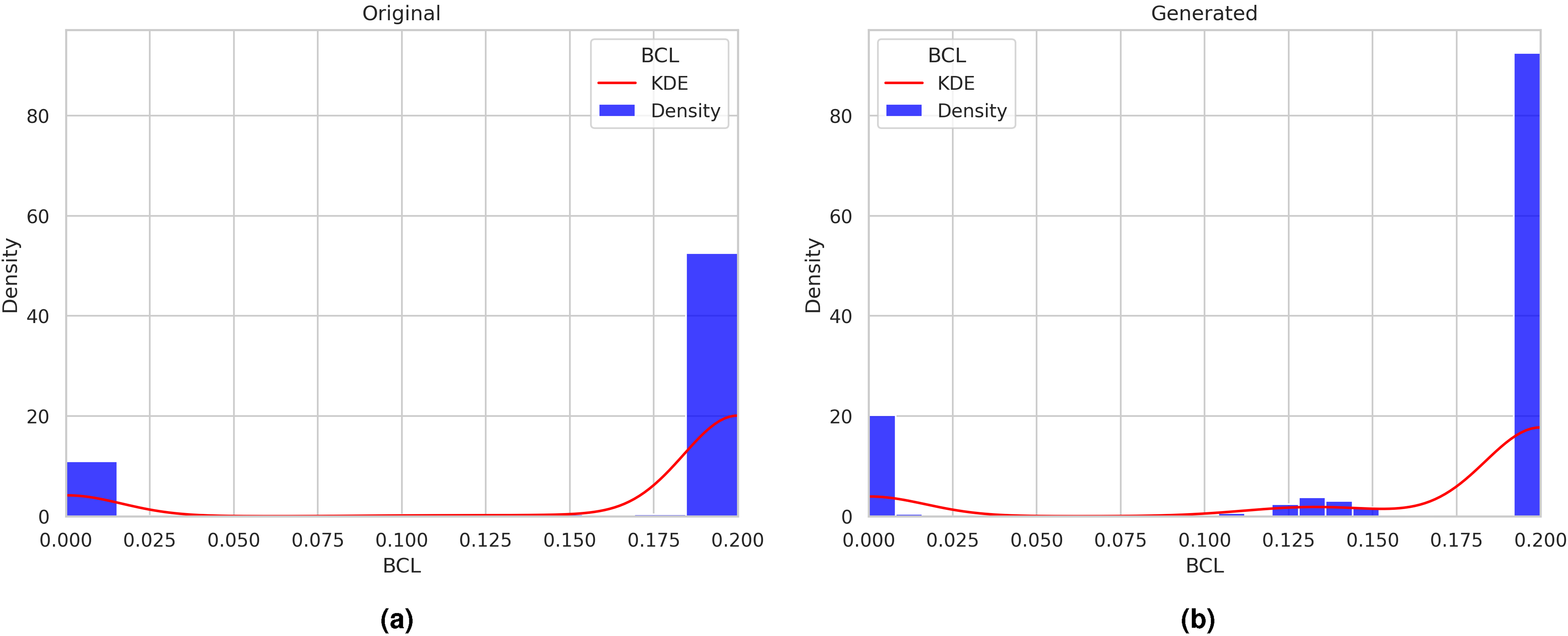
Distributions of the generated and original data using kernel density plots for the BCL signaling element.

Figure 15.

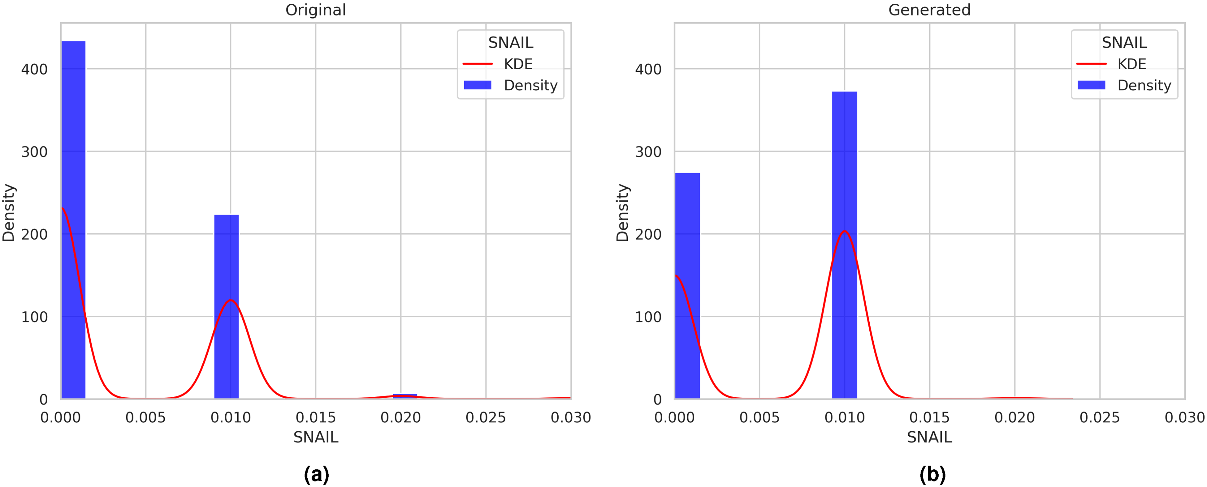
Distributions of the generated and original data using kernel density plots for the SNAIL signaling element.

Figure 16.

Distributions of the generated and original data using kernel density plots for the TWIST signaling element.

It is important to note that in Figures 11 to 16, the $X$ -axis represents the range of concentration values covered by the particular signaling element, while the $Y$ -axis indicates the density or number of activation patterns (dataset records) in which the signaling element reaches the same concentration value. As an example, lets consider Figure 11, which corresponds to the original (11(a)) and generated (11(b)) data distributions of the Ras signaling element. As shown in Figure 11(a), the concentration values characterizing the Ras signaling element in the original data ranges between 0.0 and 0.9, with specific values of 0.0, 0.2, and 0.7 to 0.9.

On the other hand, as illustrated in Figure 11(b), the concentration values generated by the ctGAN model for this signaling element precisely match the concentration values exhibited by the original data. This visual analysis can be extended to the distributions of signaling elements shown in Figures 12 to 16.

An alternative method for assessing the accuracy of the ctGAN model involves comparing the synthetic data with the real data using the EMD, a metric presented in Table 3. The EMD, also known as the Wasserstein or KR distance, is a measure of the distance between two probability distributions. It is calculated as the minimum amount of “work” required to transform one distribution into the other, where the work is defined as the amount of mass that needs to be moved multiplied by the distance it needs to be moved. This metric is particularly useful for comparing distributions that have multiple modes, a common feature of our dataset, as seen in Figures 11 to 16.

Table 3.

Wasserstein metric between each feature original data (signaling element) and its generated counterpart for the signaling elements shown in Figures 11 to 16.

Signaling element	Wasserstein metric
Ras	0.1718
mTOR	0.1382
p21Cip1	0.0346
BCL	0.0194
SNAIL	0.0033
TWIST	0.0008

The Wasserstein metric is a well-suited metric for various applications due to its important properties, such as non-negativity, symmetry, and triangle inequality. By using this metric, we can quantitatively evaluate the similarity between the synthetic and real data distributions. This allows us to determine if the ctGAN model has successfully captured the statistical characteristics of the original data distribution.

Since the Wasserstein metric serves as a measure of the “distance” between two probability distributions, a smaller value indicates a closer resemblance between the two distributions with regard to their mass distribution. To illustrate this point, we can examine the TWIST signaling element, which has a value of 0.0008 in Table 3. By comparing the histograms of the original and generated data in subfigures 16(a) and (b) of Figure 16, we observe that these two distributions have almost identical modes at around 0.0 and 0.01. This implies that the two distributions are similar in shape and support, or they have a similar mass concentration in different regions. When the two distributions are similar, only a small amount of work is required to transform one distribution into the other, resulting in a small distance value.

On the other hand, a larger value of the Wasserstein metric indicates a significant difference between the two distributions, requiring a considerable amount of work to be transformed into each other. For instance, consider the signaling element Ras in Table 3, which has a value of 0.1718 and whose distributions of the generated and original data are shown in Figure 11. Comparing subfigures 11(a) and (b), we can observe that, despite the general likeness, the distribution of the generated data (11(b)) has different modes, especially the mode in 0.9, which is different in the original data distribution (11(a)) that has modes in 0.7 and 0.9. This happens when the two distributions have different shapes, thus having a higher mass concentration in some regions than others. In this case, much work is necessary to transport mass from one distribution to another.

Comparative analysis of the accuracy of the supervised classification on both scenarios: Imbalanced dataset vs. balanced dataset

To evaluate the quality of the generated data, we measure the accuracy of the k-nn algorithm over the original and the generated data. The k-nn model is based on the idea that the class label of a given sample can be determined by finding the “k” closest samples in the training data and then choosing the majority class among them as the predicted class label. For this experiment, the model’s hyperparameters are $k=1$ nearest neighbor, Euclidean distance, 67% of the data for the training partition, and 33% for the test partition. The confusion matrices for original test data and augmented test data (original data plus generated date) are shown in Figure 17.

Figure 17.

Here, the confusion matrices for the original and augmented datasets are presented. The minor differences in the number of examples in each class are due to the random initialization of the train/test split, given that class 3 now has 634 more examples.

The initial accuracy of the k-NN model for the original test data is 99.59%, as seen in the confusion matrix in Figure 17(a). The supervised classification for class number 3, which is the class of interest, has correctly classified six instances out of eight, giving an accuracy of only 75%. On the other hand, the accuracy for the augmented data (original+generated) is lower, 99.36%, but the correctly classified instances for class number 3 are 220. In contrast, only one was incorrectly classified, giving an improved accuracy of 99.5%. This accuracy is the one that matters to us since we are only evaluating the quality of the data generated by the ctGAN.

Conclusions

In this study, we provided a machine learning-based strategy to correct the class imbalance in a cancer cell signaling dataset before using it in further supervised learning tasks. Specifically, in the approach proposed here, we generated additional instances for the minority class using a GAN, simulating the oversampling methodology. We aimed to determine how much the class balancing based on the GAN approach may increase the accuracy of supervised machine learning classification. The key findings from this work are outlined below:

Class imbalance in the cancer cell signaling dataset was solved using the ctGAN model to create new instances of the minority class (class 3), which only comprised 1% of the dataset’s total instances. This class number 3 represented 3.3% of the majority class (class 1). As a result, 634 new examples were generated for the minority class (class 3).

By contrasting the distributions of the generated data with the original data, the accuracy of the proposed ctGAN model was validated. This comparison allowed us to assess whether the created data’s statistical characteristics were similar to those of the original data. The comparison of distributions was carried out through two approaches: the kernel density plots and the Wasserstein metric.

In order to check how much the resulting class balance contributed to improving the accuracy of the supervised classification, we then applied supervised machine learning techniques to the balanced cell signaling dataset. The results revealed a 24.5% improvement in classification accuracy for patterns belonging to the minority class.

Our future work aims to conduct a comprehensive comparative analysis between ctGAN and the SMOTE ¹⁸ in addressing the class imbalance problem. Specifically, we plan to evaluate the effectiveness of ctGAN and SMOTE in creating synthetic samples of the minority class and improving the performance of machine learning models in classifying imbalanced datasets. The results will be analyzed to determine the effectiveness of ctGAN and SMOTE in improving the performance of machine learning models on datasets with varying degrees of class imbalance, which is a critical issue in various domains, including healthcare, finance, and cybersecurity.