Sage Journals: Discover world-class research

Abstract

This article proposes a hybrid susceptible–infected–removed model which takes into consideration the spatiotemporal dynamics of the individuals. The model is based on a system of discrete stochastic diffusion equations. To build these equations, the two-dimensional diffusion equations coming from a balanced method are coupled with the human displacement probability law pattern through a discretization made by the finite volume method for complex geometries. The validation of this model is applied to COVID-19 spread. Since it is actual and the statistics are available elsewhere. The case of a developed country is used for simulation under some assumptions. Firstly to fit the chosen displacement pattern, then the accuracy of the statistics provided helps to analyze the sensitivity of the parameters of the model. The results explain the influence of the population movement on the evolution of the spread.

Keywords

Discretization hybrid susceptible–infected–removed individual dynamics prediction model probability law pattern

Introduction

The evolution of transportation nowadays and confinement as a restriction measure during the COVID-19 pandemic show that the displacement of individuals is a key factor in the evolution of a spread. Many researchers in the mathematical field and beyond have proposed epidemiological models increasingly suitable for the study of the evolution of epidemics such as coronavirus, for the setup of the best strategies for the control of spread. Most of the proposed models are rooted in the compartmental epidemiological modeling proposed by Kermack and McKendrick^1,2 based on the systems of ordinary differential equations (ODEs), which describe only the temporal evolution of the spread.^3–10 Another class of models is the dynamical epidemic model called susceptible–infected–removed (SIR) model¹³ and its variants such as susceptible–exposed–infected–recovered (SEIR) and SIS. These later models are based on dividing the host population into a small number of compartments, each containing individuals that are identical in terms of their status with respect to the disease in question.¹⁴ Despite mathematical modeling having gained more scientific attention and awareness in epidemiology and medical science in general,^11,12 one notes that, in general, the spatial dynamic aspect of hosts is not explicitly highlighted in epidemiological studies.

Within the framework of prediction models, some studies focus on the estimation of the basic reproduction number $R_{0}$ based on the available data from the official statistics.^15,16 Others focus on the variation over time of the coefficients (the infection rate and the removal rate) in the SIR model.^17,18 Despite these developments, decision-makers find a lot of difficulties to take timely actions, due to the complexity of the epidemics, the non-homogeneous configuration of the population, and their movement. Some research had already pointed out this factor.^10,19 Wu¹⁹ built a model for the spatial spreading of diseases involving hosts in random displacement during certain stages of the progression of the disease. It led to a diffusion model based on the conservation law and Fick's law. The model is applied to the study of two cases of diseases namely the spread of rabies in continental Europe during the period 1945–1985 and the rate of West Nile virus spread in North America. Brockmann et al.¹⁰ noticed that in population dynamical systems, the diffusive dispersal is quite frequently combined with a reaction kinetic scheme which accounts for local interactions between various types of reacting agents. Sometimes groups of individuals of a single species that interact are classified according to some criteria. For instance, in the context of epidemic modeling, a population is often classified according to its infective status. In an approximation that neglects the intrinsic fluctuations of the reaction kinetics, one obtains for these systems reaction-diffusion equations.

Many authors have recently extended the SIR model to capture the spatiotemporal dynamics of individuals (see Gatto et al.,²⁰ Qianyue et al.,²¹ Giannone et al.,²² Chen et al.²³ and the references therein). Gatto et al.²⁰ examined the effects of prompted drastic measures for transmission containment in Italy. Based on modeling, they estimated the parameters of a meta-community SEIR-like transmission model that includes a network of 107 provinces connected by mobility at high resolution. Chen and co-authors²¹ built a data-driven epidemic simulator with COVID-19-specific features, which incorporated real-world mobility data capturing the heterogeneity in urban environments. Giannone et al.²² studied the effect of the economic exchange of populations due to their displacements, the economic impact, and possible optimization of management policies for the conservation of the economy and the reduction of loss of human life between the states of the US. Chen et al.²³ introduced a new model which incorporated asymptomatic infections and population migration into SEIR, hence, referred to as the SEIAR (susceptible-exposed-infected-asymptomatic-recovered) model with population migration. However, in all these approaches, there's no concrete modeling of the random aspect of the movement of individuals coupled with the impact of administrative divisions.

The purpose of this study is to build a hybrid SIR model named SIR-D which combines the traditional SIR with a stochastic diffusion term that represents the random spatiotemporal dynamics of individuals. The approach sets certain hypotheses which, on the one hand, consider the random aspect of the dynamic of individuals and, on the other hand, takes into account geographical conditions like administrative divisions. The motivation comes from the fact that the forecasts made by the statistics are not always representative due to the complexity of human interactions and geographical conditions.²⁰ To integrate the random aspect in the proposed model, we gained inspiration from existing studies relating to the development of human mobility patterns.^10,24 This extension is possible for any variant of the SIR model (SIS, SEIR, SEAIR, etc.) and other phenomena which involve the movement of the hosts during their evolution.

According to Currie et al.²⁵ who stated that simulation modeling can help to support decision-makers in making the most informed decision, this work is a precursor to the design of a decision support system that will allow the decision-maker to simulate the evolution of an epidemic according to the displacement profile of a population in order to make the right decision. In this regard, the case of the COVID-19 pandemic is used to validate the proposed model. The simulation is done on a selected country that fits with the hypothesis of probability law's pattern and the results are confronted with the existing statistics data coming from www.kaggle.com. The formulation of the model uses the 2D diffusion equation. For numerical resolution, a discretization is made using the finite volume method for complex geometries to capture administrative divisions. A GIS software was subsequently used to extract the spatial data used as input in our model. Data retrieved are processed using algorithms and data science techniques found by Igual and Segui²⁶ and implemented in the Python environment to numerically solve the system of equations obtained. The simulation results are presented alongside the trend of the true data as a way of validating assumptions on the input parameters.

The remainder of this paper is structured as follows: the “Model formulation and assumptions” section presents our methodology, focusing on the manner in which the model is built with finite volume discretization for complex geometries and diffusion matrix structure to obtain a hybrid SIR. The “Simulation and validation” section describes the application of the model to the COVID-19 data from Italy. The “Conclusion” section gives some concluding remarks and the direction of further works.

Model formulation and assumptions

Background

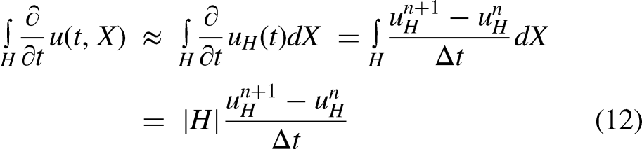
The general form of the equation modeling the evolution of mobile entities that interact with each other is given by:

\frac{\partial}{\partial t} u (t, x, y) = Q (u (t, x, y)) + f (x, y, u (t, x, y)), t > 0, (x, y) \in R^{2}

(1)

Similar equations come up in a wide variety of fields such as combustion, chemistry, biology, or ecology.²⁷ Applied to the population dynamics, the quantity u (t, x, y) represents the population density at time t at the position (x, y). The reaction term f (x, y, u) corresponds to the growth rate of the population. The movement of individuals is described by the dispersion operator

Q

. Depending on the individual movement mode, the operator

Q

is local or non-local.

Our attention is focused mainly on a single type of reaction–diffusion equation where the dispersion operator $Q = D (\frac{\partial^{2}}{\partial x^{2}} + \frac{\partial^{2}}{\partial y^{2}})$ is a second-order elliptic differential operator and D is the diffusion coefficient, hence

\begin{aligned} \frac{\partial}{\partial t} u (t, x, y) = & D [\frac{\partial^{2}}{\partial x^{2}} u (t, x, y) + \frac{\partial^{2}}{\partial y^{2}} u (t, x, y)] \\ + f (x, y, u (t, x, y)) \\ f o r t > 0 (x, y) \in R_{+}^{2} \end{aligned}

(2)

In the same way with a balance sheet approach in control volume that originates from particles diffusion, one obtains the following equation:

\begin{aligned} \frac{\partial}{\partial t} u (t, x, y) = D (\frac{\partial^{2}}{\partial x^{2}} u (t, x, y) + \frac{\partial^{2}}{\partial y^{2}} u (t, x, y)), \\ f o r t > 0, (x, y) \in R^{2} \end{aligned}

(3)

which is the basic material for our modeling.²⁸

Contextualization and meshing

A finite volume scheme on unstructured staggered grids

The finite volume scheme is found by integrating the Stokes problem²⁹ or Laplace problem³⁰ on a control volume of a discretization mesh and finding an approximation of the fluxes on the control volume boundary in terms of the discrete unknowns.

To give the assumptions needed on the mesh, we consider here the Laplace problem in an open bounded polygonal subset $Ω \subset R^{d}$ , (d = 2 or 3) with Dirichlet boundary condition

- \nabla^{2} u (X) = f (X) \forall X \in Ω

(4)

u (X) = 0 \forall X \in \partial Ω

where f is a function defined from Ω into

R

. Let Ω

\subset R^{2}

, T be an admissible finite volume mesh of Ω and K an element in T. By integrating the above Laplace equation over K, one obtains:

\int_{K} - \nabla^{2} u d X = \int_{K} f d X \forall X \in Ω

(5)

By Stokes’ formula, we can rewrite this equation as follows:

- \int_{\partial K} \nabla u . n_{K} (X) d_{γ} (X) = \int_{K} f (X) d X \forall X \in Ω

(6)

where

d_{γ} (X)

denotes the integral with respect to the one-dimensional measure on the edge of Ω, and

n_{K}

is the outward unit normal to

\partial K

, the boundary of K. As K is polygonal, we can decompose ∂K into n edges

σ_{i}, i = 1, \dots, n

, each of length

| σ_{i} |

, while

E_{K} = {σ_{1}, \dots, σ_{n}}

is the set of edges. Hence, we have

- \sum_{σ_{i} \in E_{K}} \int_{σ_{i}} \nabla u . n_{K, σ_{i}} d_{γ} (X) = \int_{K} f (X) d X

(7)

where

n_{K, σ_{i}}

is the outward unit normal to

σ_{i}

. We now seek to approximate

\nabla u . n_{K, σ_{i}}

in a consistent manner in every edge

σ_{i}

. For any (K, L)

\in T^{2}

with

K \neq L

, the d-dimensional Lebesgue measure of

K \cap L

is either 0 or

σ_{i} f o r σ_{i} \in E_{K}

. Consider the discrete unknowns

(u_{K})_{K \in T}

, an approximation of

u (X_{K})

. For an edge

σ_{i} = K | L

, it is assumed that

X_{K} \neq X_{L}

and that the straight line

d_{K, L}

going through

X_{K}

and

X_{L}

is orthogonal to K|L. The term

\nabla u . n_{K, σ_{i}}

can then be approximated by the expression

\frac{u (X_{L}) - u (X_{K})}{d_{K, L}}

Given that

| σ_{i} |

is the length of edge

σ_{i}

, the integral

\int_{σ_{i}} \nabla u \cdot n_{k} d_{γ}

can be approximated by

\int_{σ_{i}} \nabla u . n_{k} d_{γ} \approx F_{K, σ_{i}} = | σ_{i} | \frac{u_{L} - u_{K}}{d_{K, L}}

(8)

for

σ_{i} \in E_{K}

and

K \in T

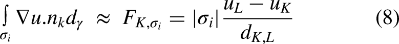
The finite volume scheme is, therefore, written

\sum_{σ_{i} \in E_{K}} F_{K, σ_{i}} = | K | f_{K}

(9)

where

| K |

is the measurement of K and

f_{K} = \frac{1}{| K |} \int_{K} f (X) d X

Under boundary conditions, each $F_{K, σ_{i}}$ can be defined as

F_{K, σ_{i}} = {\begin{matrix} - | σ_{i} | \frac{u_{L} - u_{K}}{d_{K, L}} i f σ_{i} = K | L \\ - | σ_{i} | \frac{u_{K}}{d_{K, σ_{i}}} i f σ_{i} \subset \partial Ω a n d σ_{i} \in E_{K} \end{matrix}

(10)

where

d_{K, σ_{i}}

is the distance between

X_{K}

and the edge

σ_{i}

Contextualization and meshing

Let Ω be a bounded open set of $R^{2}$ (represented by these sample regions as shown in Figure 1) and T is an admissible finite volume mesh of Ω (represented by these sampled regions and approximated by polygons as shown in Figure 2). We recall that this is just for illustration as the real scheme will be done with the help of geographic information system tools. We will let H $\in$ T.

Figure 1.

The selected regions.

Figure 2.

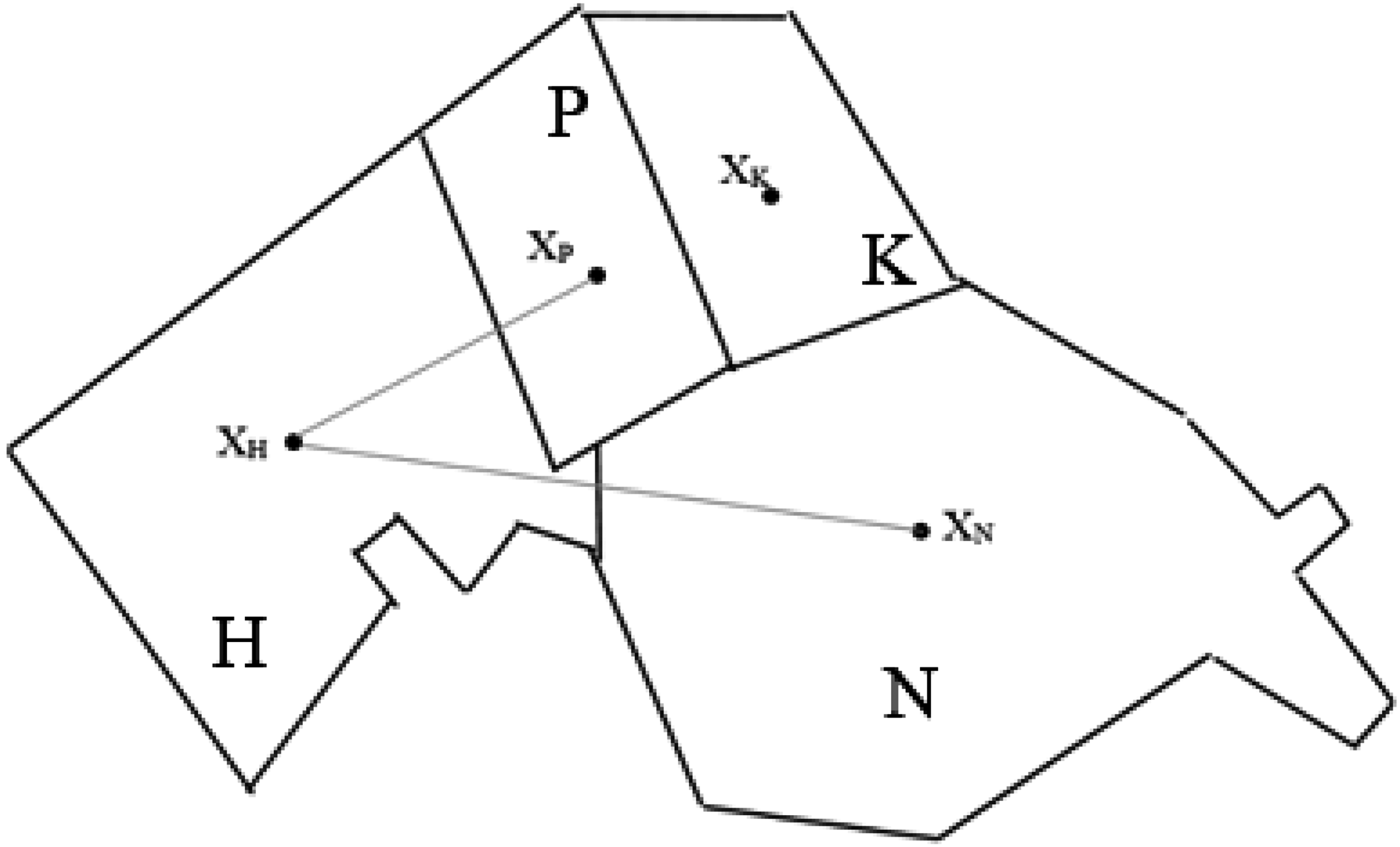
Polygonal approximation of four regions.

Henceforth, we will consider:

X_H $(x_{H}, y_{H})$ to be the centroid position of mesh H,

X_P $(x_{P}, y_{P})$ the centroid position of the mesh P,

X_N $(x_{N}, y_{N})$ the centroid position of the mesh N,

X_K $(x_{K}, y_{K})$ the centroid position of the mesh K,

$| σ_{H N} |$ is the measure of edge $σ_{H N} = H | N$ , assuming that $X_{H} \neq X_{N}$ and that the straight line $d_{H, N}$ going through $X_{H}$ and $X_{H}$ is orthogonal to H|N as in the “A finite volume scheme on unstructured staggered grids” section

$| σ_{H P} |$ is the measure of edge $σ_{H P} = H | P$ , assuming that $X_{H} \neq X_{P}$ and that the straight line $d_{H, P}$ going through $X_{H}$ and $X_{P}$ is orthogonal to H|P as in the “A finite volume scheme on unstructured staggered grids” section

$| H |$ is the measurement of the surface area H defined by $| H | \equiv \int_{H} d x d y \equiv \int_{- \infty}^{+ \infty} \int_{- \infty}^{+ \infty} ‖ {(x, y) \in H} d x d y$ ,

$d_{H N}$ = ||X_H – X_N||₂ = $[{(x_{H} - x_{N})}^{2} + {(y_{H} - y_{N})}^{2}]^{\frac{1}{2}}$ is the distance between X_H and X_N,

$\partial H$ is a set of all boundaries of domain H.

The quantity $\frac{\partial}{\partial t} u (t, X)$ will be approached using Euler's explicit method:

\frac{\partial}{\partial t} u (t, X) \approx \frac{u^{n + 1} - u^{n}}{Δ t}

(11)

where

u^{n + 1}

represents the number of mobile entities in the site at time t + dt,

u^{n}

its value at the time t, and

X = (x, y)

. We will assume that

u (t, X)

is constant in mesh H at any given moment, hence, we have

u (t, X) \approx u (t, X_{H}) = u_{H} (t)

. Then the following approximation can then be made:

\int_{H} \frac{\partial}{\partial t} u (t, X) \approx \int_{H} \frac{\partial}{\partial t} u_{H} (t) d X = \int_{H} \frac{u_{H}^{n + 1} - u_{H}^{n}}{Δ t} d X = | H | \frac{u_{H}^{n + 1} - u_{H}^{n}}{Δ t}

(12)

With the finite volume scheme above,¹⁰ the term $\int_{H} \nabla^{2} u (t, X) d X$ is transformed following Stokes’ formula to $\int_{\partial H} \nabla u \cdot n_{K} (X) d_{γ} (X)$ . In the same way, as in the “A finite volume scheme on unstructured staggered grids” section, the finite volume method applied to the basic equation in the area of the mesh H leads to

\int_{H} \frac{\partial}{\partial t} u (t, X) d X = \int_{H} D \nabla^{2} u (t, X) \leftrightarrow \int_{H} \frac{\partial}{\partial t} u_{H} (t) d X = D \int_{H} \nabla u (t, X) \cdot n_{K} (X) d_{γ} (X)

(13)

With the above considerations applied to,¹⁴ one obtains the following finite volume scheme

| H | \frac{u_{H}^{n + 1} - u_{H}^{n}}{Δ t} = D_{N H} | σ_{H N} | \frac{u_{N}^{n} - u_{H}^{n}}{d_{H N}} + D_{P H} | σ_{P H} | \frac{u_{P}^{n} - u_{H}^{n}}{d_{H P}}

(14)

u_{H}^{n + 1} = D_{N H} | σ_{H N} | Δ t \frac{u_{N}^{n} - u_{H}^{n}}{| H | d_{H N}} + D_{P H} | σ_{P H} | Δ t \frac{u_{P}^{n} - u_{H}^{n}}{| H | d_{H P}} + u_{H}^{n}

(15)

where

$u_{H}^{n + 1}$ represents the number of mobile entities at the time t + dt in H

$D_{N, H}$ and $D_{P, H}$ represent two elements of the diffusion matrix D.

Because of meshing, D is no longer a simple coefficient but a diffusion matrix depending on individual movement from one mesh to another. Recall the general form

D = ω P

(16)

where

ω

represents the average speed of individual diffusion and P is the matrix of random contributions given in the “Definition of the diffusion matrix D” section.

So $D_{N, H} = ω P_{N, H}$ ; $P_{N, H}$ is the probability of moving from mesh N to H estimated by the probability law pattern that fits with the movement. This is how we compute all the diffusions matrix elements.

$Δ t$ is the time step in the numerical scheme

Similarly, for the rest of the sites (P, N, K) we obtain the following equations:

Site P

u_{P}^{n + 1} = D_{H P} | σ_{P H} | Δ t \frac{u_{H}^{n} - u_{P}^{n}}{| P | d_{P H}} + D_{N P} | σ_{P N} | Δ t \frac{u_{N}^{n} - u_{P}^{n}}{| P | d_{P N}} + D_{K P} | σ_{P K} | Δ t \frac{u_{K}^{n} - u_{P}^{n}}{| P | d_{P K}} + u_{P}^{n}

(17)

Site N

u_{N}^{n + 1} = D_{H N} | σ_{N H} | Δ t \frac{u_{H}^{n} - u_{N}^{n}}{| N | d_{N H}} + D_{P N} | σ_{N P} | Δ t \frac{u_{P}^{n} - u_{N}^{n}}{| N | d_{N P}} + D_{K N} | σ_{N K} | Δ t \frac{u_{K}^{n} - u_{N}^{n}}{| N | d_{N K}} + u_{N}^{n}

(18)

Site K

u_{K}^{n + 1} = D_{P K} | σ_{K P} | Δ t \frac{u_{P}^{n} - u_{K}^{n}}{| K | d_{K P}} + D_{N K} | σ_{K N} | Δ t \frac{u_{N}^{n} - u_{K}^{n}}{| K | d_{P N}} + u_{K}^{n}

(19)

Boundary conditions are implicitly considered because the quantities above are zero everywhere else except on the boundaries between our experimental environments.

For a general formulation for any mesh H, we can write the numerical scheme as follows:

u_{H}^{n + 1} = \sum_{N \in n e i g h b o r (H)} D_{N, H} | σ_{H N} | Δ t \frac{u_{N}^{n} - u_{H}^{n}}{| H | d_{H N}} + u_{H}^{n}

(20)

$u_{H}^{n + 1}$ represents the number of mobile entities at the time t + dt in H

$D_{N, H}$ represents an element of the diffusion matrix $D_{i, j}$

$| σ_{H, N} |$ represents the length of the border between

|H| represents the area of H

$d_{H, N}$ represents the distance between the two centroids H and N

Definition of the diffusion matrix $D$

The diffusion part of the basic equation is related to the human displacement which is random and complex. Thus it requires complementary effort to its formulation. That is why we find in the literature the relevant studies on this topic independently of the discipline. In physics, random walk processes with a power-law single-step distribution are known as Lévy flights;^31,32 Lévy flights are qualitatively different from ordinary random walks. Another study in telecommunications used subscribers' telephone data to estimate human mobility in developed countries (24).^33,34 According to their thinking, the pervasive usage and the high penetration rates of mobile phones have made mobile network data the largest mobility data source ever. Many other theories are used to explain human displacement as the trajectory distance, also called jump length, which corresponds to the traveled distance during a trip. Brockmann et al.¹⁰ state that the jump length Δr follows a power-law distribution:

P (Δ r) = Δ r^{- (1 + β)}

(21)

where β < 2. This finding reveals that people usually have short-length trips and fewer long-distance travels. In 2008, the jump length was described as following a truncated power-law distribution³⁵

p (Δ r) \sim (Δ r + Δ r_{0})^{- β} \exp (\frac{Δ r}{k})

(22)

with β = 1.75 ± 0.15, Δr0 = 1.5 km, and k is a cut-off value depending on the dataset.

Based on the above observation, we will build the diffusion matrix D which will be composed of two terms; an average diffusion speed, and a probabilistic displacement matrix between regions. The computation of the coefficients of the probability matrix is based on humans’ movement probability law pattern. There are several displacement patterns in the literature depending on the context of the study. In general, we will have

D = ω p

In the above formula,

ω

is the average diffusion speeds and P the probability matrix.

ω

is estimated as follows

ω = \frac{σ^{2}}{Δ t}

, where σ is the standard deviation between all inter-region travel distances and, Δt the characteristic time step.¹⁰ The construction of the probability matrix p is as follows:

Let $Ω$ be a physical space and $P_{Ω}^{t} = {A_{1}, A_{2}, \dots, A_{n}}$ a spatial partition of $Ω$ at a given time t. Each $A_{i} \in P_{Ω}^{t}$ has a number $n_{i}^{t}$ mobile entities at the time t. At a time $t + d t$ there is a random displacement between the $A_{i}$ thus modifying all the $n_{i}^{t} cardinals$ , which become $n_{i}^{t + d t}$ depending on the various transitions. We thus obtain $P_{Ω}^{t + d t} = {A_{1}^{'}, A_{2}^{'}, \dots, A_{n}^{'}}$ .

Here we are interested in the probability $p_{i, j}$ that an element $a \in A_{i}$ will be found in $A_{j}$ knowing of course that $A_{i} \cap A_{j} = \emptyset$ . At the time $t + d t$ , the transition $P_{Ω}^{t} \to P_{Ω}^{t + d t}$ allows us to construct the following probability matrix

p = (\begin{matrix} p_{11} & \dots & p_{1 n} \\ ⋮ & ⋱ & ⋮ \\ p_{n 1} & \dots & p_{n n} \end{matrix})

Interpretation of de model applied to SIR

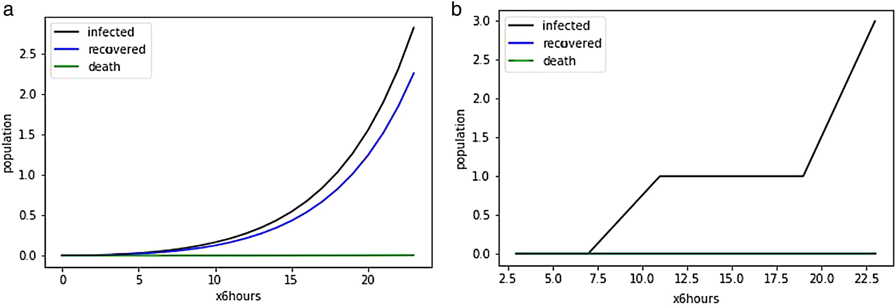
In the traditional SIR model, there are three compartments represented in Figure 3:

Susceptible: individuals who might become infected if exposed assuming that they have no immunity to the infectious agent.

Infectious: infected individuals who can transmit the infection to susceptible individuals that they contact.

Removed: individuals recovered from the disease.

Figure 3.

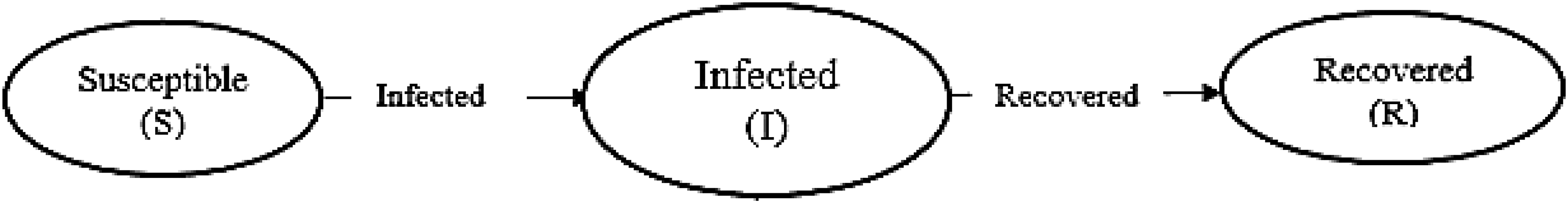
State chart of the dynamic of susceptible–infected–removed (SIR).

The transitions between states are interpreted as follows:

{\begin{matrix} \frac{d S (t)}{d t} = - β \frac{S I}{N} \\ \frac{d I (t)}{d t} = β \frac{S I}{N} - α I - γ I \\ \frac{d R (t)}{d t} = α I \end{matrix}

(23)

Taking into account the movement of individuals in their environment, the explicit incorporation of spatial spreading may yield important insights into the dynamics of interacting individuals. This is made by adding the diffusive term developed above that increases the precision of the model. One obtains the hybrid form given below:

{\begin{matrix} \frac{d S (t)}{d t} = - β \frac{S I}{N} + D \nabla^{2} S \\ \frac{d I (t)}{d t} = β \frac{S I}{N} - α I - γ I + D \nabla^{2} I \\ \frac{d R (t)}{d t} = α I + D \nabla^{2} R \end{matrix}

(24)

where D is the diffusion coefficient; t is the time; β is the infection rate; α is the removal rate, and γ is the death rate. By substitution of (15) in the system, we obtain

{\begin{matrix} S_{H}^{n + 1} = - β Δ t (\frac{S_{H}^{n} * I_{H}^{n}}{N_{t o t, H}^{n}}) + \sum_{N \in n e i g h b o r (H)} D_{N, H} | σ_{H N} | Δ t \frac{S_{N}^{n} - S_{H}^{n}}{| H | d_{H N}} + S_{H}^{n} \\ I_{H}^{n + 1} = - Δ t (α I_{H}^{n} + γ I_{H}^{n}) + β Δ t (\frac{S_{H}^{n} * I_{H}^{n}}{N_{t o t, H}^{n}}) + \sum_{N \in n e i g h b o r (H)} D_{N, H} | σ_{H N} | Δ t \frac{I_{N}^{n} - I_{H}^{n}}{| H | d_{H N}} + I_{H}^{n} \\ R_{H}^{n + 1} = α Δ t I_{H}^{n} + \sum_{N \in n e i g h b o r (H)} D_{N, H} | σ_{H N} | Δ t \frac{R_{N}^{n} - R_{H}^{n}}{| H | d_{H N}} + R_{H}^{n} \end{matrix}

(25)

N_{t o t, H}^{n} = S_{H}^{n} + I_{H}^{n} + R_{H}^{n}

The resulting conservation equation in the form of a diffusion equation was developed in previous works.²⁸

Simulation and validation

Assuming that the mortality rate due to COVID-19 is not negligible, we add to the traditional SIR model a fourth state (death state) that takes into consideration the number of deaths due to the illness (Figure 4).

Figure 4.

State chart of the dynamic of susceptible–infected–removed (SIR).

This consideration modifies the equations system as follows:

{\begin{matrix} S_{H}^{n + 1} = - β Δ t (\frac{S_{H}^{n} * I_{H}^{n}}{N_{t o t, H}^{n}}) + \sum_{N \in n e i g h b o r (H)} D_{N, H} | σ_{H N} | Δ t \frac{S_{N}^{n} - S_{H}^{n}}{| H | d_{H N}} + S_{H}^{n} \\ I_{H}^{n + 1} = - Δ t (α I_{H}^{n} - γ I_{H}^{n}) + β Δ t (\frac{S_{H}^{n} * I_{H}^{n}}{N_{t o t, H}^{n}}) + \sum_{N \in n e i g h b o r (H)} D_{N, H} | σ_{H N} | Δ t \frac{I_{N}^{n} - I_{H}^{n}}{| H | d_{H N}} + I_{H}^{n} \\ R_{H}^{n + 1} = α Δ t I_{H}^{n} + \sum_{N \in n e i g h b o r (H)} D_{N, H} | σ_{H N} | Δ t \frac{R_{N}^{n} - R_{H}^{n}}{| H | d_{H N}} + R_{H}^{n} \end{matrix} a n d M_{H}^{n + 1} = γ I_{H}^{n} Δ t + M_{H}^{n}

(26)

Input data

The simulation is focused on Italy before confinement from 1 to 6 March 2020. The choice of Italy is motivated by two major reasons. First, because the probability law used was set up in the context of human interaction in developed countries, second, the availability and the accuracy of the official data related to the pandemic. The COVID-19 pandemic data used in this study come from the www.kaggle.com website where we extracted the dataset (Table 1). The map of Italy is extracted from Google Earth, and the demographic data are collected on Wikipedia. We used the ArcGIS software to compute the distance between the centroids of the regions and to approximate the perpendicular border length of the adjacent regions as in the “Contextualization and meshing” section

Table 1.

Pandemic input data for simulation.

Region	Recovered (R0)	Deaths M(0)	Total Positive Cases I(0)	Susceptible S(0)	Population N(0)
Abruzzo	0	0	5	1,322,755	1,322,760
Apulia	0	0	3	4,067,291	4,067,294
Basilicata	0	0	0	571,409	571,409
Calabria	0	0	1	1,966,648	1,966,649
Campagna	0	0	17	5,841,733	5,841,750
Emiliaromagna	0	8	285	4,446,636	4,446,929
Friuli	0	0	6	1,218,153	1,218,159
Lazio	3	0	6	5,891,536	5,891,545
Liguria	4	0	25	1,566,278	1,566,307
Lombardia	73	24	984	10,010,780	10,011,861
Marche	0	0	25	1,539,252	1,539,277
Molise	0	0	0	310,850	310,850
Piemonte	0	0	49	4,395,314	4,395,363
Sardegna	0	0	0	1,654,796	1,654,796
Sicily	2	0	9	5,057,236	5,057,247
Toscana	1	0	13	3,742,575	3,742,589
Trentino	0	0	0	1,061,046	1,061,046
Umbria	0	0	2	889,693	889,695
Valledaosta	0	0	0	126,832	126,832
Veneto	0	2	263	4,907,143	4,907,408

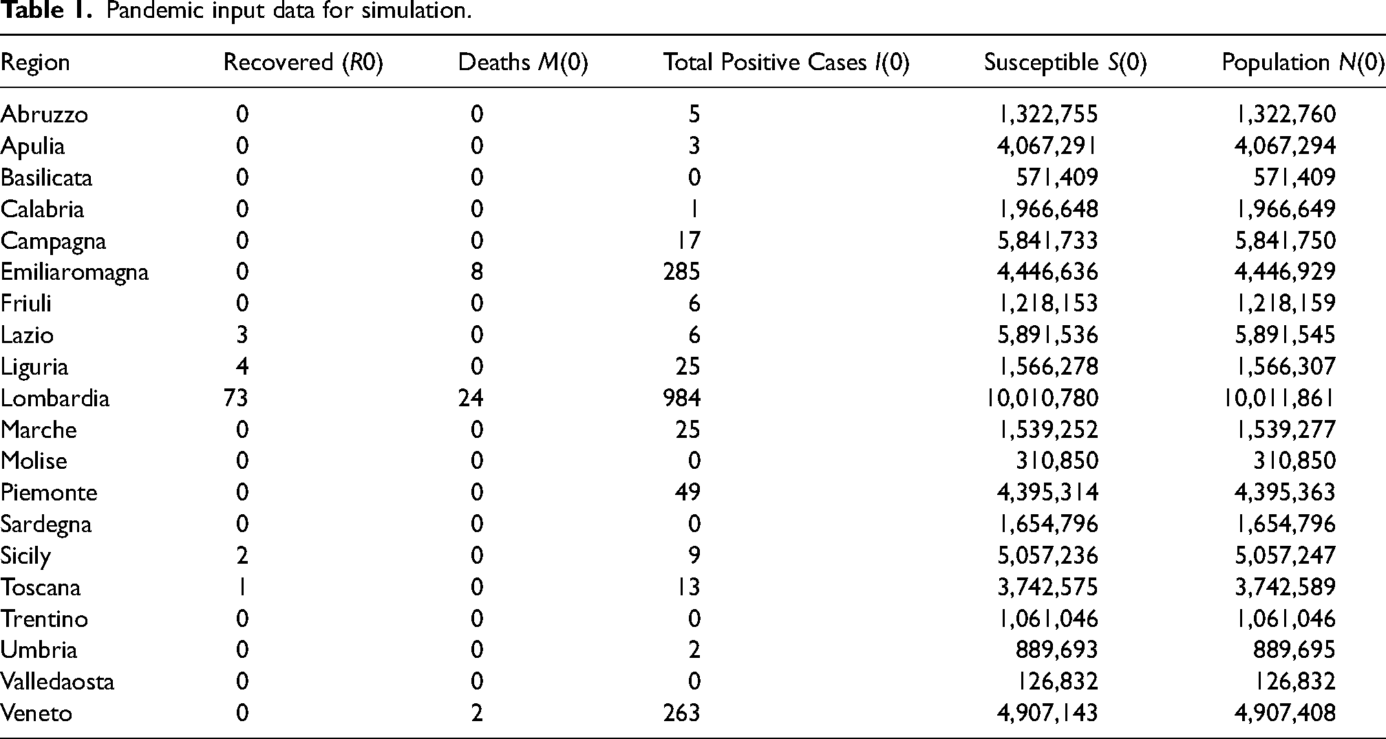
Figure 5 shows some discretization traces on the GIS software for the extraction of spatial data.

Figure 5.

Distance between centroids as spatial input data.

Table 1 gives the initial values used in the simulation (1 March 2020).

- N(0) = the total population in a region,

- S(0) = the number of people likely to be contaminated,

- I(0) = the number of positive cases on this date,

- R(0) = the number of cases healed on this date,

- M(0) = the number of deaths.

The population will be assumed to be homogeneous where everyone is likely to contract the disease. A short time interval is chosen for the simulation (1–6 March) due to the time-varying property of the rates of the SIR model. In the case of a simulation over a long period of time, it would be necessary to take into account these variations as a time function in the definition of the SIR model parameters. The infection rate (β), removal rate (α), and death rate (γ) are obtained empirically from the available official statistics (17).

- N = total human population in a given region

- I = total infected given by the test cases

- Ir = supposed total infected

- M = total death

- Rc = recovered by cure

- α = recovered rate by cure

- β = the infection rate

- γ = death rate

Ir = \frac{100 * I}{20} (80 % o f I r a r e a s y m p t o m a t i c s)

γ = \frac{M}{I r}, α = \frac{R_{c} + 0.8 * I_{r e a l}}{I_{r e a l}}, β = \frac{I_{r}}{N}

The adjustment of the coefficients α, β, and γ is mainly based on the number of deaths. This is true because all death causes are known (including the COVID-19 pandemic). The other data, namely the number of infected or recovered seem not representative because tests are generally performed on samples made up of suspicious people with a high body temperature, which is low compared to the real size of the population

N (t) = S (t) + I (t) + R (t) - M (t)

Table 2 gives the list of parameters which are time-based functions used in the equations. Their initial values are found in Table 1.

Table 2.

Model variables and parameters.

Values	Descriptions
N(t)	Total human population
S(t)	Population of susceptible humans
I(t)	Population of infected humans
R(t)	Population of recovered humans
M(t)	Population of dead humans

Simulation results

In every region, four discrete equations are computed. That makes a total of 80 equations by considering the 20 regions of Italy. The following figures present the result from some regions. The graphics at the left show the simulation of the pandemic, assuming that the entire population is susceptible and the graphics at the right are the representation of the statistical data collected during the same period.

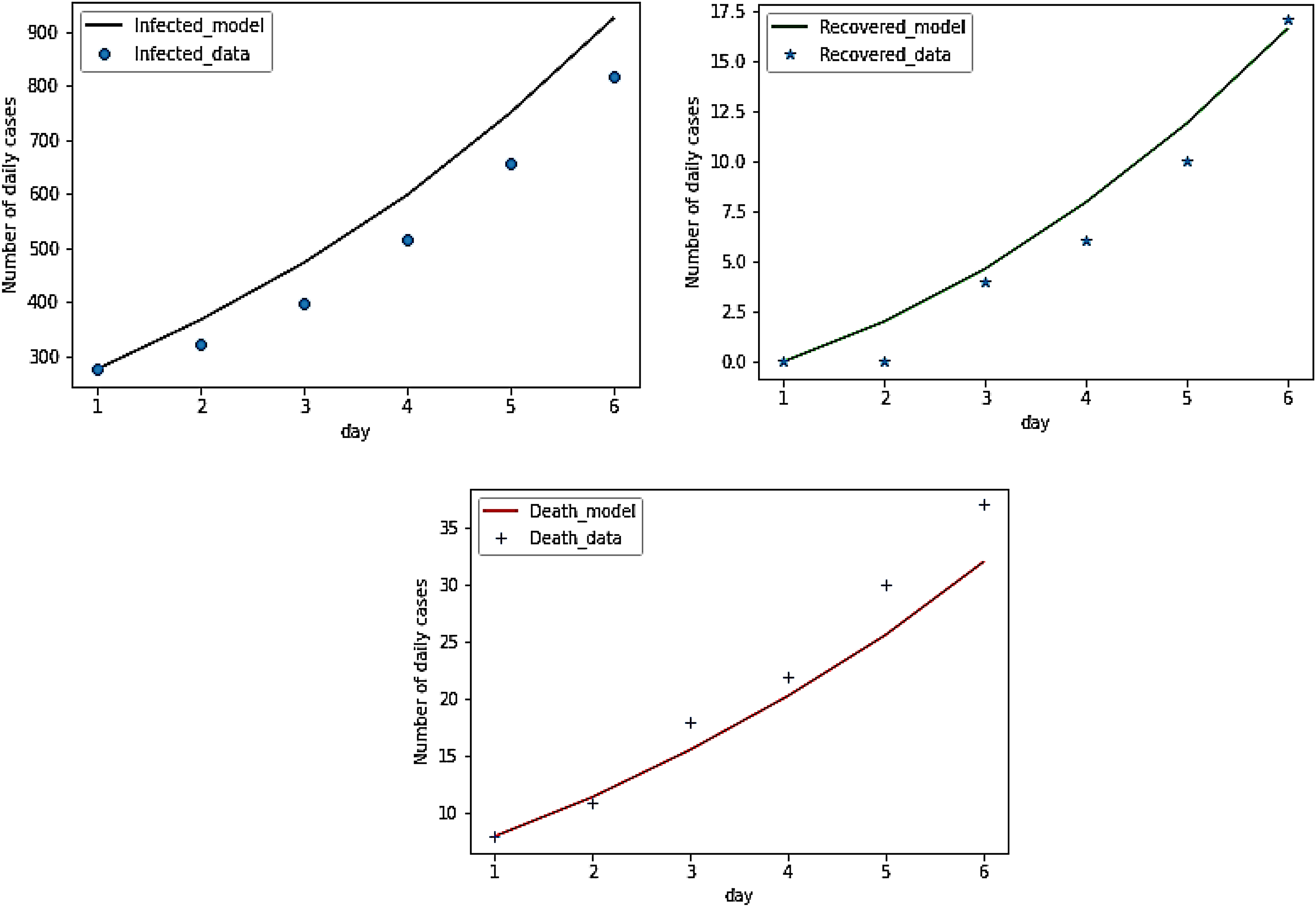
Figure 6(a) shows the evolution of the epidemic in the “Lombardia” region, assuming that the entire population is susceptible (10,011,861 people). Figure 6(b) is the visualization of the data for a sample of 13,556 tests performed until 6 March 2020.

Figure 6.

(a) Simulation in Lombardia and (b) statistics in Lombardia.

The statistical data shows that neighboring regions to Lombardia (“Emilia Romagna,” “Veneto,” and “Piemonte”) have a higher number of infected persons than others, this is because Lombardia was the most infected region. The results of our simulations fit with this reality given that our model considers the mixing of populations that share land borders. This statement is illustrated in the following diagrams.

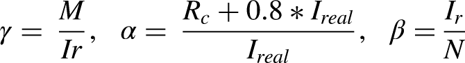
Figure 7(a) is the evolution of the disease in the entire population (4,446,929 people) given that everyone is a suspect and Figure 7(b) is the data visualization of data obtained for tests carried out on 3136 persons.

Figure 7.

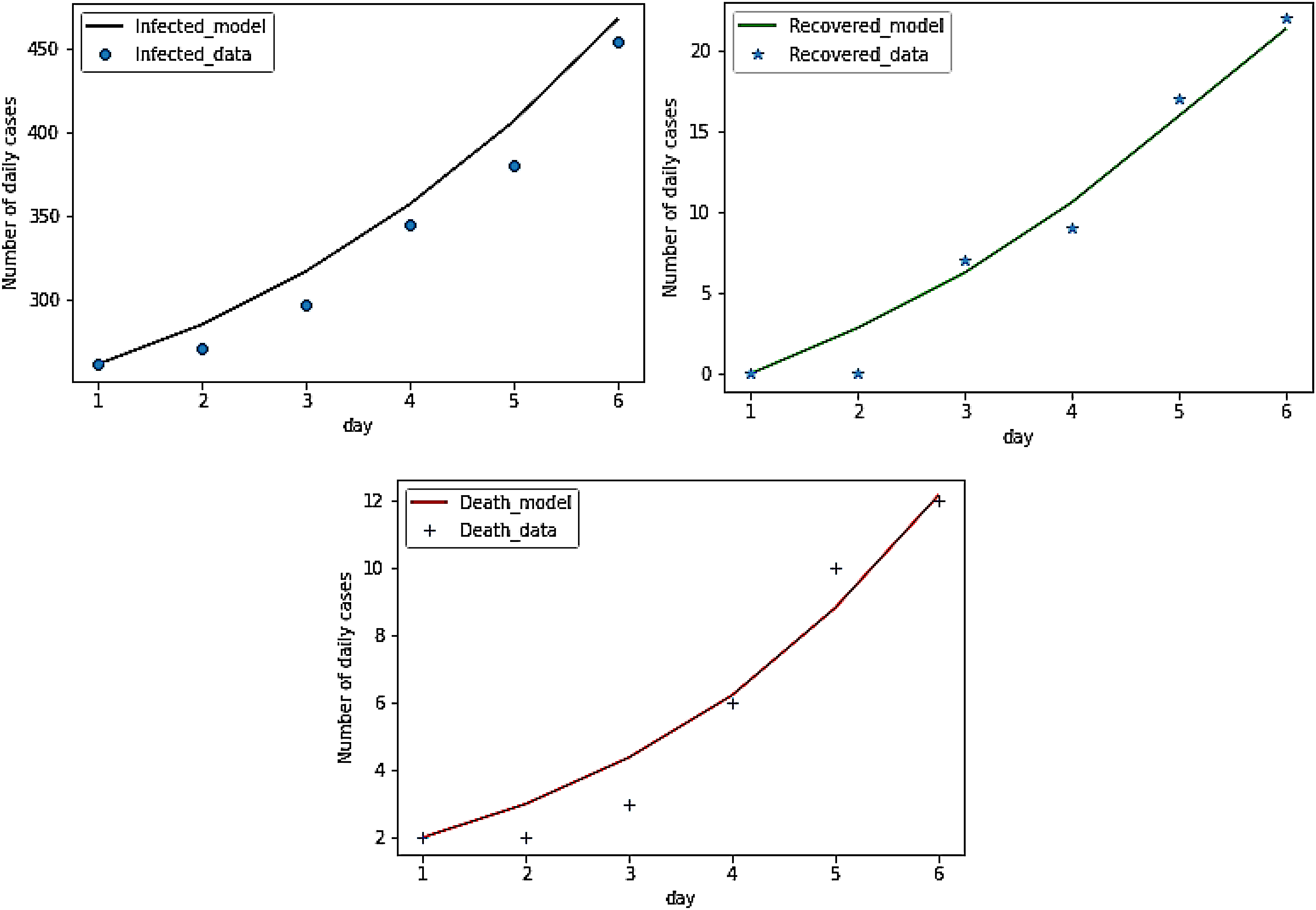
(a) Simulation in Emilia Romagna and (b) statistics in Emilia Romagna.

In line with what precedes, Figure 8(a) is the evolution of the disease in the entire population (4,907,408) and Figure 8(b) is the visualization of data for tests carried out on 13,023 persons.

Figure 8.

(a) Simulation in Veneto and (b) statistics in Veneto.

Figure 9(a) is the evolution of the disease in the entire population (4,395,363) and Figure 9(b) is a visualization of data obtained for tests carried out on 793 individuals.

Figure 9.

(a) Simulation in Piemonte and (b) statistics in Piemonte.

In the following, we are commenting about some regions that are far from Lombardia. We have decided to choose any three of them (“Abruzzo,” “Basilicata,” and “Calabria”) (Figures 10 to 12).

Figure 10.

(a) Simulation in Abruzzo and (b) statistics in Abruzzo.

Figure 11.

(a) Simulation in Basilicata and (b) statistics in Basilicata.

Figure 12.

(a) Simulation in Calabria and (b) statistics in Calabria.

The simulation results on the three regions show that those regions are less infected. This statement fits with reality.

Sardegna region is a special case, it is an island. The simulation begins on 1 March 2020 with no case for a population of 1,654,796 inhabitants. A total of 99 suspected cases were tested over the period from 1 to 6 March 2020 and five were positive. Figure 13(a) shows the evolution of the disease with our approach and Figure 13(b) is a visualization of the statistical data.

Figure 13.

(a) Simulation in Sardegna and (b) statistics in Sardegna.

The study of the epidemic in the region of “Sardegna” gives us a concrete limit of the proposed approach due to the nonexistence of neighbors with whom there is a sharing of land border. The infection evolves in “Sardegna” because of the cases imported by the spatiotemporal dynamics of the mobile entities. An improvement of the proposed model would be to find a way of taking into account the interregional movements of people other than displacement on land.

We go ahead to present another family of curves where the calibration of simulation to available data on the dynamics of the real system is made. This second group of curves is made in two regions in order to validate the simulation by evaluating the “goodness of fit” of the simulation results to the real system's actual results for the time period of interest.

With this new family of curves, a comparison is made between the simulation results and the real data. For the Lombardia region (Figure 14), both observed and simulation data were quite close and consistent at that scale. With the Emilia Romagna region (Figure 15), and Veneto (Figure 16) data and simulation results were less close than in Lombardia. This can be explained by the fact that the simulation is for regions with a smaller number of tests. The model takes geographic data as a parameter. Hence, in the case of insufficient data, there is a big discrepancy in the simulator because of false zeros due to very low magnitudes. Based on these, one can affirm that the proposed model can be considered in the study of such a phenomenon. However, a better estimation can be made if the following are taken into account:

A good estimation of diffusion coefficients through a good knowledge of the displacement patterns of the populations is to be studied.

Refine the meshing and then sum the contributions for the general behavior.

A good estimation of areas, populations, and inter-mesh distances.

Figure 14.

Simulation and data in Lombardia.

Figure 15.

Simulation and data in Emilia Romagna.

Figure 16.

Simulation and data in Veneto.

3.3. Discussions

From Figures 6 to 13, we note a discrepancy between data and their estimations. The explanation is due to the fact that in the simulation, the entire population of a region is susceptible whereas, the data come from the results of tests carried out on suspect individuals and representing < 10% of the population in each region. On the other hand, according to the WHO, 80% of infected individuals do not show any symptoms.³⁶

From Figure 5(a) (right), between 1 and 6 March 2020, out of 13,556 tested there are 2612 positive cases, around 135 deaths, and 469 recovered. With these data, the mortality rate in the “Lombardia” region is 5%. We find this rate very high according to the WHO statement. Also, the recovered rate is around 18% but with the WHO report, it would be possible to have > 80% of cases recovered. This motivates our approach, assuming that the entire population is tested and that at least 80% of the cases are asymptomatic and heal on their own while being contagious. This will justify the proximity of the black curve representing the total number of infected to the blue curve representing the number of recovered in the simulations. The only parameter that we keep identical coming from data is the number of deaths. On the other hand, with the explicit taking into account of the spatiotemporal dynamics implemented in equations the results of simulations are more realistic compared to the volume of the population and their interactions. Given that “Lombardia” is the epicenter of the pandemic, the model tells us why the regions neighbor to “Lombardia” are more infected than the others.

Another reality that emerges from this study is that not only the dynamics between regions are difficult to control but also the instant decision-making of decision-makers distorts the linear character of the prediction of such a pandemic. To better help decision-makers, it would be better to make prediction models dynamic and contextual according to spontaneous situations. The model proposed in this article goes in this direction because it is possible to change the patterns of population displacement, to modify the coefficients α, β, and γ of the dynamics of the epidemic during its evolution, and to take decisions according to a given simulation frequency. Equally, the proposed model allows us to work on an effective population after the balance sheets of inputs and outputs are implemented by diffusion.

The study of the epidemic in the region of “Sardegna” which is an island gives us a concrete limit of the proposed approach due to the nonexistence of neighbors with whom there is sharing of land border. This specific case also shows the limit of the traditional SIR model when the study of an epidemic begins with no cases of infection. The infection evolves in “Sardegna” because of the cases imported by the spatiotemporal dynamics of the mobile entities. An improvement of the proposed model would be to find a way of taking into account the interregional movements of people other than displacement on land.

The calibration of the simulation to available data on the dynamics of the real system is made in three regions in order to validate the simulation by evaluating the “goodness of fit” of the simulation's results to the real system's actual results for the time period of interest. The results show that this approach can be considered to model such a phenomenon with some adjustments.

Nevertheless, it should be noted that the simulation for regions with less data during this period did not give good results with the proposed model. Since the model takes geographic data as a parameter, it turns out that when the number of tests carried out is not enough, they create a big discrepancy in the simulator because of false zeros due to very low magnitudes. This model was designed to provide a decision support tool on a population in the real world whose displacement modes are known, thus simulating the impact of a phenomenon like COVID-19 day after day by varying inputs (probability laws patterns, coefficients, etc.) to make good decisions.

Conclusion

This study presents a hybrid SIR model built by introducing the individual's dynamics through a probability law pattern. The pattern of displacement is inspired by the studies carried out by (10) and (24) which are based on the models of movement of individuals in urban areas in developed countries. In this way, one of the displacement laws has been combined with the diffusion equations for modeling the interactions of individuals in developed countries. To build the proposed hybrid SIR models, the probabilistic diffusion equations obtained are combined with the traditional SIR models. For the validation of the proposed approach, a simulation is made in the case of the novel COVID-19 spread. With the displacement pattern hypothesis for developed countries, the simulation is made for the case of Italy which represents for us an interesting study sample. Data from the 20 regions of Italy were available thus facilitating the implementation of the spatiotemporal dynamics between regions. To bring out the impact of the dynamics of individuals in the simulation, the regions of Italy are divided into three zones namely, the epicenter region and its surrounding regions, the regions far from the epicenter, and isolated regions without land borders with other regions. It emerges from this division with regard to the proposed model and supported by the data that the regions close to the epicenter are among the regions which register the highest infection rate compared to those which are distant. Also, the infection rate is very low or even zero for isolated regions. This approach is proposed to the decision-makers for a global view considering the whole population as susceptible, while the official data collected from the tested cases are partial and can distort decision-making. Despite the fact that the results are encouraging, the model doesn’t walk when the pattern of displacement is not known and when there are no land borders between regions.

As a perspective to improve this model, it is necessary to add the time-varying property of the propagation coefficients rates of the epidemic. It would also be important to find a displacement pattern that integrates different types of displacement in order to take into account the exchanges of individuals among the regions which do not share land borders.

Footnotes

Declaration of conflicting interests

The author(s) declared no potential conflicts of interest with respect to the research, authorship, and/or publication of this article.

Funding

The author(s) received no financial support for the research, authorship, and/or publication of this article.

ORCID iDs

Samuel Ismaël Billong

Georges Edouard Kouamou

Jacques Tagoudjeu

References

Capasso

Serio

. A generalization of the Kermack-McKendrick deterministic epidemic model. Math Biosci Nov 1978; 42: 43–61.

Hethcote

. The mathematics of infectious diseases. SIAM Rev 2000; 42: 599–653.

Buonomo

Marca

. Effects of information-induced behavioural changes during the COVID-19 lockdowns: The case of Italy: COVID-19 lockdowns and behavioral change. 2020;7(10).

Franco

. A feedback SIR (fSIR) model highlights advantages and limitations of infection-based social distancing. arXiv:200413216v3. 2020.

Giordano

Blanchini

Bruno

, et al. Modelling the COVID-19 epidemic and implementation of population wide interventions in Italy. Nat Med 2020; 26: 855–860.

Kantne

Koprucki

. Beyond flattening the curve: Optimal control of epidemics with purely non-pharmaceutical interventions. J Math Industry 2020; 10: 23.

Loli Piccolomini

Zama

. Monitoring Italian COVID-19 spread by a forced SEIRD model. PLoS One 2020. DOI: 10.1371/journal.pone.0237417.

Parolini

Dede

Antonietti

, et al. SUIHTER: A new mathematical model for COVID-19. Application to the analysis of the second epidemic outbreak in Italy. ArXiv:210103369v2 2021: 1–22.

Peirlinch

Linka

Sahli Costabal

, et al. Visualizing the invisible: the effect of asymptomatic transmission on the outbreak dynamics of COVID-19. Comput Methods Appl Mech Eng 2020. DOI: 10.1016/j.cma.2020.113410

10.

Brockmann

Hufnagel

Geisel

. The scaling laws of human travel. Nature Jan 2006; 469: 462–465. DOI: 10.1038/nature04292.

11.

Turinici

Danchin

. A double epidemic model for the SARS propagation. BMC Infect Dis Sep 2003; 3: 19.

12.

Earn

. A light Introduction to modelling recurrent epidemics. In: Mathematical epidemiology. Berlin: Heidelberg, 2008, pp. 3–17.

13.

Turinici

Danchin

. A double epidemic model for the SARS propagation. BMC Infect Dis 2003; 3: 19.

14.

Levin

. Mathematical and computational challenges in population biology and ecosystems science. Sci Jan 1997; 275: 334–343.

15.

Dur-e-Ahmad

Imran

. Transmission dynamics model of Coronavirus COVID-19 for the outbreat in most affected countries of the world. IJIMAI Jan 2020; 1–4.

16.

, et al. A simple prediction model for the development trend of 2019-nCov epidemics based on medical observations. Epidemiology & Infection 2021; 149: e43.

17.

Zhong

, et al. Early Prediction of the 2019 Novel Coronavirus Outbreak in the Mainland China Based on Simple Mathematical Model. IEEE Access 9 March 2020.

18.

Kouncev

Simeonov

Kuncheva

. Scenarios for the spread of COVID-19 analyzed by the TVBG-SEIR spline model. Biomath (Sofia) 2021; 10. DOI: 10.11145/j.biomath.2021.03.087.

19.

. Spatial structure: partial differential equations models. In: Mathematical epidemiology. Berlin: Heidelberg, 2008, pp. 191–203.

20.

Gatto

Bertuzzo

Mari

, et al. Spread and dynamics of the COVID-19 epidemic in Italy: effects of emergency containment measures. Proc Natl Acad Sci 2020; 117. DOI: 10.1073/pnas.2004978117.

21.

Qianyue

Chen

. Understanding the Urban Pandemic Spreading of COVID-19 with Real World Mobility Data. In: Proc 26th ACM SIGKDD Int Conf Knowl Discov Data Min. 2020.

22.

Giannone

Paixao

Pang

. The geography of pandemic containment. In: Covid Economics. Centre for Economic Policy Research, 2020, pp. 68–88.

23.

Chen

Miao

Zhongchun

, et al. The introduction of population migration to SEIAR for COVID-19 epidemic modelling with an efficient intervention strategy. Inf Fusion 2020; 64: 252–258.

24.

Bachir

Gauthier

El Yacoubi

, et al. Using mobile phone data analysis for the estimation of daily urban dynamics. Intelligent Transportation Systems. 2017 IEEE 20th Int Conf 2017: 626–632.

25.

Currie

Fowler

Kotiadis

, et al. How simulation modelling can help reduce the impact of COVID-19. J Simul March 2020. DOI: 10.1080/17477778.2020.1751570.

26.

Igual

Segui

. Introduction to Data Science. Switzerland: Springer International Publishing, 2017.

27.

Garnier

. Analyse mathématique de modèles de dynamique des population: équations aux dérivées partielles paraboliques et intégro-différentielles. 2012.

28.

Billong

IV Kouamou

Bouetou

. A spatio-temporal model for phenomena dynamics based on 2D diffusion equations. In: Proceeding 14th CARI. 2018; 33–42.

29.

Idrissi

Atounti

. An error estimate for finite volume methods for the Stokes equations. J Inequalities Pure Appl Math 2002; 3.

30.

Herbin

Analyse numérique des équations aux dérivées partielles. Marseille. 2011.

31.

Metzler

Klafter

The random walk’s guide to anomalous diffusion. Phys Rep 2000; 339: 1–77.

32.

Shlesinger

Zaslavsky

Frisch

. Lévy Flights and Related Topics in Physics: Proceedings of the International Workshop Held at Nice, France, 27–30 June 1994 Paperback, Illustrated, November 13 2013, 1995.

33.

Bachir

Khodabandelou

El Yacoubi

, et al. Inferring Dynamic Origin-Destination Flows by Transport Mode using Mobile Phone Data. Transp Res Part C P Cf P 72 Emerg Technol. 2019.

34.

Bachir

Khodabandelou

Gauthier

, et al. Combining Bayesian inference and clustering for transport mode. Jt Eur Conf Mach Learn Knowl Discov Database 2018: 569–584.

35.

Gonzalez

Hidaldo

Barabasi

. Understanding individual human mobility patterns. Nature 2008; 4537196: 779782.

36.

WHO. Q&A on coronaviruses (COVID-19). avr 2020; Disposable sur: www.who.int: https://www.who.int/emergencies/diseases/novel-coronavirus-2019/question-and-answers-hub/q-a-detail/q-a-coronaviruses?gclid = CjwKCAjw8pH3BRAXEiwA1pvMsesuBbRlLQcCSOB-qgJQG907pfFQACaxkXk143gj07bAfqc-pKt5LBoC910QAvD_BwE#:∼:text = pet.

A hybrid epidemiological model based on individual dynamics

Abstract

Keywords

Introduction

Model formulation and assumptions

Background

Contextualization and meshing

A finite volume scheme on unstructured staggered grids

Contextualization and meshing

Definition of the diffusion matrix D

Interpretation of de model applied to SIR

Simulation and validation

Input data

Simulation results

Conclusion

Footnotes

Declaration of conflicting interests

Funding

ORCID iDs

References

Definition of the diffusion matrix $D$