
Abstract
Power transformers are crucial components of power transmission and transformation networks. Their operational status has a direct impact on the reliability of power supply systems. As such, the security and stability of power systems depend heavily on the state of transformers within them. The oil temperature of a transformer is a critical indicator of its working condition. Accurately and rapidly predicting transformer oil temperature is therefore of significant practical importance for ensuring the safe and effective operation of power systems. To address this prediction problem, this article proposes a transformer oil temperature prediction method based on empirical mode decomposition-bidirectional long short-term memory (EMD-BiLSTM). The time series of oil temperature is first cleaned before being processed. Next, the EMD algorithm is used to decompose the time series into relatively stable components. The BiLSTM neural network is then utilized to predict the complex nonlinear long-term series. The proposed method is evaluated using the open data set Electricity Transformer Temperature (ETT)-small. Experimental results show that the EMD-BiLSTM model outperforms traditional LSTM, BiLSTM, EMD-BP, and Wavelet Transform-Bidirectional Long Short-Term Memory (WT-BiLSTM) methods, demonstrating that it is an effective and accurate prediction method for transformer oil temperature.
Introduction
The power transformer is a crucial component in the power transmission system,1,2 and its proper functioning is vital for the reliability of the power supply. 3 Monitoring and detecting abnormal working conditions of transformers poses a significant challenge. Most commonly used transformers are oil-immersed, with the oil performing functions such as insulation, heat dissipation, and arc-fencing. It also prevents moisture from entering the components, thus serving as a safeguard. Additionally, the oil acts as a coolant and can eliminate fire arcs generated by high temperatures. Thus, the oil plays a significant role in the transformer's operation, and its temperature provides a direct indication of the transformer's working state.
The temperature of the transformer oil is a crucial indicator of the transformer's operational state. The operation and equipment safety of the transformer depend greatly on the effective and fast forecast of the transformer oil temperature. The oil temperature is often created as a time series, thus the forecast of the oil temperature is usually based on the prediction methods of the time series. For instance, Yu Xi et al. 4 utilized support vector regression machine (SVM) with a three-phase power load and particle swarm optimization (PSO) for model parameter optimization. Fei Xiao et al. 5 proposed an intelligent forecasting approach utilizing machine learning techniques such as a decision forests algorithm with a dynamic association learning model. Wei Rao et al. 6 developed a Bayesian network and association rules-based transformer oil temperature forecasting approach, which improved the predictive power of RBF-NN for forecasting transformer oil temperature. A new model based on fundamental heat transport theory was suggested by Ali Taheri and others. 7 The model uses an electro-thermal resistance model to estimate the thermal behavior of the top oil of interior distribution transformers (E-TRM). By assigning thermal resistance to each three-dimensional heat transfer channel, the thermal resistance network is constructed.
Time series prediction analysis is a kind of complex prediction modeling method. It predicts the data information of the event in the future from the event data generated in the past. The time series models rely on the sequence of events. If the order of values of the time series changes, the results of the output of model are various. 7 Traditional prediction methods such as moving average method and exponential average method are used for time series analysis. However, deep learning methods, particularly deep neural networks (DNN), are increasingly employed in various fields, including time series prediction tasks. These DNN models include recurrent neural network (RNN), long short-term memory (LSTM), 8 gated recurrent unit (GRU), 9 stacked LSTM, stacked GRU, bidirectional LSTM, bidirectional GRU, and CNN-LSTM. 10 While RNN has the ability to “remember” previous data, it suffers from the problem of gradient dissipation during information feedback. LSTM was introduced to address this issue by incorporating historical state, current memory, and current input control unit to model long sequences. The LSTM model replaces traditional hidden nodes with memory cells to prevent gradient disappearance or explosion during long-time training. BiLSTM combines the advantages of both forward and backward information to improve prediction accuracy and avoid gradient issues caused by time dependence.8,10 In this article, we propose the use of EMD-BiLSTM to establish a prediction model for transformer oil temperature.11–13 The key contributions of this article include: a transformer oil temperature prediction method is proposed that combines the empirical mode decomposition (EMD) algorithm with the BiLSTM neural network; The proposed EMD-BiLSTM model is tested on the ETT-small dataset and results show that it outperforms traditional LSTM and BiLSTM models in terms of accuracy; the findings of this research suggest that the proposed EMD-BiLSTM model is an effective and accurate method for predicting transformer oil temperature, which has important implications for the operation and safety of power systems.
EMD-BiLSTM-based time series prediction models
Empirical mode decomposition
Specifically designed for the processing of nonlinear and nonstationary time series, the EMD
11
algorithm is a novel time-frequency analysis approach in signal processing. The EMD method, in contrast to the Fourier and Wavelet transforms, may break down and analyze signals in accordance with its own time scale features without any prior information. EMD is regarded as a significant improvement over conventional time-frequency analysis techniques based on linear and stationary assumptions, such as Fourier analysis and Wavelet transform.12,13 The time series may be broken down using the EMD technique into finite intrinsic mode functions (IMFs) and a trend term (residual). The deconstructed IMF components depict the original time series’ fluctuation data on several time scales. Determining all extreme points for a particular time series is the first step in the EMD decomposition process. Next, the maximum and minimum points are interpolated and fitted to produce the upper and lower envelopes, xmax(t) and xmin(t), respectively. The time series has a mean value of m(t), and the average value may be taken out of the initial time series. h(t) = x (t)−m(t) is the new time series that is created as a result h(t). The number of the signal's zero points and extreme points must match or differ by no more than one for h(t) to be an IMF component. The second requirement is that the signal has zero mean. h(t) = x (t)−m(t) iterations will be performed until the two constraints are satisfied. The aforementioned screening processes are continued until a monotonic sequence, also known as a constant sequence Rn, is found. The removal of the IMF component from the original time series occurs each time an IMF component is discovered. The EMD decomposition expression of original time series is following

The RNN model
RNN is one of the most common and strongest tools of the time-series prediction models.14,15 The computing results of the common neural network are independent of each other, and the calculation results in each hidden layer of RNN are composed of the present input and the computation results of the previous hidden layer. 16
As can be seen in Figure 1, the right part of the figure is the expanded structure to help understand memory. X is the input layer, O is the output layer, s is the hidden layer, and t is the amount of calculations. The weight is V, W, u, and the t-th hidden layer state is St = f(U*Xt + W*St−1). Thus, the current input is combined with the previous computation. RNN has some limitations. If the RNN model wants to achieve long-term memory, it is necessary to combine the calculation results of the present hidden state with the calculation results of the previous n times. Such as St = f(U*Xt + W1*St−1 + W2*St−2 + … + Wn*St−n) which leads to an exponential increase in the amount of calculation, and the training time of model will increase greatly. Therefore, we often directly use the RNN model for long-term memory calculations. 16

RNN network structure.
It is commonly known that the human brain does not always begin thinking from scratch. Rather, it has the ability to retain and recall past information. Traditional neural networks, however, lack this persistence. This is where RNNs come into play. By linking past knowledge to current processes, RNNs are able to emulate the brain's ability to make deductions based on previous experiences. For instance, while watching a video, our brain can comprehend the current frame by drawing on information from the previous frame. However, implementing RNNs requires many dependency factors, making the process more complex. Nonetheless, in certain cases, we only need information obtained prior to completing the current task.
Long short-term memory
A particular variant of RNN model is the LSTM. In order to efficiently learn the dynamic information of the input data sequence, LSTM projects the input to the hidden state and the hidden state to the output.17,18 In the hidden layer of an RNN, there is only one state h that is responsive to short-term inputs. In contrast to the single RNN’s structure, the LSTM adds three control gates to learn long-term dependant information, which may be used to selectively change each time state in the RNN. The issue of RNN having just one hidden layer state h is resolved by LSTM by adding a state c on top of the RNN foundation in order to save the long-term state. Forgetting gate ft, input gate it, output gate Ot, and one memory unit make up the LSTM unit structure. Figure 2 depicts the structure.

The unit structure of LSTM.
In Figure 2, the yellow nodes represent “operating the elements one by one,” and there are two kinds: multiplication “Ä” getting the dot product between elements, multiplying point by point; and addition “Å” getting the sum. In other words, the two vectors of the same dimension are multiplied or added by the corresponding elements after being passed through the yellow operation box. The pink node represents “activation operation,” and also there are two kinds: namely σ function and tanh function. If the two lines are fused in the direction of the arrow, they are simply stacked as mentioned above; if one line is divided into two lines, they are reproduced into the same two copies. Where
At moment t, the LSTM unit has three inputs, that is, the input of the network state at current moment
Suppose W is the weight vector of the gate and b is the offset parameter. Then, the gate can be expressed as:

The contents of the unit state c are controlled by the input gate and the forgetting gate in the LSTM network. The input gate determines how much the input
The forgetting door determines how much of the cell state

The input gate controls the input of new information,


Then, get the unit state

The output gate is computed as, Calculating the output values ( Calculating the error terms of each neuron in the backward direction. There are two dimensions: one is the backpropagation along the time, that is, from the current time t, the error terms at each moment are calculated; the other is the propagation of the error term to the previous level. According to the corresponding error term, the gradient of each weight is calculated. The weight is updated by the algorithm of error backpropagation with gradient descent.


Bidirectional LSTM
BiLSTM is an extension of LSTM. It can improve the model performance of the sequence classification problems.19–21 Among all the time step sizes available for the input sequence, BiLSTM trains two rather than one LSTM on the input sequence. The first in the input sequence is as-is, and the second is an inverted copy of the input sequence. It can provide additional context for the network and lead to faster, even fuller learning problems. The improved BiLSTM model with better generalization ability is proposed based on LSTM. To accelerate network convergence and improve the prediction results, the maximum pooling operator is introduced to avoid the problem of similarity between sampling environment information sequences. The structure of BiLSTM is shown in Figure 3.

The structure of BiLSTM.
As shown in Figure 3, through the forward LSTM and the backward LSTM units, the forward and backward output are combined as the output of the hidden layer. Set the LSTM unit processing data in different directions in its hidden layer:

Then, the probability of the relationship between the occurrence of oil temperature and the previous oil temperature values in the input model is,

Oil temperature time series prediction based on EMD-BiLSTM
Direct prediction on the raw data is difficult to achieve the optimal effect for non-stationary time series data. We can apply the combination algorithm of EMD and BiLSTM to time series prediction. EMD is a data-driven signal analysis technique that decomposes a signal into a set of IMFs, which better capture the underlying characteristics of the signal compared to traditional Fourier transforms. EMD algorithm is used to separate the time series data. 11 The individual component data and original data are predicted, modeled, and reconstructed, respectively. 12 EMD is to separate complex signals into limited IMFs. After decomposition, each IMF component contains the part characteristic signals of the primary signal in different time scales, and noise reduction is realized. 13 The BiLSTM network is a type of deep learning network that is designed to capture both past and future dependencies in a time series. It consists of two LSTM networks, one processing the input sequence in forward direction and another processing the same sequence in reverse direction, and the final output is the concatenation of their outputs. This allows the BiLSTM network to capture both the past and future dependencies in the time series, which is important for many time series prediction tasks.
EMD decomposition
EMD method can convert non-stationary nonlinear data into stationary linear ones, which plays a great auxiliary role in fully mining the hidden time series relationship of the temperature forecasting model. The steps are as described in the Empirical mode decomposition section.
Combining EMD-BiLSTM algorithm
The proposed EMD-BiLSTM model is a combined model that leverages the strengths of both the EMD and the BiLSTM network to improve the accuracy of time series predictions. The EMD-BiLSTM model can be used for a variety of time series prediction tasks, including weather forecasting, energy consumption prediction, and stock price prediction, among others. The EMD-BiLSTM model could be used to predict the temperature of the oil in power transformers. The oil temperature time series data is separated into several IMF parts and a residual part by EMD algorithm, and then the component data is transformed into multidimensional input matrix. The BiLSTM network is used to model and predict the component data, respectively. Finally, the prediction results of every component are reconstructed. The temperature prediction results are reached, and the EMD-LSTM-based forecasting process is illustrated in Figure 4.

Prediction process diagram of EMD-BiLSTM algorithm.
Experiment
Data set
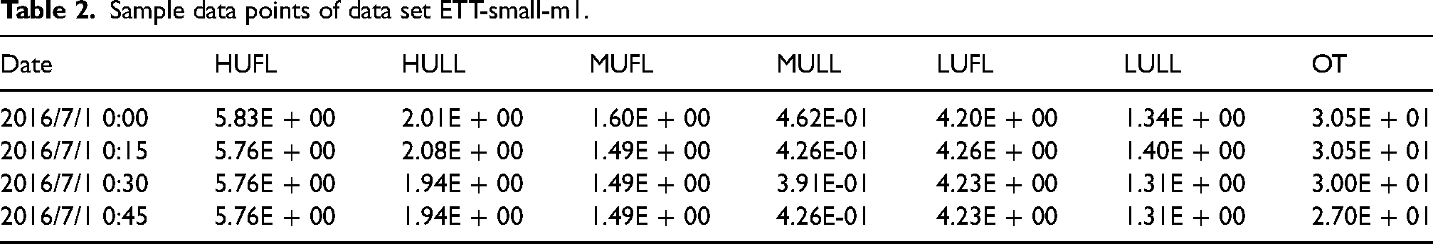
The data set adopts the ETT small data set in the power transformer data set, 22 which has been published at https://github.com/zhouhaoyi/ETDataset. The ETT-small data set contains data from two power transformers for 2 years. Each data point marked with m is recorded every minute from two regions in the same province of China, named ETT-small-m1 and ETT-small-m2. In addition, we use h to mark the dataset variants with 1 hour granularity, namely ETT-small-h1 and ETT-small-h2. Each data point has eight-dimensional characteristics, including the recording date of the data point, the predicted value “oil temperature,” and six different kinds of external load values, which are HUFL, HULL, MUFL, MULL, LUFL, and LULL. The missing values in the data have been pre-processed with the cleaning method. The data set is very important for the research of the time series. The data is real and effective, and the amount of data is also very large. The ETT-small-h1 and ETT-small-m1 data set was used in this experiment, whose sample data are shown in Tables 1 and 2.
Sample data points of data set ETT-small-h1.

Sample data points of data set ETT-small-m1.
Data prediction with EMD-BiLSTM model
Build BiLSTM model
The experimental environment is Pycharm. Python's keras library is called to build the BiLSTM network. The activation function is the tanh function by default. The mean square error (MSE) is used as the loss function. 80% of the data set is trained 100 times as a training set, and the rest is a test set for prediction. The iterative update algorithms used for BiLSTM include Adagrad algorithm, Adam algorithm, and RMSProp. According to prediction and fitting effect, RMSprop algorithm is used in this experiments.
Decomposition data using EMD
The time series of oil temperature in power tranformer can be regarded as nonlinear and nonstationary signals. Therefore, EMD is employed to extract mono-component and symmetric components from the nonlinear and nonstationary signals by a filtering process. The filtering process is to remove the lowest frequency information until only the highest frequency remains. The EMD results contain a series of IMFs and a residual. At ETT-small-h1 Ot variables are extracted from CSV data set. A total of 17,421 pieces of Ot variables are decomposed by EMD and the results are shown Figure 5.
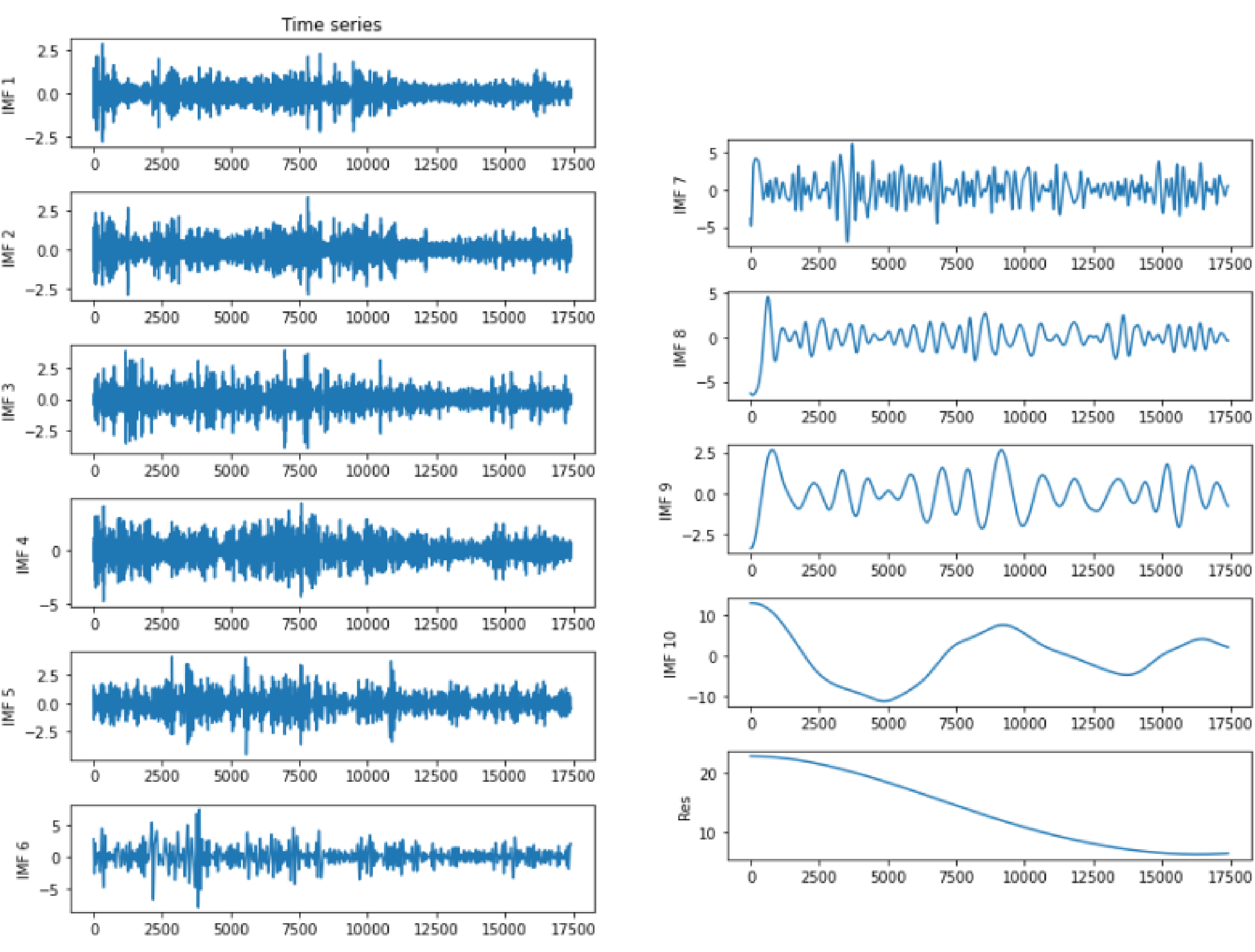
EMD components and residual.
From Figure 5, we can find that the time series finally are decomposed into 10 IMF components and 1 residual component. At the same time, it is demonstrated that all the 10 IMF components satisfy the following conditions: the number of extreme and the number of zero crossings is either equal or differ at most by one; at any point, the mean value of the envelope defined by the local maxima and the local minima is zero. For the residual component, it is a monotonic decreasing function which indicates no more IMF can be extracted.
Data prediction
The BiLSTM network is used to model and predict the component data respectively. Finally, the prediction results of every component are reconstructed. And then the RMSE, MAE, and MAPE were selected to evaluate the effectiveness of the proposed method. We assume that Oi and Pi are the observed (ground truth) and predicted values, respectively. These indicators can be formulated as follows.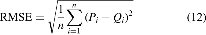


Prediction results comparison on data set ETT-small-h1.

Prediction results comparison on data set ETT-small-m1.
Prediction accuracy comparison results on data set ETT-small-h1.

Prediction accuracy comparison results on data set ETT-small-m1.

Conclusion
As a critical power transmission and transformation equipment, power transformers generate large volumes of time-series data on oil temperature during operation. Extracting useful information from this data can help to monitor the running state of power transformers in real-time, directly impacting the reliability of the power system and power supply. In this work, we propose a technique for forecasting transformer oil temperature based on EMD-BiLSTM. The method uses BiLSTM neural networks and EMD. The only inputs required for this model are time-series data on the temperature of the transformer oil, which is treated as signal data. EMD is used to break down the data and extract frequency and amplitude characteristics as an unsupervised feature learning technique. This approach improves the ability to anticipate short-term trends, particularly for abrupt shifts. In the supervised learning phase, BiLSTM is utilized. The monitored transformer data can be used to predict the transformer's functioning condition in the future, which has tremendous research value.
Footnotes
Declaration of conflicting interests
The author(s) declared no potential conflicts of interest with respect to the research, authorship, and/or publication of this article.
Funding
The author(s) received no financial support for the research, authorship, and/or publication of this article.