Research on parallel parking path planning and tracking control of unmanned vehicles

Abstract

Aiming at the problems of discontinuous curvature of the planned path, difficulty in finding the optimal reference path and high control accuracy requirements in tracking control for unmanned vehicles in the process of parallel parking, an optimal reference path planning method based on arc line and multi-objective optimization function and a path tracking control strategy based on nonlinear model predictive control are proposed. Firstly, the upper and lower boundaries of the exercisable area are obtained by the tangent of the arc and the straight line, and the multi-objective optimization function is designed to obtain the optimal arc-line combination, and the optimal reference path is obtained by polynomial curve fitting. Secondly, a path-following controller is designed using nonlinear model predictive control. Finally, a comparative analysis is carried out in MATLAB/Simulink and Carsim with the controller based on pure tracking design. The results show that the optimal reference path curvature obtained by the proposed method is continuous without sudden change, and the designed tracking controller has better tracking accuracy.

Introduction

With the rapid development of unmanned vehicles, the Automated Parking System (APS), plays an important role in reducing the burden on drivers and improving vehicle safety. ¹ APS consists of three steps: environmental perception, path planning, and path tracking. Among them, the last two steps play a key role in the success of parking and determine the efficiency, accuracy, and safety of automatic parking.

For path planning problem, the existing parking path planning method can be roughly divided into two types. ² The first kind of planning method is based on an optimization algorithm. Li et al. ³ established the parking path optimization problem by planning the optimal path time and using the interior point synchronous dynamic optimization method to solve the parking path. Chai et al. ⁴ use particle swarm optimization algorithm and adaptive gradient method to solve the parking path by aiming at the shortest parking path and minimum pose deviation. Although the above path planning method based on the optimization algorithm has no constraint on the initial parking position and pose of vehicles and has a wide range of applications, it is difficult to be generalized and applied due to its large amount of calculation and low efficiency. Another kind of planning method is based on a geometry curve. Sungwoo et al. ⁵ plan the shortest parking path by means of the tangent of two arcs, and there is the problem of spin turning because the curvatures at the tangent are not connected. Some scholars use the Bessel curve, cyclotron curve, B-spline curve, and so on to smooth the parking path so that the path curvature changes continuously.^6–9 Although the above geometric curve planning method has higher computational efficiency and is convenient for engineering implementation relative to the optimization planning method, there are still some shortcomings, such as the acceleration is difficult to change continuously and smoothly, the whole reference path is long, and it is difficult to find the optimal reference path.

While the quintic polynomial can ensure the smoothing jerk and can specify the velocity and acceleration of the starting and ending path points, overcome the shortcomings of the geometric curve planning method. ¹⁰

For the path tracking problem, the existing parking path tracking methods mainly include pure tracking control, synovial control, and fuzzy control methods. Li et al. ¹¹ use an improved pure tracking method to track polynomial curves. Jiang et al. ¹² use a non-time reference terminal for reaching law. The sliding mode path tracking control method is used to reduce the tracking error, improve the approach quality, and track the trajectory. Wen et al. ¹³ make the tracking of parking path by establishing a simplified fuzzy rule library and using a learning algorithm to optimize the parameters of the fuzzy controller. Xiong et al. ¹⁴ use the distance-angle deviation as a lateral preview model and used fuzzy control to design a fuzzy controller to track the parking path. Although the above methods have a good tracking effect on automatic parking, it is difficult to solve the problems of large changes in the curvature and heading angle of the reference path with low vehicle speed and the high requirements for tracking control accuracy in automatic parking. Nonlinear model predictive control (NMPC) can correct the control errors caused by model mismatch and external disturbances in time by through rolling optimization and feedback adjustment, it can better meet the requirements of automatic parking tracking control.

For the reasons mentioned above, this article proposes an optimal reference path planning method based on arc-line and multi-objective optimization functions, and a nonlinear model-based predictive path tracking control strategy. First, the upper and lower boundaries of the exercisable area are obtained by the tangent of the arc and the straight line, and the multi-objective optimization function is designed to obtain the optimal arc-line combination, and the optimal reference path is got by polynomial curve fitting. Then a path-following controller is designed using nonlinear model predictive control. Finally, the proposal is simulated in MATLAB/Simulink and Carsim compared with the pure tracking control.

Vehicle kinematics model

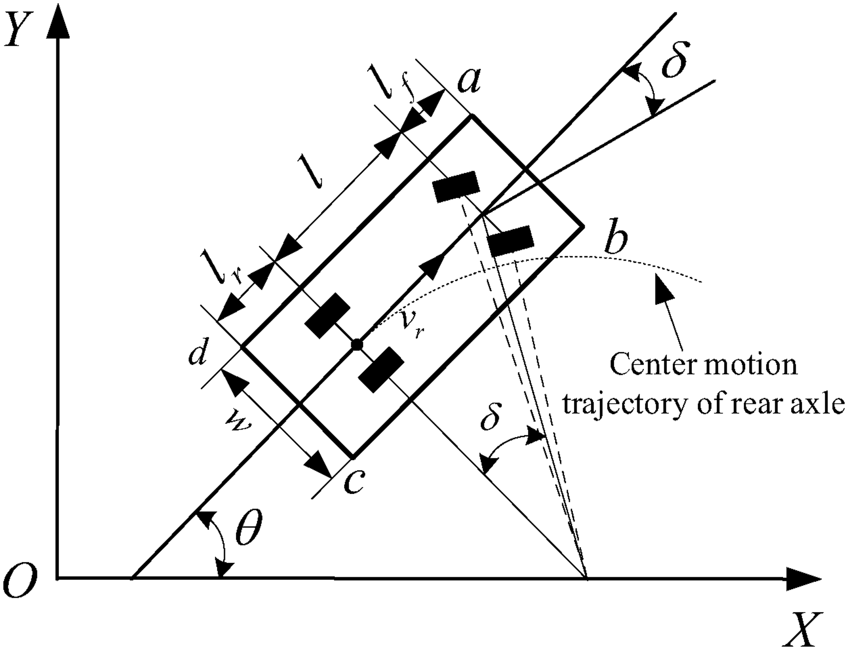
The unmanned vehicle is in a low-speed driving state during the parking process, and the influence of tire side slip can be ignored. The vehicle is simplified as a rigid body, and the path tracking controller is designed with the vehicle kinematic model instead of the dynamic model, and the center coordinate of the rear axle of the vehicle is used to design the path tracking controller. The motion state of the vehicle is represented by the center coordinates of the rear axle of the vehicle, and the kinematics model of the vehicle can be derived as follows:

$$\{\begin{array}{c}\dot{x}=v_r\cos \theta \\ \dot{y}=v_r\sin \theta \\ \dot{\theta }=(v_r\tan \delta )/l\end{array}$$

(1)

where $\dot{x}$ and $\dot{y}$ are the velocity components of the vehicle at X and Y, respectively, $v_r$ is the rear axle speed, l is the wheel base, $\delta$ is the front wheel angle, $\theta$ is the heading angle, and $\dot{\theta }$ is yaw velocity.

The established vehicle kinematics model is shown in Figure 1.

Figure 1.

Vehicle kinematics model, where a, b, c, and d represent the four vertices of the vehicle contour, $l_f$ is the front suspension of vehicle, $l_r$ is the rear suspension of vehicle, and w is the width of the car.

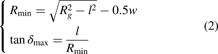
When the vehicle runs with the minimum turning radius, the following relationship exists between the minimum turning radius $R_g$ of the vehicle, the maximum front wheel angle ${\delta }_{max}$ and the minimum turning radius $R_{max}$ of the rear axle center:

$$\{\begin{array}{c}{R}_{min}=\sqrt{R_g^2-l^2}-0.5w\\ \tan {\delta }_{max}={\displaystyle \frac{l}{R_{min}}}\end{array}$$

(2)

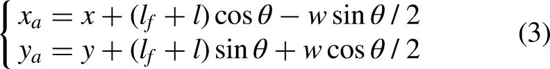
The coordinate relationship between the four vertices of the body and the center point of the rear axle is

$$\{\begin{array}{c}{x}_a=x+(l_f+l)\cos \theta -w\sin \theta /2\\ y_a=y+(l_f+l)\sin \theta +w\cos \theta /2\end{array}$$

(3)

$$\{\begin{array}{c}{x}_b=x+(l_f+l)\cos \theta +w\sin \theta /2\\ y_b=y+(l_f+l)\sin \theta -w\cos \theta /2\end{array}$$

(4)

$$\{\begin{array}{c}{x}_c=x-l_r\cos \theta +w\sin \theta /2\\ y_c=y-l_r\sin \theta -w\cos \theta /2\end{array}$$

(5)

$$\{\begin{array}{c}{x}_d=x-l_r\cos \theta -w\sin \theta /2\\ y_d=y-l_r\sin \theta +w\cos \theta /2\end{array}$$

(6)

Optimal reference path design

To realize the design of the optimal reference path, as shown in Figure 2. When the starting point and ending point coordinates of the parking are known, the arc radius of the first and second segments of the upper and lower boundaries of the exercisable area and the coordinates of the intersection between the arc and the straight line are solved by using the arc line tangent method, according to the starting point, ending point, collision avoidance constraints and vehicle parameter constraints. So as to determine the exercisable area of the parking trajectory. Three evaluation indexes of path curvature, control of the adjustable margin, and path length are designed to obtain the optimal arc-line combination in the exercisable area, and the optimal reference path is obtained by smoothing them with polynomial curves.

Figure 2.

Optimal reference path analysis, where $m_1$ and $m_4$ are the starting point and ending point coordinates of the vehicle, $m_{22}$ , $m_{32}$ , $m_{21}$ , and $m_{31}$ are the coordinates of the upper and lower boundaries of the drivable region at the intersection points of straight lines, $R_{21max}$ , $R_{22min}$ , $R_{11min}$ , and $R_{12max}$ the radius of the upper and lower boundary of the driving area, $O_{21}$ , $O_{22}$ , $O_{11}$ , and $O_{12}$ are center coordinates of the upper and lower boundaries of the driving area.

Determination of the lower boundary of the drivable area

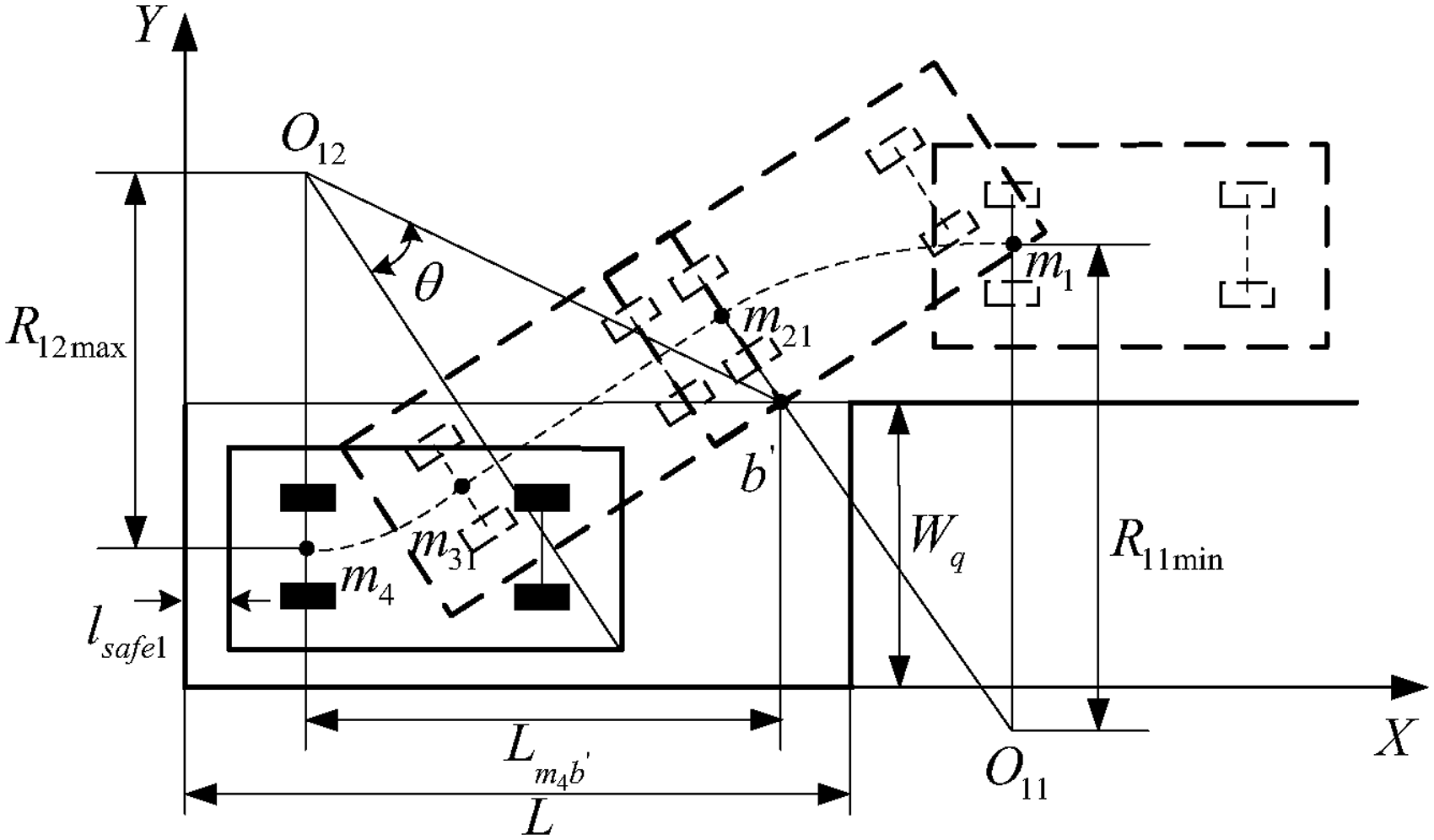
Under ideal conditions, the end of the parking should be located in the middle of the parking space as far as possible. Considering the parking safety, the end of the parking should be set as $m_4(l_{safe1}+l_r,0.5W_q)$ . As shown in Figure 3, safety distances $l_{safe1}$ and $l_{safe2}$ are reserved to ensure the safety of parking. By using reverse analysis (vehicle leaves from the parking space), according to the right front point b of the car body does not collide with the vertex $A^{\mathrm{\prime }}$ of the parking space, the radius $R_{12max}$ of the second section of the lower boundary of the drivable area can be obtained

$$\begin{array}{rl}& (R_{12max}+0.5w{)}^2+(l+l_f{)}^2\\ & =(R_{12max}-0.5W_q{)}^2+(L-l_r-l_{safe1}-l_{safe2}{)}^2\end{array}$$

(7)

Figure 3.

Analysis of radius $R_{12max}$ of the second section of the lower boundary of the drivable area. where A, B, C, and D represent the four vertices of parking space, L is the length and $W_q$ is the width of the parking space.

When b moves to point $A^{\mathrm{\prime }}$ , the vehicle heading angle $\theta$ can be calculated

$$\begin{array}{rl}& \theta =\arctan \left({\displaystyle \frac{L_{m_4{b}^{\mathrm{\prime }}}}{R_{12max}-0.5W_q}}\right)\\ & -\arctan \left({\displaystyle \frac{(l+l_f)}{(R_{12max}+0.5w)}}\right)\end{array}$$

(8)

where $L_{m_4{b}^{\mathrm{\prime }}}=\sqrt{R_b^2-{(R_{12max}-0.5W_q)}^2}$ is the vertical distance from $m_4$ to $b^{\mathrm{\prime }}$ , and the coordinates of the center point $m_{31}$ of the rear axis are as follows:

$$\begin{array}{rl}& (x_{m31},y_{m31})=(l_{safe2}+l_r+R_{12max}\sin \theta ,\\ & R_{12max}(1-\cos \theta )+0.5W_q)\end{array}$$

(9)

When the center point of the rear axle passes through point $m_{31}$ , it drives along the line $m_{31}{m}_{21}$ , so that the line equation of the lower boundary of the drivable area is $y=a_{1}x+b_1$ , and the heading angle of the vehicle at $m_{31}$ is also $\theta$ , the line equation can be obtained as

$$\{\begin{array}{c}{a}_1=\tan \theta \\ b_1=y_{m31}-a_1{x}_{{}_{m31}}\end{array}$$

(10)

Since the planned path arc is tangent to the straight line, the first arc of the lower boundary of the drivable area also passes through point $m_{21}$ .

From the formula of the distance from the center $O_{11}(x_{m1},y_{m1}-R_{11min1})$ to the line $y=a_{1}x+b_1$ , the first limit value $R_{11min1}$ of the first arc radius of the lower boundary of the drivable area can be obtained

$$R_{11min1}={\displaystyle \frac{|a_1{x}_{m1}+b_1-(y_{m1}-R_{11min1})|}{\sqrt{a_1^2+1}}}$$

(11)

The radius of the first section of the lower boundary of the drivable area calculated by the reverse analysis above cannot guarantee that the left front point a and right rear point c of the car body do not collide with the road boundary and parking space $A^{\mathrm{\prime }}$ . Therefore, by making the left front point a of the vehicle body not collide with the road boundary and reserving a safe distance $l_{safe3}$ , the second limit value $R_{11min2}$ of the first arc radius of the lower boundary of the drivable area is obtained, as shown in Figure 4.

$$\begin{array}{rl}& \sqrt{{(R_{11min2}+0.5w)}^2+{(l+l_f)}^2}\\ & =R_{11min2}-y_{m1}+H+W_q-l_{safe3}\end{array}$$

(12)

Figure 4.

Analysis of radius $R_{11min2}$ of the first section of the lower boundary of the drivable area.

Since the right rear point c of the car body does not collide with the parking space $A^{\mathrm{\prime }}$ , the third limit value q of the first arc radius of the lower boundary of the drivable area can be calculated, as shown in Figure 5.

$$\begin{array}{rl}(R_{11min3}-0.5w{)}^2=& (R_{11min3}-y_{m1}+W_q{)}^2\\ & +(x_{m1}-L+l_{safe2}{)}^2\end{array}$$

(13)

Figure 5.

Analysis of radius $R_{11min3}$ of the first section of the lower boundary of the drivable area.

When $R_{11min1}>max\{R_{11min2},R_{11min3}\}$ , $R_{11min}=R_{11min1}$ .

When $R_{11min1}<max\{R_{11min2},R_{11min3}\}$ , $R_{11min}=max\{R_{11min2},R_{11min3}\}$ , it is necessary to reversely deduce the radius $R_{12max}$ of the second arc of the lower boundary of the new drivable area and the straight line equation $y=a_{1}x+b_1$ of the lower boundary of the drivable area, as shown in Figure 6.

Figure 6.

Analysis of radius $R_{12max}$ of the second section of the lower boundary of the drivable area.

The distance from the center of the circle $O_{11}(x_{m1},y_{m1}-R_{11min})$ to the straight line $y=a_{1}x+b_1$ is $R_{11min}$ .

$$R_{11min}={\displaystyle \frac{|a_1{x}_{m1}+b_1-(y_{m1}-R_{11min})|}{\sqrt{a_1^2+1}}}$$

(14)

The distance from the center of the circle $O_{12}(l_r+l_{safe1},R_{12max}+0.5W_q)$ to the straight line $y=a_{1}x+b_1$ is $R_{12max}$ .

$$R_{12max}={\displaystyle \frac{|a_1(l_r+l_{safe1})+b_1-(R_{12max}+0.5W_q)|}{\sqrt{a_1^2+1}}}$$

(15)

When the right front point b of the car body moves to intersect the upper-end line of the parking space, there is no collision occurs between the car body points and the parking space when the vehicle is traveling in a straight line. The heading angle $\theta$ of the new vehicle can be obtained by the same formula (8). In this case, the slope of the linear equation of the lower boundary of the drivable area is equal to the tangent value of $\theta$ .

$$a_1=\tan \theta$$

(16)

Combined with (14) to (16), $y=a_{1}x+b_1$ and $R_{12max}$ are obtained.

Determination of upper boundary of drivable area

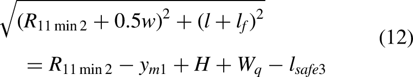
To ensure that the right rear point c of the car body does not collide with the lower edge of the parking space, the first limit value $R_{22min1}$ of the second arc radius of the upper boundary of the drivable area is determined, as shown in Figure 7.

$$(R_{22min1}+0.5w{)}^2+l_r^2=(R_{22min1}+0.5W_q{)}^2$$

(17)

Figure 7.

Analysis of radius $R_{22min1}$ of the second arc on the upper boundary of the drivable area.

Meanwhile, to meet the constraints of the vehicle steering mechanism, the radius $R_{22min}$ of the second arc on the upper boundary of the drivable area should meet the following requirements

$$R_{22min}=max(R_{22min1},R_{min})$$

(18)

In the same way, the equation $y=a_{2}x+b_2$ of the straight line and the radius $R_{21max}$ of the first arc in the upper boundary of the drivable area are obtained from formulas (8) to (10).

Design of multi-objective optimization function

After the upper and lower boundary of the drivable area is calculated based on the arc straight line, theoretically, any group of arc-line combinations in the drivable area can meet the requirements of parking path planning. In this article, considering the influence of path curvature change, control adjustable margin, and path length on the reference path, a multi-objective optimization function is designed to find the optimal combination of circular arc lines in the drivable area.

Smooth curvature change

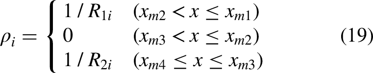
To avoid large turning angles in the parking process, the path curvature should be as small as possible. The two arcs in the driving area are discretized. The radius of the first arc is $R_{1i}$ , the radius of the second arc is $R_{2i}$ , and the curvature of the reference path ${\rho }_i$ is

$${\rho }_i=\{\begin{array}{cc}1/R_{1i}& (x_{m2}<x\le x_{m1})\\ 0& (x_{m3}<x\le x_{m2})\\ 1/R_{2i}& (x_{m4}\le x\le x_{m3})\end{array}$$

(19)

where $x_{m1}$ and $x_{m2}$ are the abscissa of the intersection point of the first arc, the second arc, and the line, respectively. According to the values of $R_{1i}$ and $R_{2i}$ , the equation $y=ax+b$ of the line is obtained from the distance formula of the coordinates $O_1(x_{m1},y_{m1}-R_{1i})$ and $O_2(l_{safe1}+l_r,0.5W_q+R_{2i})$ of the center of the two arcs to the line.

$$\{\begin{array}{c}{R}_{1i}={\displaystyle \frac{|a{x}_{m1}+b-(y_{m1}-R_{1i})|}{\sqrt{a^2+1}}}\\ R_{2i}={\displaystyle \frac{|a(l_{safe2}+l_r)+b-(R_{2i}+0.5W_q)|}{\sqrt{a^2+1}}}\end{array}$$

(20)

The coordinate $m_2(x_{m2},y_{m2})$ of the intersection of the first arc and the line is obtained from the intersection of the arc and the line

$$\{\begin{array}{c}{R}_{1i}^2={(x_{m2}-x_{m1})}^2+{(y_{m2}-(y_{m1}-R_{1i}))}^2\\ y_{m2}=a{x}_{m2}+b\end{array}$$

(21)

Similarly, the coordinate $m_3(x_{m3},y_{m3})$ of the intersection of the second arc and the line is obtained.

When the radius of the first arc and the radius of the second arc are maximized, the path curvature is minimized and when both radiuses of the arc are minimized, the path curvature is maximized.

$$\{\begin{array}{c}{\rho }_{min}=1/R_{12max}+1/R_{21max}\\ {\rho }_{max}=1/R_{11min}+1/R_{22min}\end{array}$$

(22)

The path curvature ${\rho }_i$ is constrained as

$${\rho }_{min}\le {\rho }_i\le {\rho }_{max}$$

(23)

Maximum control adjustable margin

Control adjustable margin indicates the size of the correction controllable domain in vehicle control if the vehicle deviates from the expected trajectory. Since the variation range of the vehicle's steering angle is smaller than that of the vehicle's turning radius, the radius margin of the reference path is transformed into the front wheel angle margin ${\beta }_i$

$${\beta }_i=\{\begin{array}{cc}\arctan (l/R_{1i})& (x_{m2}<x\le x_{m1})\\ 0& (x_{m3}<x\le x_{m2})\\ \arctan (l/R_{2i})& (x_{m4}\le x\le x_{m3})\end{array}$$

(24)

When the radius of the first arc and the radius of the second arc are maximized, the front wheel angle margin is minimized and when both radiuses of the arc are minimized, the front wheel angle margin is maximized.

$$\{\begin{array}{c}{\beta }_{min}=\arctan (l/R_{21max})+\arctan (l/R_{12max})\\ {\beta }_{max}=\arctan (l/R_{11min})+\arctan (l/R_{22min})\end{array}$$

(25)

The front wheel angle margin ${\beta }_i$ is constrained as

$${\beta }_{min}\le {\beta }_i\le {\beta }_{max}$$

(26)

Shortest path length

When the parking speed is constant, the shorter the planned parking path length is, the shorter the parking time will be. The path length indicates the time required for the whole parking process, and the path length can reflect the economic performance of parking without considering other factors. The length of the parking path curve can be represented by the total arc length $s_i$ of the parking path curve

$$s_i=\{\begin{array}{cc}{\phi }_1{R}_{i1}& (x_{m2}<x\le x_{m1})\\ {\int }_{x_{m3}}^{x_{m2}}\sqrt{1+{y^{\mathrm{\prime }}}^2}dx& (x_{m3}<x\le x_{m2})\\ {\phi }_2{R}_{2i}& (x_{m4}\le x\le x_{m3})\end{array}$$

(27)

where ${\phi }_1$ is the rotation angle of the rear axle center moving from point $m_1$ to point $m_2$ , ${\phi }_2$ is the rotation angle of the rear axle center moving from point $m_3$ to point $m_4$ .

When the radius of the first arc and the radius of the second arc are maximized, the length of the path is maximized and when both radiuses of the arc are minimized, the length of the path is minimized.

$$\{\begin{array}{c}{s}_{min}={\phi }_1{R}_{11min}+{\int }_{x_{m3}}^{x_{m2}}\sqrt{1+{y^{\mathrm{\prime }}}^2}dx+{\phi }_2{R}_{22min}\\ s_{max}={\phi }_1{R}_{21max}+{\int }_{x_{m3}}^{x_{m2}}\sqrt{1+{y^{\mathrm{\prime }}}^2}dx+{\phi }_2{R}_{12max}\end{array}$$

(28)

The length of the path $s_i$ is constrained as

$$s_{min}\le s_i\le s_{max}$$

(29)

Multi-objective optimization function

According to the above analysis, when the path length is the shortest, the curvature of the path is not soft, and the adjustable margin at any time is not the maximum, which is contradictory to each other. Therefore, the following evaluation function is designed to calculate its substitute value.

$$\begin{array}{c}min{F}_i=k_1{\overline{\rho }}_i+k_2{\overline{\alpha }}_i+k_3{\overline{s}}_i\\ s.t.\{\begin{array}{c}{\rho }_{min}\le {\rho }_i\le {\rho }_{max}\\ {\beta }_{min}\le {\beta }_i\le {\beta }_{max}\\ \begin{array}{c}{s}_{min}\le s_i\le s_{max}\\ {\alpha }_i=1/{\beta }_i\end{array}\\ k_1+k_2+k_3=1\\ 0<k_1<1\\ 0<k_2<1\\ 0<k_3<1\end{array}\end{array}$$

(30)

where $k_1$ , $k_2$ , and $k_3$ are the weight coefficients, ${\rho }_i$ is the path curvature, ${\beta }_i$ is the front wheel angle margin, $s_i$ is the path length, ${\overline{\rho }}_i=\frac{{\rho }_i-{\rho }_{min}}{{\rho }_{max}-{\rho }_{min}}$ , ${\overline{\alpha }}_i=\frac{{\alpha }_i-{\alpha }_{min}}{{\alpha }_{max}-{\alpha }_{min}}$ , and ${\overline{s}}_i=\frac{s_i-s_{min}}{s_{max}-s_{min}}$ .

In summary, the radius of the first arc $R_1$ and the radius of the second arc $R_2$ are calculated from equation (30) when the evaluation function is minimized. According to equations (20) and (21), the linear equation $y=ax+b$ and the coordinates $m_2(x_{m2},y_{m2})$ and $m_3(x_{m3},y_{m3})$ of the intersection point between the two arcs and the line can be obtained, so that the optimal combination of arc lines in the driving area can be obtained.

Optimal reference path smoothing

The parking reference path should meet the requirements of no collision with surrounding obstacles, continuous path curve, zero slope of the starting point and ending point, continuous curvature, and no more than the minimum turning radius of the vehicle. ¹⁵ Curvature discontinuity exists in the reference path obtained by the tangent of the circular arc line. To tackle this issue, different types of curves are proposed. The advantages and disadvantages of common path curves are shown in Table 1. It can be seen that the quintic polynomial can meet the requirement of continuous curvature and is easy to solve. Therefore, this article chooses the quintic polynomial to fit the optimal circular arc line.

Table 1.

Comparison of advantages and disadvantages of different path curves.

Path curves type	Advantage	Disadvantages
B-spline curve Bezier curve	Continuous curvature. Easy to track	Much parameters. Higher calculation burden
Arctangent function Sigmoid function	Lower calculation burden. Continuous and smooth curvature	Not zero curvature at starting/ending points
Sinusoidal and polynomial superimposed curves	Continuous and smooth curvature.	Much parameters. Sometimes no solution
Quintic polynomial curve	Lower calculation burden. Continuous and smooth curvature	Larger parking space required

The planned parking path needs to pass through the starting coordinate $m_1(x_{m1},y_{m1})$ and the ending coordinate $m_4(x_{m4},y_{m4})$ of the parking, and the following constraint equation can be established

$$y_{m1}=k_4{x}_{m1}^5+k_5{x}_{m1}^4+k_6{x}_{m1}^3+k_7{x}_{m1}^2+k_8{x}_{m1}+k_9$$

(31)

$$y_{m4}=k_4{x}_{m4}^5+k_5{x}_{m4}^4+k_6{x}_{m4}^3+k_7{x}_{m4}^2+k_8{x}_{m4}+k_9$$

(32)

where $k_4\sim k_9$ are the coefficients of the quintic polynomial; $x_{m1}\sim x_{m4}$ and $y_{m1}\sim y_{m4}$ are the coordinates of $m_1\sim m_4$ .

To fit the arc line, the fifth-degree polynomial curve needs to pass through the coordinate $m_2(x_{m2},y_{m2})$ of the intersection point between the first arc and the line and the coordinate $m_3(x_{m3},y_{m3})$ of the intersection point between the second arc and the line. The following constraint equation can be established

$$y_{m2}=k_4{x}_{m2}^5+k_5{x}_{m2}^4+k_6{x}_{m2}^3+k_7{x}_{m2}^2+k_8{x}_{m2}+k_9$$

(33)

$$\begin{array}{r}{y}_{m3}=k_4{x}_{m3}^5+k_5{x}_{m3}^4+k_6{x}_{m3}^3+k_7{x}_{m3}^2+k_8{x}_{m3}+k_9\end{array}$$

(34)

To satisfy that the position and pose of the vehicle in the starting and ending parking states are parallel to the parking space, the derivative of the quintic polynomial curve at the starting coordinate $m_1(x_{m1},y_{m1})$ and the ending coordinate $m_4(x_{m4},y_{m4})$ is zero, and the following constraint equation can be established

$$0=5k_4{x}_{m1}^4+4k_5{x}_{m1}^3+3k_6{x}_{m1}^3+2k_7{x}_{m1}+k_8$$

(35)

$$0=5k_4{x}_{m4}^4+4k_5{x}_{m4}^3+3k_6{x}_{m4}^3+2k_7{x}_{m4}+k_8$$

(36)

The simultaneous equations (31) to (36) can be used to find the coefficients of the quintic polynomial, which can be used as the final optimal reference path for parking.

Design of path tracking controller

Compared with the linear model prediction method, the NMPC does not require a linearization process for nonlinear systems, which makes the simplified mathematical model closer to the real system state. Its core is to establish the prediction model and rolling optimization function, which minimizes the tracking error on the premise of minimum control quantity. According to the vehicle kinematics model in formula (1), the vehicle system can be regarded as a control system whose input is the control quantity $u(\delta )$ and state quantity $\chi (x,y,\theta )$ , and its general form is

$$\dot{\chi }=f(\chi ,u)$$

(37)

where $\dot{\chi }$ is the derivative of $\chi$ ; x and y are the center coordinates of the rear axle of the vehicle; $\theta$ is the heading angle of the vehicle; $\delta$ is the front wheel angle of the vehicle.

In order to make the kinematics model applied to the design of a nonlinear model predictive controller, the Euler method is adopted to discretize formula (37).

$$\chi (t+1|t)=\chi (t|t)+Tf(\chi (t|t),u(t|t))$$

(38)

where t is the current sampling time; $t+1$ is the next sampling moment, and T is the sampling period and set to 0.05 s.

Assuming that the control time domain is $N_c$ and the prediction time domain is $N_p$ , the action sequence of the control quantity is

$$[u(t|t),u(t+1|t)\cdot \cdot \cdot u(t+N_c-1|t)]$$

(39)

where $u(t+1|t)$ is the control quantity at time $t+1$ .

In the prediction time domain, the pose state of the vehicle at each moment is

$$\begin{array}{rl}& \chi (t+1|t)=\chi (t|t)+Tf(\chi (t|t),u(t|t))\\ & ⋮\\ & \chi (t+N_c|t)=\chi (t+N_c-1|t)+Tf(\chi (t+N_c-1|t),u(t+N_c-1|t))\\ & \chi (t+N_c+1|t)=\chi (t+N_c|t)+Tf(\chi (t+N_c|t),u(t+N_c|t))\\ & ⋮\\ & \chi (t+N_p|t)=\chi (t+N_p-1|t)+Tf(\chi (t+N_p-1|t),u(t+N_p|t))\end{array}$$

(40)

The deviation between vehicle pose and reference path in the time domain, namely, the predicted error is

$$\begin{array}{c}e(t+i|t)=\chi (t+i|t)-{\chi }_{ref}(t+i|t)\\ i=1,2,3,\dots ,N{}_p\end{array}$$

(41)

where ${\chi }_{ref}$ is the position and pose state information of the tracking target point on the reference path.

Based on the above model, the objective function of rolling optimization can be designed as

$$\begin{array}{c}J(e(t),u(t))=\sum _{i=1}^{N_p}{\Vert e(t+i|t)\Vert }_{Q_1}^2\\ +\sum _{i=1}^{N_c-1}{\Vert \mathrm{\Delta }u(t+i|t)\Vert }_{Q_2}^2+\sum _{i=1}^{N_c-1}{\Vert \delta (t+i|t)\Vert }_{Q_3}^2+\Vert \epsilon {\Vert }_{Q_4}^2\end{array}$$

(42)

where the first item on the right of the equation is the tracking error penalty item, indicating the ability of the controlled system to follow the reference trajectory. The second term is the penalty of control input increment, reflecting the requirement of steady change of control quantity. The third term is the control quantity penalty to prevent the frequent changes in front wheel rotation caused by a small disturbance in the parking process. The last term prevents the occurrence of no feasible solution during operation. $Q_1$ , $Q_2$ , $Q_3$ , and $Q_4$ are the weight coefficient matrixes. $\xi$ is the relaxation factor.

Control quantity constraint and control quantity increment constraint of the system should be considered in rolling optimization

$$\{\begin{array}{c}{u}_{min}(t+i|t)\le u(t+i|t)\le u_{max}(t+i|t)\\ i=0,1,2,\dots ,N_c-1\\ \mathrm{\Delta }{u}_{min}(t+i|t)\le \mathrm{\Delta }u(t+i|t)\le \mathrm{\Delta }{u}_{max}(t+i|t)\\ i=0,1,2,\dots ,N_c-1\end{array}$$

(43)

In parking path tracking control, the constraints of steering angle and steering angle increment are mainly considered.

According to formula (2) and vehicle parameters, the range of steering angle is $-0.5585\mathrm{rad}\le \delta \le 0.5585\mathrm{rad}$ .

The steering angle increment $\mathrm{\Delta }\delta$ is calculated by the following formula

$$\mathrm{\Delta }\delta =T\dot{\delta }$$

(44)

where $\dot{\delta }$ is the steering angular velocity.

According to formula (44), the range of change in steering angle is $-0.0279\mathrm{rad}\le \mathrm{\Delta }\delta \le 0.0279\mathrm{rad}$ .

In summary, the nonlinear model predictive control takes the front wheel angle $u(\delta )$ as the control quantity, and the vehicle attitude $\chi (x,y,\theta )$ as the state quantity. Under the control quantity and control increment constraints, the automatic parking path tracking control problem is transformed into a quadratic programming problem for solving

$$\begin{array}{rl}& l\underset{u(t),\epsilon }{min}J(e(t),u(t))=\sum _{i=1}^{N_p}{\Vert e(t+i|t)\Vert }_{Q_1}^2\\ & +\sum _{i=1}^{N_c-1}{\Vert \mathrm{\Delta }u(t+i|t)\Vert }_{Q_2}^2+\sum _{i=1}^{N_c-1}{\Vert \delta (t+i|t)\Vert }_{Q_3}^2\\ & +\Vert \epsilon {\Vert }_{Q_4}^2-0.5585\mathrm{rad}\le \delta \le 0.5585\mathrm{rad}\\ & -0.0279\mathrm{rad}\le \mathrm{\Delta }\delta \le 0.0279\mathrm{rad}\end{array}$$

(45)

In each control cycle, the optimal sequence is obtained by solving formula (45), and the first element in the control sequence is applied to the controlled vehicle. The same process is repeated in the subsequent cycle such that the vehicle is controlled to track the best-planned trajectory.

To ensure the safety and comfort of vehicles in the parking process, parking speed is generally controlled below 5 km/h. ¹⁶ Proportional–integral–derivative speed tracking controller is used to set the parking speed control, and the expected speed is set as 3.6 km/h.

Simulation and analysis

To verify the feasibility of parallel parking path planning and tracking control of driverless vehicles, MATLAB/Simulink and CarSim are used for joint simulation. Taking the actual parameters of a car as an example. According to the relevant construction standard requirements of the industry standard “Garage Building Design Code” of the People's Republic of China, the actual car and parking space parameters are set in Carsim.¹⁷ The vehicle parameters and environmental parameters are shown in Table 2.

Table 2.

Vehicle parameters and environmental parameters.

Parameter	Symbol	Unit	Numerical value
Vehicle width	$w$	$\mathrm{m}$	1.774
The wheelbase	$l$	$\mathrm{m}$	2.640
Front suspension	$l_f$	$\mathrm{m}$	0.787
Rear suspension	$l_r$	$\mathrm{m}$	1.158
Minimum turning radius	$R_g$	$\mathrm{m}$	5.76
Parking space length	$L$	$\mathrm{m}$	6.8
Parking space width	$W_q$	$\mathrm{m}$	2.1
Road width	$H$	$\mathrm{m}$	3.5
Maximum front wheel steering angular speed	${\dot{\delta }}_{max}$	$\mathrm{rad}/\mathrm{s}$	0.5585

Path planning simulation

The starting coordinates of parking are set as (9.1580, 3.3870), and the safe distance is 0.1000 m. ¹⁸ $R_{min}$ = 4.2000 m is calculated by formula (2). By setting the combination of weights and coefficients of different values, the multi-objective evaluation function is used to find the minimum objective function value under each combination of weights and coefficients. The corresponding weight coefficient combination of the minimum value of all the minimum objective function values is obtained. As shown in Figure 8, only part of the weight coefficient combination and the corresponding objective function value are shown. The minimum value of the objective function is 0.7707, and the corresponding weight coefficient combination is $k_1$ = 0.3, $k_2$ = 0.5, and $k_3$ = 0.2, which is set as the weight coefficient of this article. The optimal combination of arcs and lines in the driving area is calculated in MATLAB as shown in Figure 9. The radiuses of the first and second arcs of the upper boundary are 8.8918 m and 4.2000 m, respectively. The radiuses of the first and second arcs of the lower boundary are 8.1485 m and 4.7946 m, respectively. The radiuses of the first and second sections of the optimal arc-line combination are 8.4385 m and 4.3928 m, respectively, and the optimal arc-linear combination is located near the center of the drivable area. Figure 10 shows the simulation results of path curve fitting commonly used in Table 1. It can be seen from the figure that the path fitted by the arctangent function and sigmoid function is difficult to meet the requirement that the starting point of parking is parallel to the parking space, and the fitting effect is poor. The B-spline curve has the best path-fitting effect, but it is difficult to find control points and complicated to solve. The polynomial curve can satisfy the requirement that the parking starting point is parallel to the parking space, and the fitting effect is better than the arctangent function and sigmoid function. Figures 11 and 12 show the comparison before and after fitting the arc line combination by the quintic polynomial. It can be seen that the curvature of the arc-line combination has curvature mutation points in the whole parking process. After fitting the quintic polynomial, the shape of the arc-line combination can be maintained, and the curvature of the path is a smooth curve with no curvature mutation phenomenon, which meets the requirements of parking path planning. Figure 13 shows the trajectory of the center of the rear axle of the vehicle. It can be seen that the optimal arc-line combination can effectively avoid the restrictions of the road boundary and the parking space boundary in the parking environment, and form a collision-free reference path.

Figure 8.

Value of weight coefficient.

Figure 9.

The optimal combination of arcs and straight lines in the drivable area.

Figure 10.

Different curve fitting comparison.

Figure 11.

Path after polynomial fitting.

Figure 12.

Path curvature after polynomial fitting.

Figure 13.

Movement track of the center of the rear axle of the vehicle.

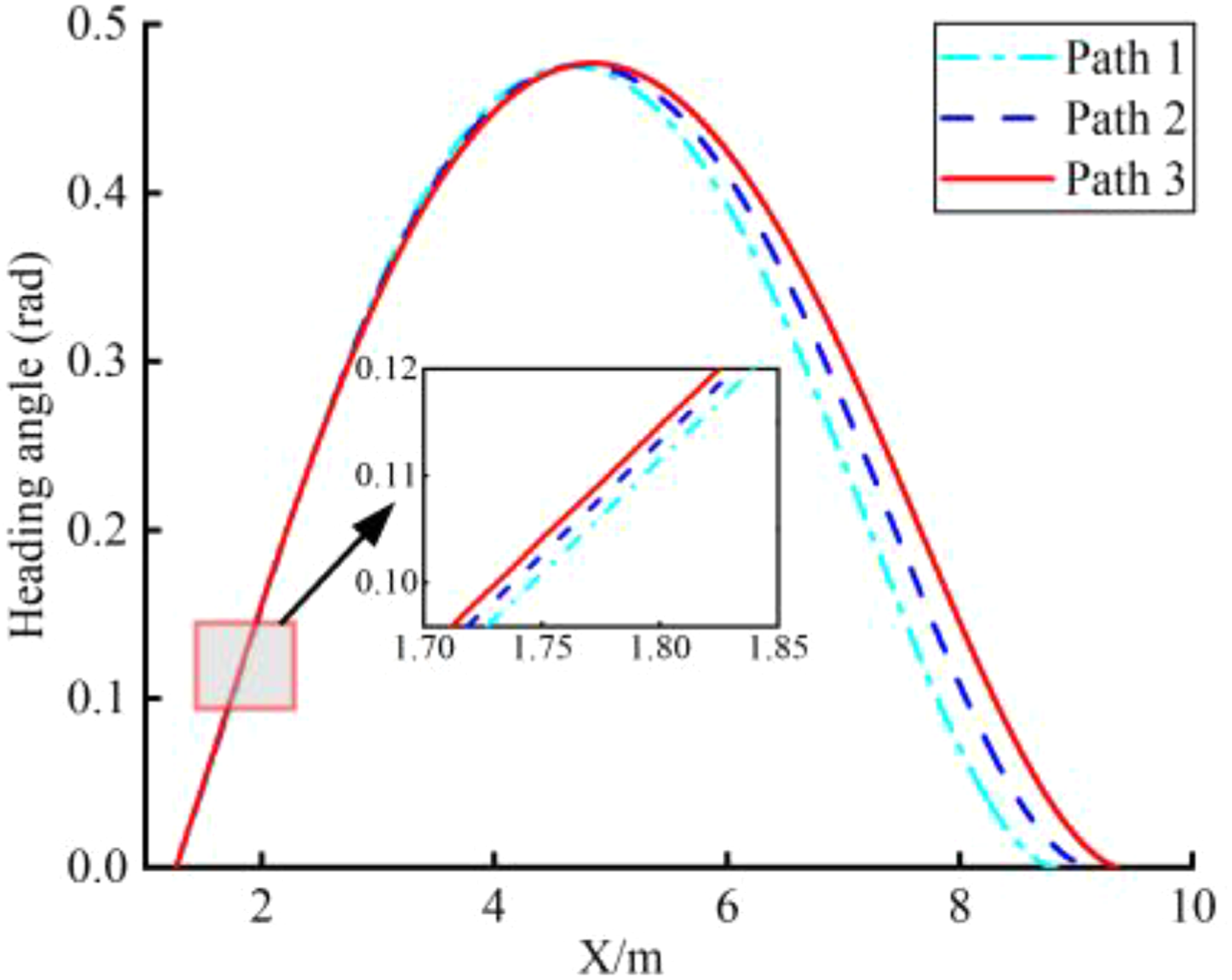
To verify the path planning performance of different parking starting points, the other two sets of starting point coordinates (9.3580, 3.4870) and (8.9580, 3.2870) are selected with the starting point (9.1580, 3.3870) in equal proportion, and the optimal reference path is obtained by quintic polynomial fitting. As shown in Figure 14, the heading angles of the vehicle at the starting point and the ending point are both 0, which meets the requirement that the initial state and the end state of the vehicle are parallel to the parking space. The three path curvatures are continuous without sudden change, the parking starting point curvature is 0, and the maximum curvature is 0.2124 m⁻¹, as shown in Figure 15, which meets the requirement of the maximum vehicle curvature of 0.2380 m⁻¹. The maximum front wheel rotation speed of the vehicle is 0.5325 rad/s, as shown in Figure 16, which meets the requirement of 0.5585 rad/s. Figure 17 shows the variation diagram of the front wheel angle of vehicles. It can be seen from the figure that the front wheel angle of vehicles continuously changes during the whole parking process. The maximum front wheel angle of vehicles in the three groups of paths is 0.5118 rad, which meets the requirement that the maximum front wheel angle of vehicles is less than 0.5585 rad. Taking the front wheel angle and path curvature as the evaluation index of ride comfort, the planned parking path meets the requirements of ride comfort.

Figure 14.

Vehicle heading angle.

Figure 15.

Path curvature.

Figure 16.

Vehicle front wheel angle speed.

Figure 17.

Front-wheel angle of vehicle.

Path tracking control simulation

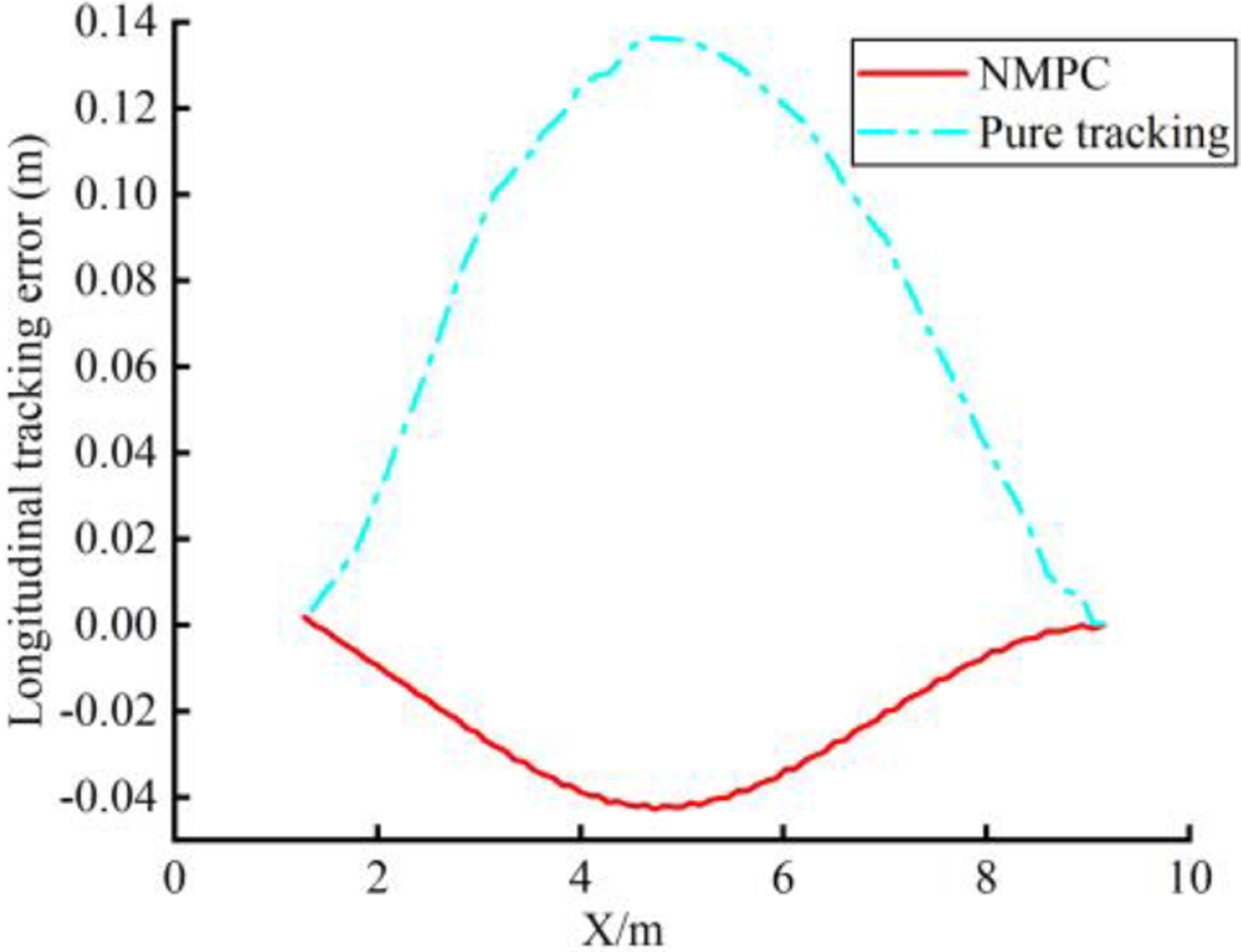
To verify the performance of the designed path tracking controller, the expected vehicle speed is set to −3.6 km/h. The coordinates of the starting point of the tracking reference path are set to (9.1580, 3.3870), and compared with the pure tracking algorithm. $Q_1$ , $Q_2$ , and $Q_3$ are empirical values determined by trial and error, It is found that when the ratio of heading error weight to transverse and longitudinal error weight in $Q_1$ is greater than 10 or the ratio of $Q_3$ to $Q_2$ is less than 1, the tracking error of the controller is larger, but the front wheel steering angle changes continuously without abrupt change. When the ratio of course error weight to transverse and longitudinal error weight in $Q_1$ is less than 10 or the ratio of $Q_3$ to $Q_2$ is more than 1, the tracking error of the controller is small, but the front wheel steering angle jumps. $\xi$ and $Q_4$ are relaxation factors and corresponding weight coefficients to prevent no solution phenomenon in the process of solving, set as $\xi$ = 5, $Q_4$ = 10. The controller parameters are shown in Table 3. It can be seen from Figures 18 and 19 that the vehicle can track the reference trajectory well under both NMPC and pure tracking control. However, it can be clearly seen from the local enlarged picture that the effect of NMPC tracking the reference trajectory is significantly higher than that of pure tracking control. The designed NMPC tracking controller can better meet the requirements of parking tracking control. It can be seen from Figure 20 that the tracking errors of the two tracking controllers are 0 at the starting point and the ending point, and the maximum error of pure tracking during the whole tracking process is 0.1365 m, accounting for 6.5% of the width of the parking space. The maximum ordinate tracking error of NMPC is 0.0428 m, accounting for 2.04% of the width of the parking space, whose tracking effect is significantly higher than pure tracking. Figure 21 shows that the maximum error of pure tracking heading angle reaches 0.0562 rad, while the maximum error of NMPC heading angle is 0.0165 rad, and the curve changes are more gentle than that of pure tracking control. Therefore, the tracking controller designed with NMPC has a better tracking effect than the controller with a pure tracking design.

Table 3.

Controller parameters.

The controller	Parameter selection
NMPC	$\begin{array}{rl}& Q_1=\left[\begin{array}{ccc}21& 0& 0\\ 0& 21& 0\\ 0& 0& 210\end{array}\right]Q_2=2\\ & Q_3=2Q_4=50\end{array}$
PID	$K_p=4K_i=0.5K_d=0.05$

NMPC: nonlinear model predictive control; PID: proportional–integral–derivative.

Figure 18.

Trajectory tracking effect.

Figure 19.

Heading angle tracking effect.

Figure 20.

Ordinate tracking error.

Figure 21.

Heading angle tracking error.

Conclusion

This paper proposes an optimal reference path planning method based on arc-line and multi-objective evaluation, and a nonlinear model-based predictive path tracking control strategy. The upper and lower boundaries of the exercisable area are obtained by the tangent of the arc and the straight line. The optimal arc-line combination is obtained by designing a multi-objective optimization function, and the optimal reference path is obtained by fitting the polynomial curve. Then a path-following controller is designed using nonlinear model predictive control. The simulation results show that the proposed method can not only satisfy the collision avoidance and vehicle parameter constraints, but also that the path curvature is continuous without mutation, and the tracking controller designed has better tracking accuracy.

This article studies and analyzes the parallel parking of unmanned vehicles, and this method can be improved and verified in vertical and inclined parking scenarios in the future. Although the curvature of the planned path is continuous and has no sudden change, it has high requirements on the attitude of the parking starting point and requires a large parking space size. A multi-step parking method will be considered in future work to reduce the impact of the attitude of the parking starting point and the size of the parking space.