
Abstract
This paper presents a verification study of wave propagation in fluid-filled elastic tubes using a coupled numerical simulation method by comparing the simulation results with analytical solutions. A three-dimensional fluid-structure interaction numerical model is built using Ansys software. Wave propagation is investigated by applying a pressure pulse at the inlet of a fluid-filled elastic tube. The speed of the pressure wave and the radial displacement of the tube are simulated and compared with theoretical values. Simulation results yield a high level of accuracy. Different structural elements are used to represent the tube, and their impact on the results is discussed. The effects of tube material, tube constraints and fluid properties are also investigated in this study.
Introduction
The pulse wave velocity (PWV), the pressure wave propagation speed, in a fluid-filled elastic tube is an important variable in the motion of such tubes. Experimentally the PWV can be determined by using pressure sensors placed at a known distance along a vessel. In blood flow, PWV is considered clinically as a measure of the performance of the arteries’ stiffness, which explains the large amount of work performed in this area. Besides being an excellent test case for FSI simulation, this problem is of direct interest. Our applications include modelling of an apparatus being developed to study digestion 1 and ducts containing replacement heart valves. 2
The equations relating to PWV have been developed for over a century. The most famous formula is the Moens-Korteweg equation,3,4 developed in 1878. They found that PWV depends on not only the elastic modulus of the structure, but also the geometrical dimensions of the tube and the fluid density. This equation is derived based on many assumptions and only accounts for the most important factors. A critical review of the equation is given by Lambossy. 5 Studies were carried out later by other researchers to provide more precise information on wave propagation characteristics.6–11 Most studies focused on estimating the elastic properties of the arterial wall and calculating the velocity of the blood flow through the measured PWV. Bergel12–14 modified the Moens-Korteweg equation by including two more parameters in the calculation, which are the Poisson's ratio and the ratio of thickness to outer radius of the tube. This modification compensates for the errors introduced by the use of the thin wall assumption of the Moens-Korteweg equation.
In the calculation of PWV, the arteries are assumed to be constrained axially, meaning that tube elongation is not considered. Therefore, the effect of tube constraints is not considered when estimating PWV in the circulatory system. However, it has been shown that the wave propagation velocity is also related to the longitudinal support of the tube.15–19 Different tube constraints can cause different fluid behaviours in an elastic tube. This finding is very important, particularly for the water hammer phenomenon in pipeline systems.
In this study, an investigation of wave propagation in a fluid-filled elastic tube is carried out through numerical simulation. The aim of this study is to verify the accuracy of an FSI model by comparing the simulation results with theoretical values. Firstly, different structural elements are used to build the elastic structure, and their behaviour for various wall thicknesses is discussed. Secondly, the effect of the material properties, which include the wall stiffness and Poisson's ratio, are analysed. Thirdly, some other parameters that are not present in the PWV equations are tested in the numerical model. These parameters include the density of the wall material, the fluid viscosity, and the ramp rate of the pressure pulse. The effect of all parameters is studied for two different longitudinal restraint conditions.
Simulation approach
The validation was performed using Ansys software, in which separate fluids and structural solvers were used iteratively, controlled by Ansys System Coupling to control data transfer between models and convergence. The conservation equations are presented next and then the computational mesh, boundary conditions and model setup.
Fluid model equations
The mass and momentum conservation equations used are shown below for incompressible flow with a moving mesh


Mechanical model equations
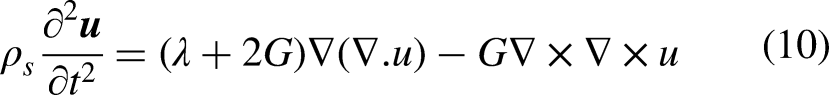
The equation of motion for a linear elastic, homogeneous, isotropic medium is given by:

Using conservation of mass, the instantaneous density,


In addition, it is readily shown that strain tensor,


Using equations (3), (8) and (9), the equation of motion can be rewritten as
Setup of the numerical model
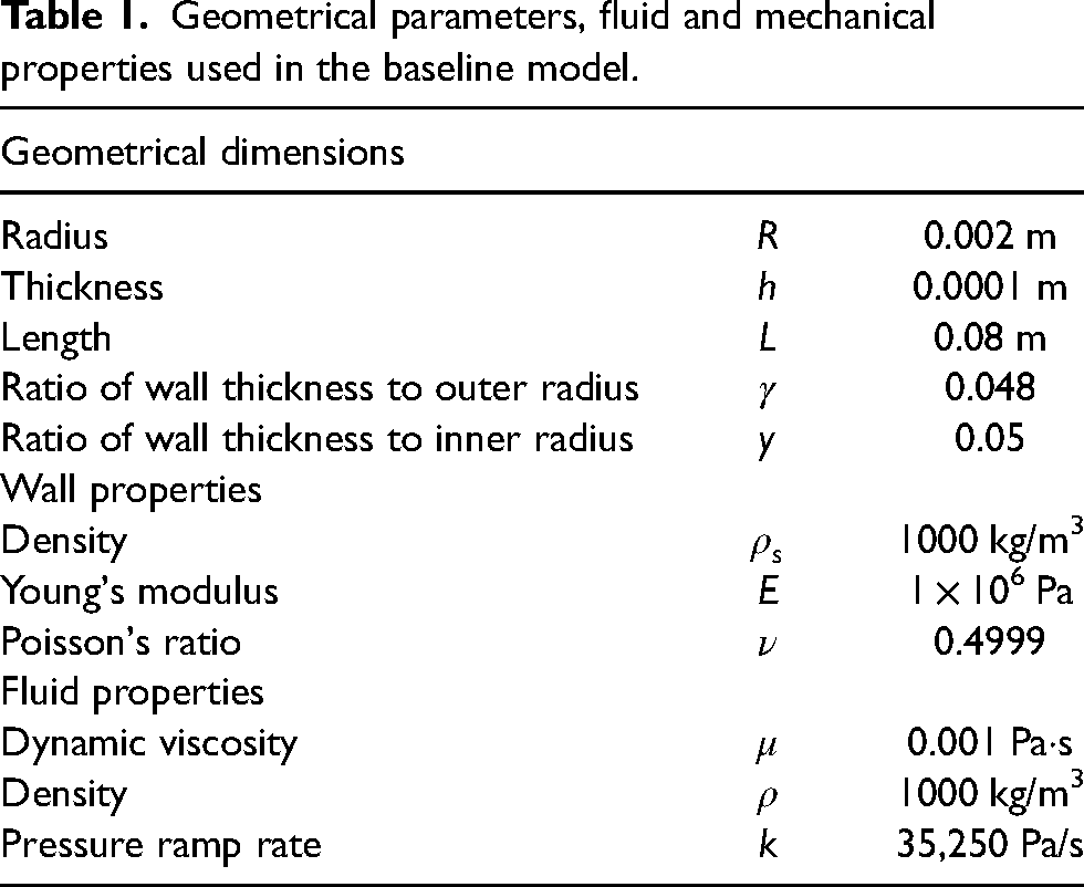
The test case considered is the propagation of a pressure wave along a fluid-filled elastic tube that is subjected to a linear pressure ramp at the inlet. The geometry considered is shown in Figure 1. Details of the geometry and material properties are given in Table 1.

Geometry of the numerical model: showing the fluid region (coloured in blue) and solid region (coloured in orange). The tube is 80 mm long.
Geometrical parameters, fluid and mechanical properties used in the baseline model.
Fluid computational mesh
The fluid model is developed using ANSYS Fluent, version 2021R1. A size control of 0.5 mm is used to generate the mesh in the fluid domain, shown in Figure 2. It has 14,720 nodes and 18,796 cells with three inflation layers. The minimum orthogonal quality of the mesh is 0.72, and the maximum skewness is 0.28. Mesh refinement tests showed this level of mesh refinement to be sufficient.

The computational mesh on the fluid domain.
Fluid boundary conditions and setup
The entrance of the tube is set as a pressure inlet with a linearly increasing pressure applied. The exit is set to a static pressure of 0 Pa. The no-slip condition is applied at the tube wall. A dynamic mesh model is enabled, which allows the shape of the domain to change with time. The diffusion-based smoothing method is chosen to diffuse the boundary motion throughout the interior mesh. The inlet and outlet of the tube are allowed to deform in the planes normal to the axial direction. The tube wall is set as a system coupling zone, which transfers data to and from the structural model.
The second-order implicit transient, pressure-based solver is used to conduct the analysis. The coupled scheme is used, which means the momentum and pressure correction equations are solved in a fully coupled manner. Gradients are determined using the least-squares cell-based option, the pressure is determined using the second-order method, and the second-order upwind scheme is used for the momentum equation. Converged solutions are achieved when the residual values for continuity, x, y and z velocities are below 10–5. The residual values are calculated based on the locally scaled root mean square (RMS) errors.
Mechanical mesh
The choice of meshing strategy is an important component of this study. Of particular interest is an investigation of how the choice of mesh element type affects the solution, particularly in terms of the impact of wall thickness. Three types of elements can be used in Ansys Mechanical to construct the tube: shell, solid, and solid shell. Figure 3 shows the recommended selection criterion, which depends on the aspect ratio, γ, together with a description of the element types.

Shell elements are two-dimensional (2D) and are only suitable for modelling thin structures. In a shell model, the structure is represented by a single plate at the mid-surface. Without the thickness dimension, shell elements cannot achieve precise stress and strain profiles through the wall thickness. Each node of the shell element has six degrees of freedom to compensate for the geometric limitation. In addition to the degrees of freedom in translation, the shell element has degrees of freedom in rotations. Therefore, shell elements can capture the bending behaviour at each node explicitly.
Solid elements are well suited for modelling three-dimensional (3D) thick structures because they can simulate the stress and strain profile through the thickness. However, solid elements cannot capture bending behaviour due to the lack of degrees of freedom in rotations. Shear locking occurs when solid elements are used for thin walls. It means that the structure becomes artificially stiffer than its actual stiffness.
Solid shell elements are designed for simulating thin structures. The solid shell model represents the solid structure using a single-layered solid element. The single-layered solid element allows the model to obtain the stress and strain profile through the thickness. Solid shell elements can overcome shear locking when their thickness is small enough due to their unique kinematic formulations. 22
Different element types are used to build the same model to test their effect. An element size of 0.5 mm is used in all three models. The shell model is represented by a single plate. The solid model has three layers, while the solid shell model only has one. The cross-sectional mesh constructed with different element types are shown in Figure 4 and Table 2 gives details of the number of nodes and elements.

Cross-sectional mesh on the structural domain for a tube thickness of 0.1 mm (a) shell; (b) solid; (c) solid shell.
Mesh statistics for the different structural models.

Mechanical boundary conditions and setup
The inner surface of the wall is set as a fluid–solid interface, which transfers information between the solid and fluid. Axial displacement is constrained in the structure. Large deflections are enabled to allow accurate calculation of the material deformation. The sparse matrix direct solver is used.
Coupling strategy and setup
Ansys System Coupling, version 2021R1, was used to couple the fluid and structural analyses. A two-way data transfer is performed at the interface. The pressure impulse at the inlet causes the fluid to flow along the tube. The force at the fluid interface is then transferred across the structural interface, causing the structural model to deform. The structural displacement information is then transferred back to the fluid domain. This process is continued until convergence is obtained.
The analysis setup for the FSI model is controlled in the System Coupling setup. The duration of the analysis was set as 0.006 s. A timestep of 0.0005 s was selected after assessing the timestep effect upon results. The maximum number of coupling iterations was set to 20, with typically 13 needed for convergence. Quasi-Newton stabilisation was activated to achieve convergence. This method is derived from an interface quasi-Newton coupling algorithm with an approximation for the inverse of the Jacobian (IQN-ILS). 23 The initial relaxation factor applied during the start-up iteration was set to 0.01. The maximum number of time steps to be retained in the Quasi-Newton history was set to one. Data transfers at the interface were deemed to have converged when the globally scaled RMS of the residual values are below 0.01.
Ten cores of Intel(R) Xeon Bronze 3204, @1.90 GHz processor with 64 GB RAM were used to run the model. Two cores were used for the Mechanical solver and eight cores were used for the Fluent solver during the simulation.
Analytical solutions
Wave speed
The transient propagation of fluid flow and stress in a thin-walled elastic tube has been studied by many researchers. The most well-known equation is that of Moens-Korteweg3,4
The assumptions made in the derivation of the equation are: (i) the tube is filled with incompressible and inviscid fluid, (ii) the wall thickness is very small compared with the radius, (iii) the wall material is elastic and isotropic, (iv) the effect of the Poisson's ratio of the wall material is not considered, and (v) the wall only deforms radially.
Bergel
13
modified the Moens-Korteweg equation by including the effect of Poisson's ratio through the wall thickness. This correction compensates for the errors resulting from the thin-wall assumption in the original equation. Although this correction accounts for the effect of the Poisson's ratio, it is still assumed that the length of the tube does not alter, that is, no axial displacement. The modified wave speed becomes

In the derivation of both the Moens-Korteweg equation and Bergel's correction, the elastic tube is not allowed to elongate. The effect of different longitudinal tube constraints was investigated by Wylie et al.
15
The wave speed formulas are modified based on whether longitudinal motion is allowed or not. Different coefficients are used based on the ratio of the wall thickness to the inner radius. When the ratio
For a thin-walled tube, the wave speed is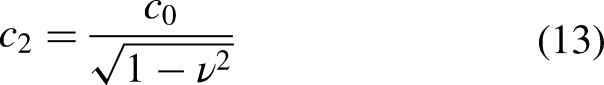

For a thin-walled tube, the wave speed is

Radial displacement
In an elastic tube, when a pressure pulse is applied, the radial displacement along the tube can be calculated using the equation below derived from the analytical solution of Womersley.8,10 However, this equation only applies when the tube is constrained axially.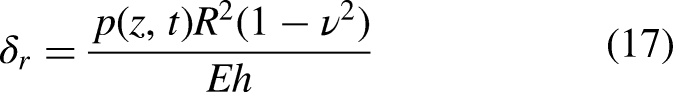
In the simulation, a linearly increasing pressure is applied at the inlet of the fluid domain. The pressure at the inlet follows the following equation:

Effect of fluid compressibility
The fluid is assumed to be incompressible in the Moens-Korteweg equation. By taking the fluid compressibility into account, the wave speed can be calculated using:
5

The density of common fluids is of the order of 103 kg/m3, and the bulk modulus is of the order of 109 kPa. Therefore,
Model verification
Effect of structural element type and wall thickness
The effect of the structural element type is examined by building the same model using different element types. Figure 5 shows the radial mesh displacement along the tube for shell elements. Figure 5(a) shows that the pressure impulse at the inlet increases over time, causing the wall displacement to gradually increase. The simulation is terminated before the wave reaches the end of the tube as it would cause reflections and disturb the profiles. The radial displacement at the inlet over time is recorded and compared with the theoretical results following equation (19). The results show a high level of accuracy for different wall thicknesses.

Propagation behaviour using shell elements: (a) Radial mesh displacements along the tube, (b) Radial displacements at the inlet compared with the analytical solution for various wall thicknesses.
The wave speeds are estimated by calculating the distance travelled by the wave over time. The calculated wave speeds for different structural models are shown in Figure 6. The simulation results from all models are very similar when

The effect of wall thickness on wave speed for different element types.
Mesh and timestep independence studies
A mesh-resolution study was performed by reducing the element size from 0.5 to 0.25 mm. Simulation results are compared against the analytical propagation speed
A timestep independence study in which the timestep was reduced to 0.2 from 0.5 ms also showed the original result to be timestep independent. 1
Effect of wall stiffness
The effect of wall stiffness is examined in the simulations and the results for the propagation speed are compared with the analytical value

The effect of wall stiffness when the tube is constrained axially on: (a) wave speed; (b) radial displacement.
When the tube is constrained axially, axial strain along the tube is zero, while the axial stress varies along the tube. The stress profile matches very well with the assumption of Case (a) from Wylie et al. 15 (see 1 ).
When the tube is free to elongate, the simulated wave speeds are compared with the values for wave speed

The effect of wall stiffness on wave speed when the tube is free to elongate on: (a) wave speed; (b) radial displacement.
Effect of Poisson's ratio
The effect of Poisson's ratio is examined when the tube is constrained axially. Figure 9 shows that as the Poisson's ratio increases, wave speeds from both element types increase, following the trend of the analytic solution yielding the wave speed

The effect of Poisson's ratio when the tube is constrained axially on: (a) wave speed; (b) radial displacement.
When the tube is free to elongate, the Poisson's ratio does not have a significant impact on either the wave speed or the radial displacement. When the Poisson's ratio is increased from 0 to 0.5, the wave speed for both models decreased by only 2%, as can be seen in Figure 10.

The effect of Poisson's ratio when the tube is free to elongate on: (a) wave speed; (b) radial displacement.
Effect of wall material density
In the theoretical PWV calculation, the effect of the added mass, which is the wall mass and the fluid carried with it, is not considered. In the study of Morgan and Ferrante,
7
the effect of solid density was discussed. The study was then extended by Womersley,
10
who examined the effect of mass-loading of the solid. He stated that the wall material density only affects the wave speed if the tube constraint allows longitudinal motion. Womersley
10
defined the term 
If
When the tube is constrained axially, results for the effect of the wall material density are shown in Figure 11. The largest difference between the results is only 3%. Therefore, the wall material density does not have a significant impact on either the wave speed or radial displacement when the tube is constrained axially.

The effect of wall material density when the tube is constrained axially on: (a) wave speed; (b) radial displacement.
When the tube is free to elongate, the wall material density shows an effect on both wave speed and radial displacement, as shown in Figure 12. When the density increases from 1000 to 10,000 kg/m3, the wave speed decreases by around 16%. It also has an impact on the radial displacement. However, the radial displacement at the inlet is almost the same when the density increases from 5000 to 10,000 kg/m3.
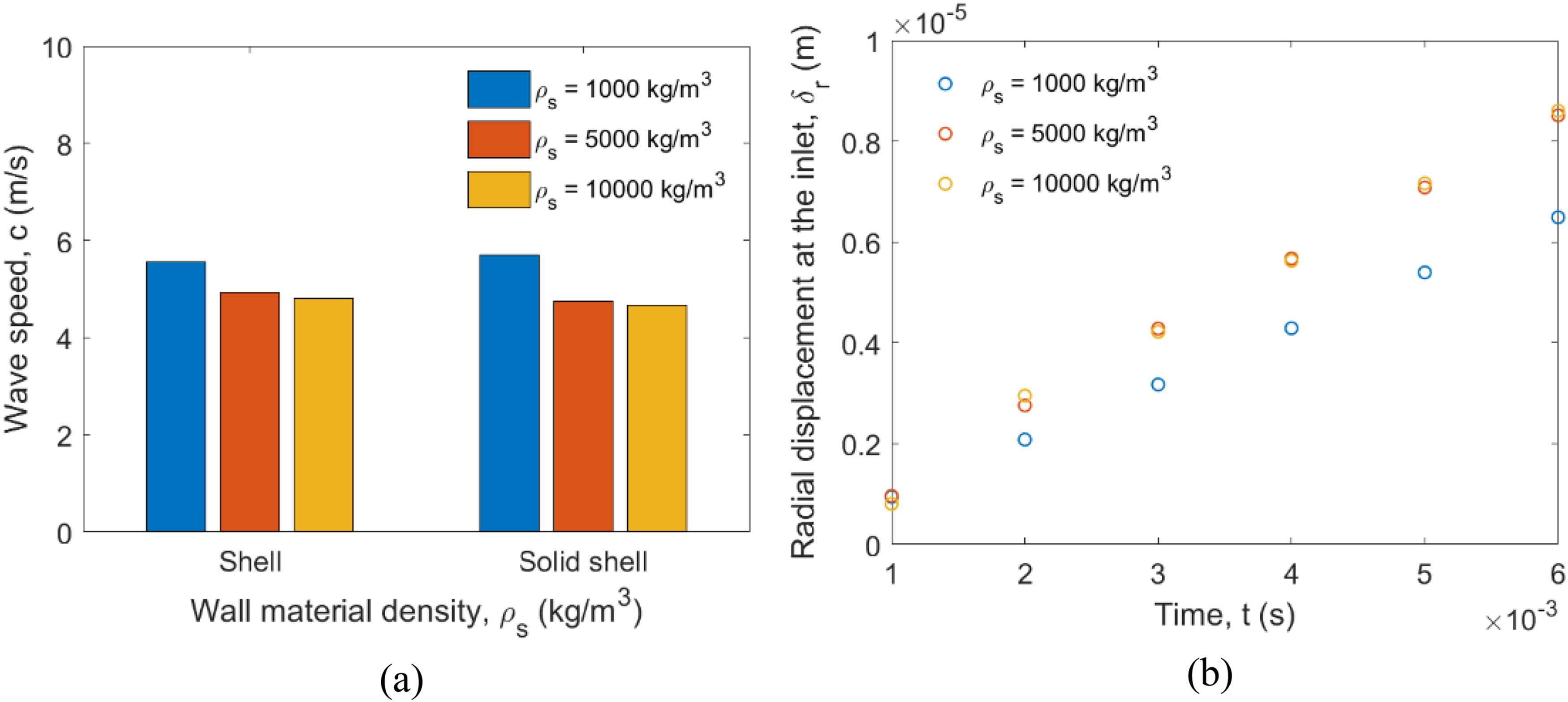
The effect of wall material density when the tube is free to elongate on: (a) wave speed; (b) radial displacement.
The effect of fluid viscosity
The fluid is assumed to be inviscid in the PWV calculation to simplify the equations. However, the fluid viscosity affects the wave velocity significantly according to Womersley 8 and Bergel. 12 In this section, the effect of the fluid viscosity is examined through numerical simulation. As shown in Figure 13, the fluid viscosity has a significant impact on wave speed when the tube is constrained axially. There is a 10% difference when the viscosity is changed from 0.001 to 0.1 Pa·s. However, the radial displacement is independent of the fluid viscosity.
The effect of fluid viscosity when the tube is constrained axially on: (a) wave speed; (b) radial displacement.
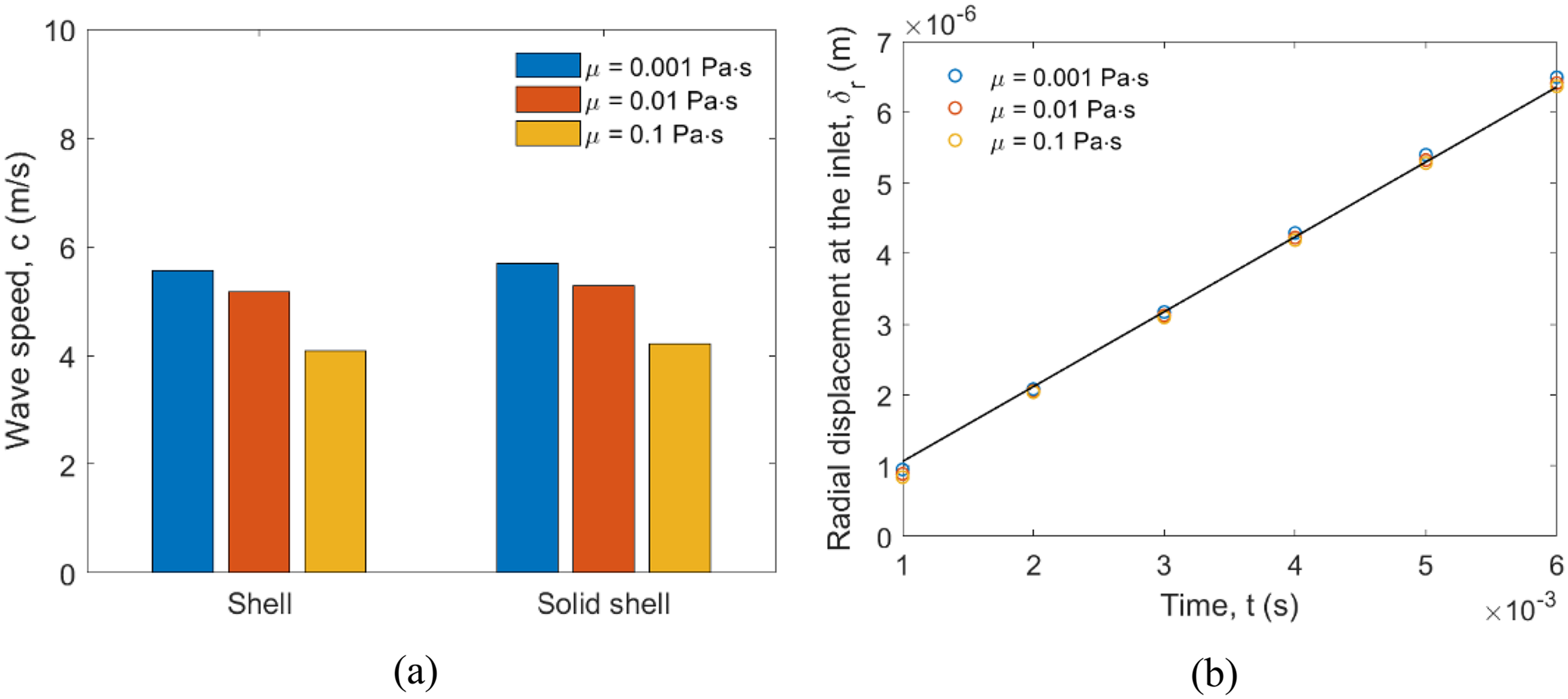
The wave speed is also affected by fluid viscosity when the tube is free to elongate. When the fluid viscosity is increased from 0.001 to 0.1 Pa·s, the wave speed decreases by around 16% as can be seen in Figure 14. Also, the radial displacement decreases when the fluid viscosity increases up to 0.01 Pa.s, and then the effect is small.

The effect of fluid viscosity when the tube is free to elongate on: (a) wave speed; (b) radial displacement.
The effect of pressure ramp rate
The effect of the pressure ramp rate is examined when the tube is constrained axially. As shown in Figure 15, the wave speeds remain the same in both models when the pressure ramp rate changes. The radial displacement results fit perfectly with results from equation (19). Similar behaviour is observed for an unconstrained tube.

The effect of pressure ramp rate when the tube is constrained axially on: (a) wave speed; (b) radial displacement.
Conclusions
Model verification is crucial for simulation development, yet it is often neglected, especially when commercial software is used. In this study, the accuracy of the Ansys System Coupling approach to model FSI of wave propagation in a fluid-filled tube is verified. The choice of structural element type is shown to be important when modelling different wall thicknesses and for moderately thick walls solid shells gave the best results. Specifically, if the ratio of the wall thickness to the tube inner radius is less than 0.1 (y < 0.1), shell elements perform best and above this ratio solid shell or solid elements are required. This corresponds closely with the limit set by Wylie et al. 15 of y < 0.08 for a tube to have thin walls. Where applicable, solid shells are preferred over solids due to their lower computational cost.
As would be expected the tube constraint has an impact on axial stress and strain profiles of the elastic tube material, and this manifests itself in changed wave speeds and wall displacement for different tube materials. This is an important observation, as in many real systems the choice of boundary condition is not obvious. In biomedical systems, there are very few cases where a simple fixed displacement condition can be applied. It is important to examine the sensitivity to both the location of the constraint and the type of boundary condition. This ensures the choice leads to physical results and determines the sensitivity to the condition applied.
Key parameters such as wall thickness and material properties were varied, and results showed excellent agreement with analytical predictions. The simulation results also show the effect of the tube materials, tube constraints and fluid properties, which are not readily available from theoretical studies.
Importantly, it can be concluded that the solution methodology presented here is suitable for the simulation of peristaltic flows that are important in a wide variety of biomedical and engineering simulations. The validation presented here is for a straight tube and demonstrates the accuracy of the FSI coupling methodology used. The same algorithm and methodology can be applied to scans of PWV or other flexible tubes and the same accuracy for properly resolved simulations can be expected. Previous work 25 has shown that the fluid model is very accurate for simulations when a known travelling wave motion is applied to the wall, so the combination of this work and the previous work validates the modelling approach for a wide range of conditions.
Footnotes
Acknowledgements
The authors thank Drs Peter Brand, Luke Mosse and Jindong Yang of LEAP Australia for helpful discussions. XL received an Australian Government Research Training Program Stipend Scholarship and a supplementary scholarship from the Centre for Advanced Food Engineering (CAFE) of the University of Sydney.
Declaration of conflicting interests
The authors declared no potential conflicts of interest with respect to the research, authorship, and/or publication of this article.
Funding
The authors disclosed receipt of the following financial support for the research, authorship, and/or publication of this article: This work was supported by the Medical Research Future Fund (MRFF-ARGCHD000015) and Australian Research Council grant (ARC DP200102164).