A hybrid algorithm for large-scale non-separable nonlinear multicommodity flow problems

Abstract

We propose an approach for large-scale non-separable nonlinear multicommodity flow problems by solving a sequence of subproblems which can be addressed by commercial solvers. Using a combination of solution methods such as modified gradient projection, shortest path algorithm and golden section search, the approach can handle general problem instances, including those with (i) non-separable cost, (ii) objective function not available analytically as polynomial but are evaluated using black-boxes, and (iii) additional side constraints not of network flow types. Implemented as a toolbox in commercial solvers, it allows researchers and practitioners, currently conversant with linear instances, to easily manage large-scale convex instances as well. In this article, we compared the proposed algorithm with alternative approaches in the literature, covering both theory and large test cases. New test cases with non-separable convex costs and non-network flow side constraints are also presented and evaluated. The toolbox is available free for academic use upon request.

Introduction

The importance of network flow problems has been demonstrated in many successful real-world applications. ¹ Underlying network structures are also found in a great variety of large-scale optimization problems ranging from transportation, power grids, communications, supply chains to social networks.

While earlier works in network flow problems focus on linear instances, ² it has been recognized that real-world situations can easily lead to nonlinearities due to physical phenomena and economic considerations.^3,4 Indeed, as more applications look more complicated planning problems such as those dealing with uncertainties, disruption, and sabotage, convex instances arise. For example, separable convex cost functions are considered by Dembo and Klincewicz, ⁵ Bertsekas et al., ⁶ Babonneau and Vial, ⁷ and Bertsekas et al. ⁸ However, it has also been reported that separable costs are not realistic representations of real traffic networks, ⁹ and possibly non-separable, non-convex functions. ³ Moreover, separable convex network flow problems are not much harder than linear optimization problems ¹⁰ while general non-separable optimization problems have been shown to be considerably more difficult than separable problems. ¹¹

Although such research works of non-separable costs are not much in the literature, their applications are often encountered in many transportation networks. For example, considering a two-way road ¹² travel cost depends not only on traffic volume traveling in its direction but also on traffic volume in the opposite direction. Other example in urban transportation networks, travel cost on a link depends on congestion occurring at intersections since traffic volumes increase at the intersecting links. Akcelik ¹³ introduced non-separable travel cost functions to estimate the capacity of a shared lane at a signalized intersection. Larsson et al. ¹⁴ refined conventional non-separable and typically asymmetric strategy on a traffic equilibrium assignment model. Agustin et al. ¹⁵ proposed an air traffic flow management model for flight cancelation and rerouting with separable and non-separable ground holding and air delay costs. Gabriel and Bernstein ¹⁶ introduced some non-separable nonlinear route costs in (i) nonlinear valuation of travel time: the small amount of time has relatively low value whereas the large amount of time varies valuable, (ii) non-separable tolls and fares: toll roads and transit systems have non-separable toll/fare structure, and (iii) emission fares: emissions of hydrocarbons and carbon monoxide are a nonlinear function of travel times. Hence, non-separable convex cost networks as well as their solution methods are very important and need to be investigated carefully. Recently, Meselhi et al. ¹⁷ has investigated large-scale optimization problems with the objective function of non-separable costs, and proposed three different strategies for handling overlapping variables to reduce overlapping among sub-problems. However, this model did not consider multicommodity and a set of constraints in the optimization problems. Hence, their approach could not handle general problem instances and not be easily applied for industrial applications. Consequently, there is little insight into the behavior of network flow optimal solutions in the presence of such non-separable costs.

In addition, the open-source codes of the existing solution methods for network flow problems with separable/non-separable convex cost are not readily available, or specialized codes ² are restricted to a small group of researchers. Those involved in large-scale network problems do not have resources for algorithmic developments. We plan to fill the gap. In fact, in theory, these problems can be solved by general nonlinear programing techniques. Nevertheless, optimization methods based on exploring their special structure make it much more attractive and especially get advantages of computation time. We may achieve efficiency by solving sub-problems for which polynomial algorithms, such as shortest path. ²

In this article, we introduce an efficient hybrid algorithm (namely, CMNET) for solving large-scale non-separable convex network flow problems. This method is a combination of gradient projection, shortest path algorithm, and golden section search with the advantages of convergence property and efficient computation time. In addition to our main contribution of solving such non-separable convex network flow problems, our approach can handle the problems with objective functions that are not available analytically as polynomial but can be evaluated using black-boxes. Moreover, it can solve the network flow problems including additional side constraints (i.e. non-network flow types).

The remainder of this article is organized as follows. A detailed description of network flow problems with generalized non-separable convex costs is provided in section ‘Multicommodity flows with non-separable nonlinear costs’. In this section, we also introduce the generalized formulation of the non-separable network flow problems. Section ‘CMNET’ presents the two-phase projected gradient algorithm proposed, as well as its convergence. Section ‘Computational results’ describes the computational experiments to illustrate the efficiency of the proposed algorithm. The experiments include a comparison with analytic center cutting plane method (ACCPM), ⁷ an implementation of a constrained ACCPM to solve nonlinear multicommodity flow problems, on separable instances, and the performance evaluation of our algorithm on non-separable instances are presented. Finally, conclusions and future work are summarized in section ‘Conclusions and future work’.

Multicommodity flows with non-separable nonlinear costs

Definition of the problem

Assumption

We only investigate non-separable multicommodity flow problems with continuously differentiable convex objective function.

General formulation

Let $\mathcal{G}=(\mathcal{N},\mathcal{A})$ be a directed graph with the number of nodes $n:=|\mathcal{N}|$ and the number of arcs $a:=|\mathcal{A}|$ . Then, we denote $\mathbf{H}\in {\mathrm{R}}^{n\times a}$ to be the node-arc incidence matrix of $\mathcal{G}$ . Let $K$ be the number of commodities to be transported through the network. For each commodity $k$ , there is an amount of demand $d^k$ required to deliver from source node $s_k$ to destination node $t_k$ . Incorporating multicommodity into the network flow problem increases significantly the size of problem due to the additional number of decision variables and constraints. The general non-separable nonlinear multicommodity flow problem (NNMFP) can be formulated by

$\mathbf{[}\mathbf{N}\mathbf{N}\mathbf{M}\mathbf{F}\mathbf{P}\mathbf{]}:$

${\min }_x$	$g(x)$
s.t.	$\mathbf{H}{x}^k=d^k{\delta }^k,\mathrm{\forall }k\in \mathcal{K}$ ,
	$\sum _{k\in \mathcal{K}}{x}_{ij}^k\le c_{ij},\mathrm{\forall }(i,j)\in \mathcal{A}$ ,
	$x_{ij}^k\ge 0,\mathrm{\forall }k\in \mathcal{K},(i,j)\in \mathcal{A}$ ,

where

$g(x)$	is a continuously differentiable non-separable convex objective function,
$x$	is a decision vector with the components $x_{ij}^k$ , $\mathrm{\forall }k\in \mathcal{K},(i,j)\in \mathcal{A}$ ,
$x^k$	denotes the $a$ -dimension flow vector of commodity $k$ ,
$c_{ij}$	is the flow capacity on arc $(i,j)$ ,
${\delta }^k$	is the $n$ -dimension vector with the components ${\delta }_j^k,\mathrm{\forall }j\in \mathcal{N}$ determined by

$${\delta }_j^k=\{\begin{array}{ccc}1& \text{if}& s_k=j\\ -1& \text{if}& t_k=j\\ 0& & \text{otherwise}\end{array}$$

(1)

Congestion and propagation functions

Convex objective functions investigated in this article are often encountered in many real-life applications. For example, congestion functions pose generalized convex cost in network flow problems. Various types of such congestion functions can be found:

Traffic assignment manual ¹⁸

Link capacity functions: A review ¹⁹

Improved speed-flow relationships: Application to transportation planning models. ²⁰

However, propagation functions which pose non-separable cost in network flow problems have not considered appropriately. In the literature, there are a few works relevant to such functions. They arose mainly from traffic assignment problems. For example, Gabriel and Bernstein ¹⁶ introduced some non-separable route costs caused by tolls and fares.

Practical applications

Network flow problems with non-separable nonlinear costs are often encountered in logistics and supply chain management (i.e. multicommodity flows). In addition, such problems also arise in the fields of transportation and telecommunications.

Transportation problems

In general, transportation problems with non-separable cost are different from ordinary network flow problems. Caused by tolls and fares, these transportation problems have to be formulated in the route-flow space. Hence, they cannot be solved using the traditional link-based algorithms, such as the Frank-Wolfe algorithm. ²¹ Also, the diagonalized methods do not work well on the non-additive problems since the diagonalized subproblems are poor approximations of the original problem. Two types of transportation problems include ⁹ :

Traffic equilibrium problem is to find the traffic-flow pattern by allocating the origin–destination demands to the traffic network such that all used routes between each origin–destination pair have equal and minimum travel cost, and no unused route has lower travel cost than minimum travel cost.

Traffic assignment problem is to allocate a given set of trip/route interchanges to a certain transport network. The solution of the assignment problem includes an estimate of the traffic volumes and the corresponding travel times or costs on each arc of the transport network.

Telecommunications

Such network flow problems with non-separable nonlinear costs are also encountered in the field of telecommunications, that is, data networks, where we have to transmit data appropriately to satisfy the demands of hubs in the network. ²² In addition, in telecommunication applications there are usually additional time-delay or reliability requirements on paths, which may cause non-separable cost as well as side constraints on paths. ²³

Importance of non-separable nonlinear costs and side constraints

Node congestion/junction effect/delay propagation

Non-separable cost is often encountered in traffic assignment models where two-way traffic is considered. ¹² Then, traffic time/cost depends not only on traffic volume traveling in this direction but also on traffic volume in the opposite direction. Furthermore, in urban transportation networks, travel time/cost on a link depends on delays occurring at intersections or traffic volumes on the intersecting links. As a result, travel time/cost on precedent and/or successive links is also affected, which leads to delay propagation in transport networks.

Side constraints

This problem includes flow capacity and conservation (network) constraints and other additional (non-network) constraints, aka side constraints. There is a few studies devoted to side constrained network models. In the traffic assignment problem, researchers mainly investigate the link capacity as the side constraints. ⁹ In the traffic equilibrium problem, side constraints may be caused by (i) the effects of a traffic control policy, (ii) the refinement strategies, and (iii) the flow restrictions that a central authority wishes to impose upon the users of the network. ¹⁴ In telecommunication applications, side constraints causing time-delay or reliability requirements on paths were investigated by Holmberg and Yuan. ²³

CMNET

CMNET is a toolbox of the commercial solvers (e.g. CPLEX), which is constructed on a two-phase gradient projection algorithm. The proposed algorithm is a combination of gradient projection, shortest path formulation and golden section search for solving large-scale non-separable nonlinear multicommodity flow problems. In this section, after describing the details of the two-phase gradient projection algorithm, we provide the optimal properties of this algorithm and its convergence rate. Next, the importance of a commercial solver add-on is discussed.

Two-phase gradient projection algorithm

At each iteration in the proposed algorithm, we solve the sequence of the following subproblems: linearized problem (LP) and second-order conic programing (SOCP). The linearized multicommodity flow problem can be formulated by

$\mathbf{[}\mathbf{L}\mathbf{P}\mathbf{]}:$

${\min }_x$	${\displaystyle \sum _{(i,j)\in \mathcal{A}}\sum _{k\in \mathcal{K}}{g}_{ij}(x_{ij}^k)}$
s.t.	$\mathbf{H}{x}^k=d^k{\delta }^k,\mathrm{\forall }k\in \mathcal{K}$
	$x^k\ge 0,\mathrm{\forall }k\in \mathcal{K}$

where $g_{ij}(x_{ij}^k)$ is a linear cost objective function. $g_{ij}(x_{ij}^k)=t_{ij}{x}_{ij}^k$ is only used at the initialization step, otherwise $g_{ij}(x_{ij}^k)=\frac{\mathrm{\partial }g(x)}{\mathrm{\partial }{x}_{ij}}$ .

Let $\mathbf{X}$ be the feasible solution set of network flow problem considered. SOCP at iteration $h+1$ in CMNET can be formulated by

$\mathbf{[}\mathbf{S}\mathbf{O}\mathbf{C}\mathbf{P}\mathbf{]}:$

$${\min }_{x\in \mathbf{X}}\Vert z_{h+1}-x{\Vert }_2^2$$

where $z_{h+1}$ is a scalar vector, out of feasible solution space, determined by $z_{h+1}:=x_h-{\beta }_h\mathrm{\nabla }g(x){|}_{x=x_h}$ .

In addition, we use the golden section search to find a solution improvement at each iteration. We illustrate the basic implementation of this proposed algorithm at iteration $h+1$ in Figure 1.

Figure 1.

Illustration of one iteration in the two-phase gradient projection algorithm.

Descent direction from the shortest path (SP)

Dijkstra’s algorithm which was firstly introduced by Dutch computer scientist Edsger Dijkstra ²⁴ is a graph-based search algorithm. In the literature, this algorithm has been applied for searching the SPs from a source to a destination on a graph with non-negative arc costs. In the two-phase gradient projection algorithm, instead of solving the LP by commercial solvers we used Dijkstra’s algorithm as a subroutine for determining the transport path with the lowest cost between a supply and a customer. For the multicommodity flow problems where each commodity has a pair of supply–demand nodes, we repeatedly use Dijkstra’s algorithm to find the corresponding lowest cost paths. To save the computation time, we solve the commodities with the same supply nodes at the same moment. A parallel computing strategy with a number of CPU cores can be applied to improve the efficiency of the procedure.

A modified gradient projection method with $\beta$ adjustment strategy

We develop the two-phase gradient projection algorithm based on the gradient projection method introduced by Bertsekas. ²⁵ The optimal properties of this hybrid algorithm are thus still maintained as that of the standard gradient projection method. However, to improve the convergent rate we propose an efficient stepsize adjustment strategy, where value ${\beta }_h$ at iteration $h+1$ reduces if solution $x_{h+1}^{SOCP}$ obtained by solving the SOCP does not satisfy one of the following conditions:

Improvement condition:

$$g(x_{h+1}^{SOCP})<g(x_h)$$

(2)

Local search condition:

$$\mathrm{\nabla }g{(x)}^{\prime }{|}_{x=x_{h+1}^{SOCP}}(x_h-x_{h+1}^{SOCP})<0$$

(3)

Then, the SOCP is resolved with an updated value ${\beta }_h$ . This procedure terminates if condition (2) or (3) is satisfied.

In addition, if value $cosine$ made by two vectors $-\mathrm{\nabla }g(x){|}_{x=x_{h+1}^{SOCP}}$ and $z_{h+1}-x_{h+1}^{SOCP}$ at iteration $h+1$ decreases as compared with that at the previous iteration $h$ , value $\beta$ is reduced in the next iteration. This may help obtain solutions with larger value $cosine$ in the next iterations, and then the convergence rate is improved. In the implementation of the algorithm, $\beta$ decrement factor is set to be 0.1, while the corresponding factor in decreasing $\beta$ at the SOCP is 0.5.

Golden section search (GSS)

The GSS is a technique for finding the minimal or maximal points of a strictly unimodal function. These points are found by successively limiting the range of values inside that the points are known to exist. ²⁶ In the CMNET, GSS is used to determine the improved solution between the implements of SP, as well as after solving the SOCP where local search condition 3 is satisfied.

Termination criterion

In convex optimization problem, the gradient vector of optimal solution makes an angle ${90}^{\circ }$ with the tangent hyperplane at that solution point. Based on this viewpoint, we propose a new termination criterion for stopping the algorithm. The algorithm stops when value $cosine$ made by two vectors $-\mathrm{\nabla }g(x){|}_{x=x_{h+1}^{SOCP}}$ and ( $z_{h+1}-x_{h+1}^{SOCP}$ ) at iteration $h+1$ is large enough:

$$cosine:=\frac{(-\mathrm{\nabla }g(x){|}_{x=x_{h+1}^{SOCP}}{)}^{\prime }(z_{h+1}-x_{h+1}^{SOCP})}{\Vert -\mathrm{\nabla }g(x){|}_{x=x_{h+1}^{SOCP}}{\Vert }_2\Vert z_{h+1}-x_{h+1}^{SOCP}{\Vert }_2}\ge (1-ϵ)$$

(4)

where $ϵ$ is a small positive scalar. Figure 2 illustrates the termination.

Figure 2.

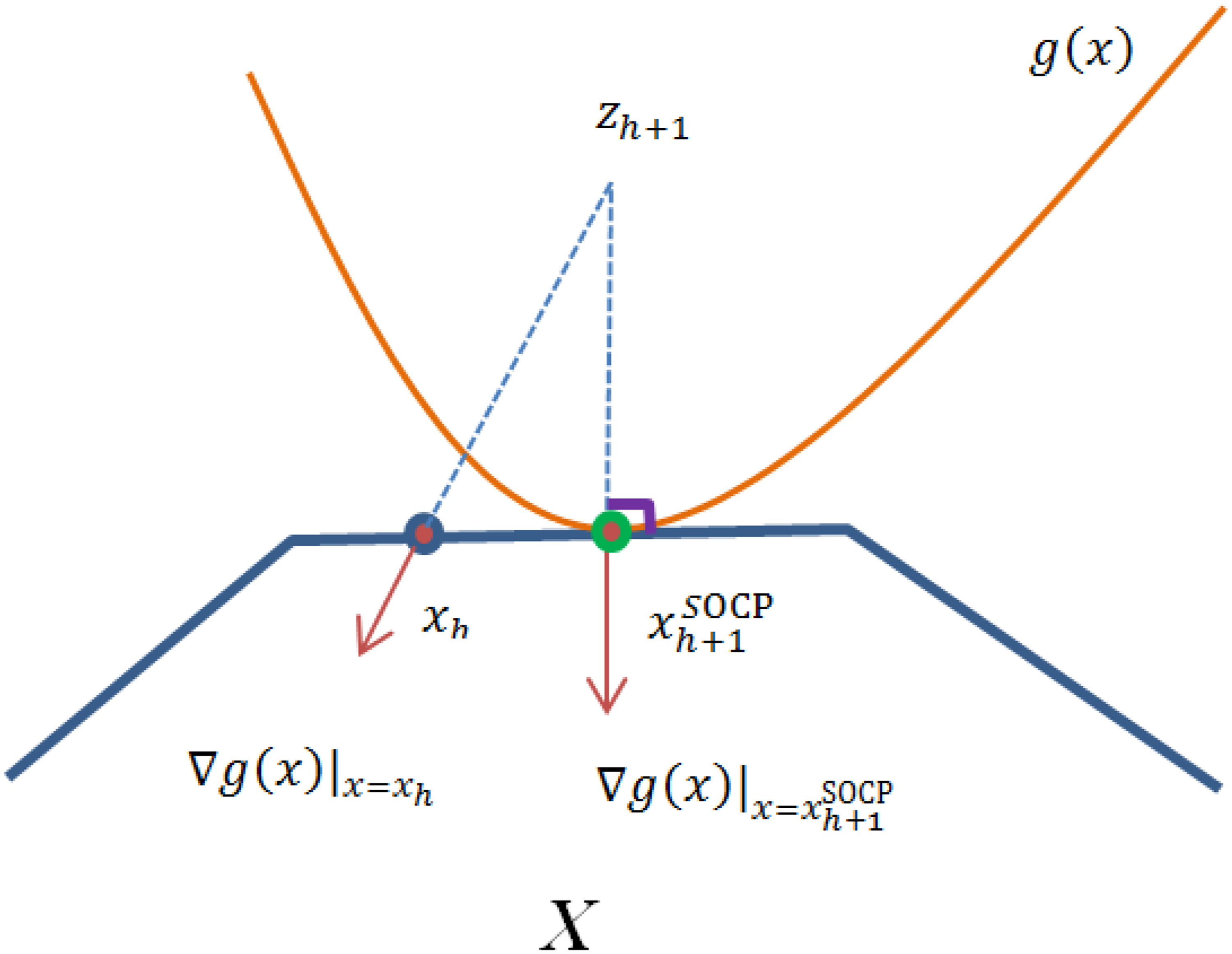
Illustration of termination criterion of the two-phase gradient projection algorithm.

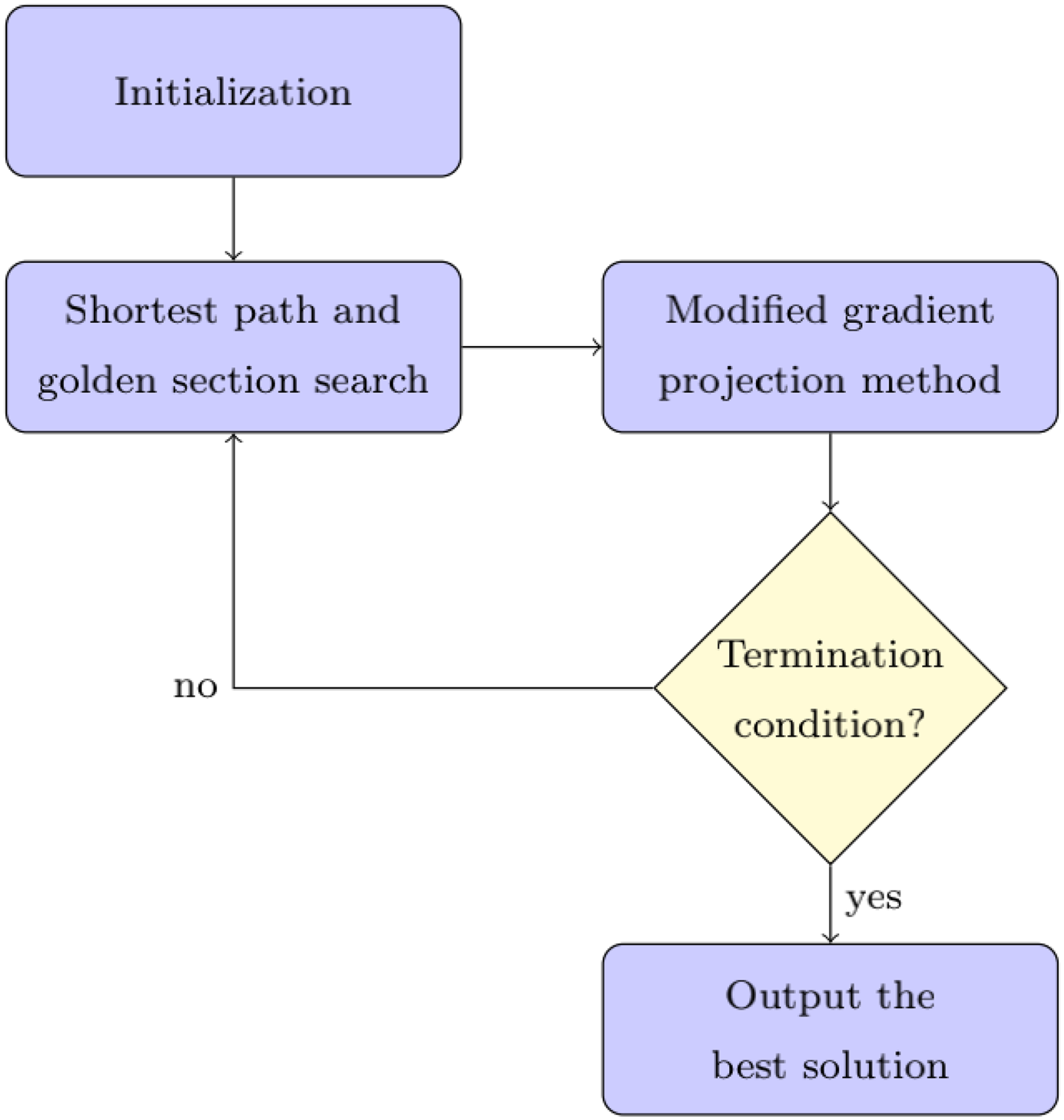
Pseudo code and flowchart

A pseudo code of the two-phase gradient projection algorithm is shown in Algorithm 1. A flowchart of this algorithm is shown in Figure 3. The algorithm is a hybrid of gradient projection with SP and GSS. Hence, its computational complexity is $O(n^2+log(1/\epsilon ))$ .

Algorithm 1.

$\mathbf{S}\mathbf{t}\mathbf{e}\mathbf{p}\mathbf{0.}$	$\mathbf{I}\mathbf{n}\mathbf{i}\mathbf{t}\mathbf{i}\mathbf{a}\mathbf{l}\mathbf{i}\mathbf{z}\mathbf{a}\mathbf{t}\mathbf{i}\mathbf{o}\mathbf{n}:$
	Set $h:=0$ , $ϵ:=1\times {10}^{-8}$ , and ${\beta }_0:=1000$ .
	Let $x_0$ be the initial decision vector arbitrarily chosen. In this paper, we used dijkstra’s algorithm 24 to solve shortest paths subproblem with linear cost $t_{ij}$ at each arc $(i,j)$ to find $x_0$ .
$\mathbf{S}\mathbf{t}\mathbf{e}\mathbf{p}\mathbf{1.}$	$\mathbf{S}\mathbf{h}\mathbf{o}\mathbf{r}\mathbf{e}\mathbf{s}\mathbf{t}\mathbf{p}\mathbf{a}\mathbf{t}\mathbf{h}\mathbf{a}\mathbf{n}\mathbf{d}\mathbf{G}\mathbf{S}\mathbf{S}:$
	Solve a sequence of shortest paths subproblems with linear cost $\frac{\mathrm{\partial }g(x)}{\mathrm{\partial }{x}_{ij}}{|}_{x=x_h}$ at each arc $(i,j)$ and apply GSS to find an improved solution between two implementations of solving the shortest path subproblems. The procedure is repeated 50 times to find $x_{h+1}$ , and let ${\beta }_{h+1}:={\beta }_h$ , $h:=h+1$ .
$\mathbf{S}\mathbf{t}\mathbf{e}\mathbf{p}\mathbf{2.}$	$\mathbf{M}\mathbf{o}\mathbf{d}\mathbf{i}\mathbf{f}\mathbf{i}\mathbf{e}\mathbf{d}\mathbf{g}\mathbf{r}\mathbf{a}\mathbf{d}\mathbf{i}\mathbf{e}\mathbf{n}\mathbf{t}\mathbf{p}\mathbf{r}\mathbf{o}\mathbf{j}\mathbf{e}\mathbf{c}\mathbf{t}\mathbf{i}\mathbf{o}\mathbf{n}:$
	Solve the $\mathbf{S}\mathbf{O}\mathbf{C}\mathbf{P}$ with $z_{h+1}:=x_h-{\beta }_h\mathrm{\nabla }g(x){|}_{x=x_h}$ .
	$\mathbf{I}\mathbf{f}$ satisfying one of the following conditions:
	$g(x_{h+1}^{SOCP})<g(x_h)$ or $\mathrm{\nabla }g{(x)}^{\prime }{|}_{x=x_{h+1}^{SOCP}}(x_h-x_{h+1}^{SOCP})<0$ ,
	$\mathbf{T}\mathbf{h}\mathbf{e}\mathbf{n}$ go to Step\, 3,
	$\mathbf{E}\mathbf{l}\mathbf{s}\mathbf{e}$ reduce $\beta$ a half, and go back Step 2.
$\mathbf{S}\mathbf{t}\mathbf{e}\mathbf{p}\mathbf{3.}$	$\mathbf{C}\mathbf{h}\mathbf{e}\mathbf{c}\mathbf{k}\mathbf{t}\mathbf{e}\mathbf{r}\mathbf{m}\mathbf{i}\mathbf{n}\mathbf{a}\mathbf{t}\mathbf{i}\mathbf{o}\mathbf{n}\mathbf{c}\mathbf{o}\mathbf{n}\mathbf{d}\mathbf{i}\mathbf{t}\mathbf{i}\mathbf{o}\mathbf{n}:$
	$\mathbf{I}\mathbf{f}$ satisfying the termination criterion (4),
	$\mathbf{T}\mathbf{h}\mathbf{e}\mathbf{n}$ stop and conclude that $x_{h+1}^{SOCP}:=\arg {\min }_{x\in \mathbf{X}}g(x).$
	$\mathbf{I}\mathbf{f}$ $\mathrm{\nabla }g{(x)}^{\prime }{|}_{x=x_{h+1}^{SOCP}}(x_h-x_{h+1}^{SOCP})<0$ ,
	$\mathbf{T}\mathbf{h}\mathbf{e}\mathbf{n}$ implement GSS to find an improved solution $x_{h+1}^{GSS}$ between $x_h$ and $x_{h+1}^{SOCP}$ .
	Let $h:=h+1$ , and go back Step 1.

Figure 3.

Flowchart of the two-phase gradient projection algorithm.

Strategies to reduce computation memory and improve CMNET’s performance

For computation time, we used Dijkstra’s algorithm to search the lowest cost paths for commodities with the same supply nodes simultaneously.

WIN64 is used to capture the advantage of unlimited RAM memory.

Only non-zero values of decision variable during the solution procedure are recorded to save the memory of CPU.

To save the memory of CPU for solving the SOCP in Step 2 by CPLEX, we solved such subproblem with each commodity $k$ independently:

$\mathbf{[}\mathbf{i}\mathbf{n}\mathbf{d}\mathbf{i}\mathbf{v}\mathbf{i}\mathbf{d}\mathbf{u}\mathbf{a}\mathbf{l}\mathbf{S}\mathbf{O}\mathbf{C}\mathbf{P}\mathbf{]}:$

${\min }_{x^k}$	$\Vert z_{h+1}^k-x^k{\Vert }_2^2$
s.t.	$\mathbf{N}{x}^k=d^k{\delta }^k,$
	$x^k\ge 0$

• where $z_{h+1}^k:=x_h^k-{\beta }_h\mathrm{\nabla }g(x){|}_{x=x_h^k}$ .

• Similarly, when using the GSS to find the best solution between two vectors $x_h$ and $x_{h+1}$ , we perform the searching process on two corresponding vectors $y_h$ and $y_{h+1}$ , where $\sum _{k\in \mathcal{K}}{x}_h^k=y_h$ .

Optimality properties

Convergence analysis

In section ‘Two-phase gradient projection algorithm’, if the optimal solution is an extreme point, the CMNET can obtain this solution as satisfying Proposition 1.

Proposition 1

Given that $x^{*}$ occurs at an extreme point of $\mathbf{X}$ , $x_h$ is the global optimal solution of $\mathbf{(}\mathbf{N}\mathbf{N}\mathbf{M}\mathbf{F}\mathbf{P}\mathbf{)}$ if and only if $x_{h+1}=x_h$ .

Proof

If $x_h:=\arg {\min }_{x\in \mathbf{X}}g(x)$ , then $\mathrm{\nabla }g(x{)}_{x=x_h}^{\prime }(x-x_h)\ge 0,\mathrm{\forall }x\in \mathbf{X}.$

We have $x_{h+1}:=\arg {\min }_{x\in \mathbf{X}}{\mathrm{\nabla }g(x){|}_{x=x_h}}^{\prime }x.$

Because of the unique solution, $x_{h+1}=x_h.$

To obtain a contradiction, assume that

$\mathrm{\exists }x\in \mathbf{X},x\ne x_h:{\mathrm{\nabla }g(x){|}_{x=x_h}}^{\prime }(x-x_h)<0.$

Then, ${\mathrm{\nabla }g(x){|}_{x=x_h}}^{\prime }x<{\mathrm{\nabla }g(x){|}_{x=x_h}}^{\prime }{x}_h.$

When $\mathbf{(}\mathbf{L}\mathbf{P}\mathbf{)}$ is solved, if $x_{h+1}=x_h$ , then ${\mathrm{\nabla }g(x){|}_{x=x_h}}^{\prime }x<{\mathrm{\nabla }g(x){|}_{x=x_h}}^{\prime }{x}_{h+1}$ , which is contradicted since $x_{h+1}:=\arg {\min }_{x\in \mathbf{X}}{\mathrm{\nabla }g(x){|}_{x=x_h}}^{\prime }x$ .

Hence, when $x_{h+1}=x_h$ , not $\mathrm{\exists }x\in \mathbf{X},x\ne x_h:{\mathrm{\nabla }g(x){|}_{x=x_h}}^{\prime }(x-x_h)<0$ .

In other words, this completed the proof.

In section ‘Two-phase gradient projection algorithm’, in the case where the optimal solution is on the boundary of feasible solution set, the CMNET can obtain this solution as the termination condition is satisfied according to Proposition 2.

Proposition 2

Given that $z_{h+1}:=x_h-{\beta }_h\mathrm{\nabla }g(x){|}_{x=x_h}$ , where ${\beta }_h$ is a positive stepsize corresponding to the $\beta$ adjustment strategy in the CMNET; and $x_{h+1}^{SOCP}:=\arg {\min }_{x\in \mathbf{X}}\Vert z_{h+1}-x{\Vert }_2^2$ . If

$$\frac{(-\mathrm{\nabla }g(x){|}_{x=x_{h+1}^{SOCP}}{)}^{\prime }(z_{h+1}-x_{h+1}^{SOCP})}{\Vert -\mathrm{\nabla }g(x){|}_{x=x_{h+1}^{SOCP}}{\Vert }_2\Vert z_{h+1}-x_{h+1}^{SOCP}{\Vert }_2}\ge (1-\epsilon )$$

with $\epsilon$ is a sufficient small positive scalar, then $x_{h+1}^{SOCP}:=\arg {\min }_{x\in \mathbf{X}}g(x)$ .

Proof.

We say that a solution $x^{*}\in \mathbf{X}$ is the global optimal solution of the convex network problem if and only if it satisfies the first-order condition for optimality

$$\mathrm{\nabla }g{(x)}^{\prime }{|}_{x=x^{*}}(x-x^{*})\ge 0,\mathrm{\forall }x\in \mathbf{X}$$

(5)

In other words, $\mathrm{\nabla }g{(x)}^{\prime }{|}_{x=x^{*}}$ makes an angle ${90}^{\circ }$ with the tangent hyperplane at $x^{*}$ .

From the definition of $x_{h+1}^{SOCP}$ as the projected solution on $\mathbf{X}$ of $z_{h+1}$ :

$$x_{h+1}^{SOCP}:=\arg {\min }_{x\in \mathbf{X}}\Vert z_{h+1}-x{\Vert }_2^2$$

we have

$${[z_{h+1}-x_{h+1}^{SOCP}]}^{\prime }[x-x_{h+1}^{SOCP}]\le 0,\mathrm{\forall }x\in \mathbf{X}.$$

(6)

Here, $(z_{h+1}-x_{h+1}^{SOCP})$ is orthogonal to the tangent hyperplane at $x_{h+1}^{SOCP}$ .

From (5) and (6), we can say that

$$x_{h+1}^{SOCP}:=\arg {\min }_{x\in \mathbf{X}}g(x)$$

with the condition of

$$\frac{(-\mathrm{\nabla }g(x){|}_{x=x_{h+1}^{SOCP}}{)}^{\prime }(z_{h+1}-x_{h+1}^{SOCP})}{\Vert -\mathrm{\nabla }g(x){|}_{x=x_{h+1}^{SOCP}}{\Vert }_2\Vert z_{h+1}-x_{h+1}^{SOCP}{\Vert }_2}\ge (1-\epsilon )$$

Therefore, this completed the proof.

Under Proposition 2 and that { $x_k$ } is a sequence generated by solving the SOCP and SP where ${\beta }_k$ is updated according to the $\beta$ adjustment strategy, we always obtain

$$f(x_{k+1})\le f(x_k),\mathrm{\forall }k$$

(7)

Then, every limit solution of { $x_k$ } is a stationary point.

Convergence to local minima of non-convex multicommodity flow problems

In theory, we may divide a non-convex function into a combination of quasi-convex functions considering decision variables a bounded range. Hence, based on the convergence property of the CMNET for solving convex multicommodity flow problems discussed in the section, the CMNET can find the local minima.

Importance of a commercial solver add-on

Commercial solvers (e.g. CPLEX) have been widely used by researchers and practitioners for solving LP problems as well as convex quadratically constrained problems. The performance of such solvers is proven by many successfully practical applications. However, the solvers may not solve generalized convex optimization problems, which are often encountered in real-life. Hence, based on the efficiency of the solvers to develop a solver add-on is very important. This not only makes an inheritable powerful solver add-on, but also the fundamental to build other add-ons.

Computational results

The major goal of our computational experiments is to evaluate the efficiency of the CMNET for solving test cases with (i) non-separable convex costs and (ii) additional side constraints. Commercial solvers for convex or non-convex optimization can only solve the small-scale instances, while our paper investigates the large-scale instances. Hence, we did not make the comparison with such commercial solvers. To compare our algorithm with ACCPM, ⁷ an algorithm for separable convex network flow problems, we firstly carry out the experiments on test cases with separable convex costs.

We developed the CMNET in Visual C++, and performed the experiments on a PC (Intel Core i5-2500 CPU 3.30 GHz, RAM 16.0 GB) under Windows 7 operating system.

All instances were solved by the CMNET with parameter settings:

Initial ${\beta }_0=1000$

Termination condition $ϵ=1\times {10}^{-5}$ or $1\times {10}^{-8}$ (to compare the computational time and the solution quality, respectively). In addition, after 1000 iterations, if the termination condition is not met, the program will stop and report the best solution found.

SOCP termination = $1\times {10}^{-11}$

$\beta$ down factor = 0.5

$\beta$ down factor cosine = 0.1

Number of SP iterations per SOCP = 50

Number of GSS iterations = 20

CPX_PARAM_BARSTARTALG = 3: Barrier starting point algorithm (i.e. average of primal estimate, dual 0 (zero)) is used

CPX_PARAM_BARCOLNZ = 3: Number of nonzero entries that make a column dense

CPX_PARAM_PREIND = 0: Switch off presolving

CPX_PARAM_DEPIND = 0: Turn off dependency checking

In addition to using the pure solution quality and computation time to compare the performance of the CMNET and the ACCPM, we use $ratio$ and $relativegap$ as performance measures. These measures are calculated as follows:

$$ratio=\frac{a}{b}$$

(8)

$$relativegap=\frac{a-b}{b}*100\text{\%}$$

(9)

where $a$ is the objective value or the computation time obtained by the evaluating algorithm (e.g. CMNET), and $b$ represents the objective value or the computation time obtained by the compared algorithm (e.g. ACCPM).

Test cases with separable convex costs

For separable convex costs, the computational experiments were carried out on the benchmark instances of network flows (i.e. planar and grid instances) taken from Babonneau and Vial ⁷ with two congestion functions: the BPR congestion function and the Kleinrock delay function. In particular, we have all 10 planar instances, which are generated by Di Yuan to simulate telecommunication problems, and 15 grid instances with such grid structure in which each node has four incoming and four outgoing arcs.

Here, the BPR and Kleinrock congestion functions at arc ( $i,j$ ) are given by

$$g_{ij}(y_{ij})=\frac{y_{ij}}{c_{ij}-y_{ij}},y_{ij}\in [0,c_{ij})$$

(10)

$$g_{ij}(y_{ij})=t_{ij}{y}_{ij}(1+\frac{\alpha }{\beta +1}{\left(\frac{y_{ij}}{c_{ij}}\right)}^{\beta }),y_{ij}\in {\mathbf{R}}^{+}$$

(11)

where $y_{ij}$ is a sum of all commodity flows at corresponding arc ( $i,j$ ); $t_{ij}$ and $c_{ij}$ are free – flowtraveltime (i.e. linear cost) and practicalcapacity (i.e. capacity), respectively; while the parameter values $\alpha =0.15$ and $\beta =4$ are used in the experiments.

To be able to use Dijkstra’s algorithm for finding shortest path of the test cases with Kleinrock function (i.e. including capacity constraints), we replaced this function by

$${\overline{g}}_{ij}(y_{ij})=\{\begin{array}{ccc}{g}_{ij}(y_{ij})=\frac{y_{ij}}{c_{ij}-y_{ij}}& \text{if}& y_{ij}\in [0,\zeta c_{ij}]\\ {\varphi }_{ij}(y_{ij})=\frac{y_{ij}}{c_{ij}(1-\zeta {)}^2}-\frac{{\zeta }^2}{(1-\zeta {)}^2}& \text{if}& y_{ij}\in (\zeta c_{ij},+\mathrm{\infty })\end{array}$$

(12)

where $\zeta$ is a small positive scalar, and set to be 0.99. In fact, ${\varphi }_{ij}(y_{ij})$ is a linearized function at point $y_{ij}=\zeta c_{ij},\mathrm{\forall }(i,j)\in \mathcal{A}$ . In particular, ${\varphi }_{ij}(y_{ij})=\mathrm{\nabla }{g}_{ij}(y_{ij}{)}^{\prime }{|}_{y_{ij}=\zeta c_{ij}}(y_{ij}-\zeta c_{ij})+g_{ij}(\zeta c_{ij})$ . Figure 4 illustrates the modified Kleinrock function.

Figure 4.

A modified Kleinrock function. ²

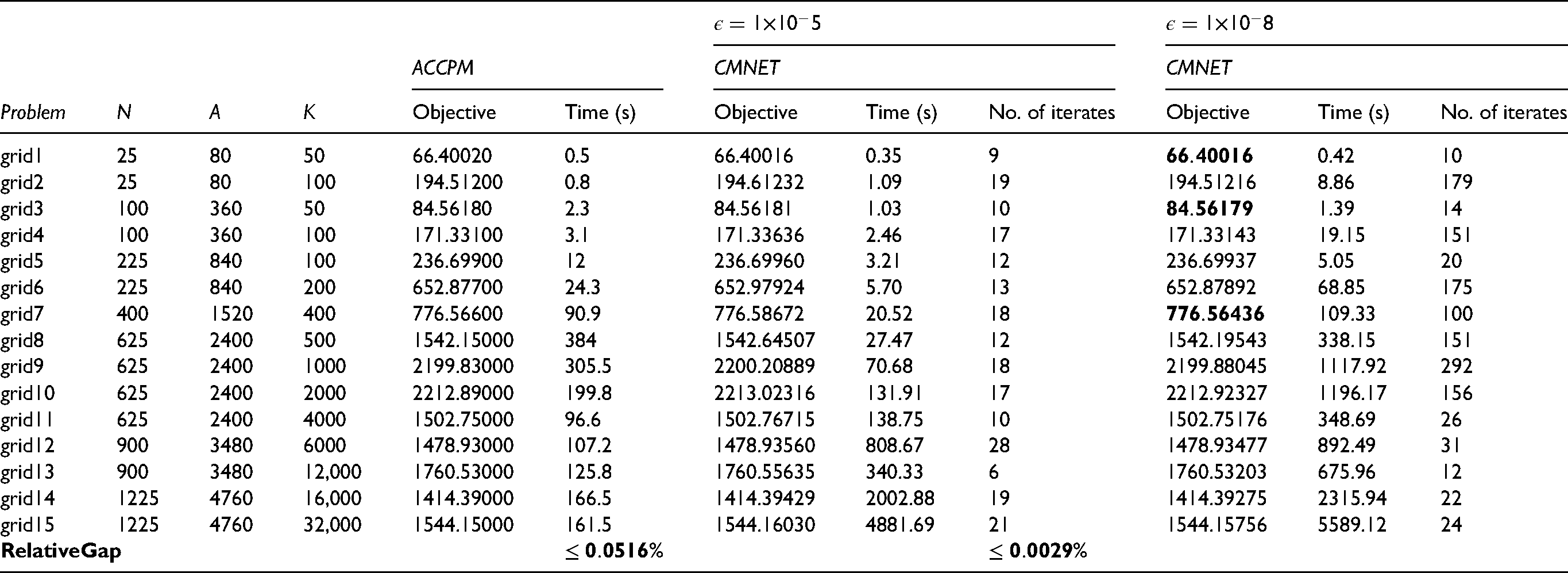
The results obtained by the CMNET on the planar and grid instances are shown in Appendices A to D. In the appendices, we also compare with the results of the ACCPM presented by Babonneau and Vial. ⁷ Since the authors did not solve planar150, we only put our solution for this instance in the tables, but do not make a comparison.

From the appendices, we see that the CMNET can solve well all test cases with separable convex costs. Even in some instances, the CMNET can obtain better solutions than those of the ACCPM such as:

Appendix A: planar30 and planar300.

Appendix B: planar80.

Appendix C: grid4, grid5, and grid9.

Appendix D: grid1, grid3, and grid7.

In the rest of these instances, the relative gap is very small. In particular, for termination condition $ϵ=1\times {10}^{-5}$ the maximum value of relative gap is 0.0516% (see Appendix D), while for $ϵ=1\times {10}^{-8}$ this value is only 0.0031% (see Appendix B).

The goal of running experiments with two termination values, $ϵ=1\times {10}^{-5}$ and $ϵ=1\times {10}^{-8}$ is to compare the computation time and the solution quality obtained by the CMNET with those of the ACCPM. The results in the column $ϵ=1\times {10}^{-5}$ from Appendices A to D show that the CMNET can find the near-optimal solutions within a reasonable computation time as compared with the ACCPM. The CMNET’s average computation time on all instances with $ϵ=1\times {10}^{-5}$ increases 2.5 times than ACCPM. With $ϵ=1\times {10}^{-5}$ , the CMNET can still find a better solution than the ACCPM (i.e. grid 1 in Appendix D). The number of better solutions found by the CMNET increases significantly when the average computation time of the CMNET increases 7.34 times than the ACCPM (see in the column $ϵ=1\times {10}^{-8}$ from Appendices A to D).

Figures 5 to 8 describe intuitively the comparison results between the CMNET and the ACCPM on the separable test cases. From these figures, we can see that the computation time for larger sized instances usually increases linearly or slightly as compared with the ACCPM. The maximum relative gap drops on planar2500 or grid8.

Figure 5.

Comparison result of the CMNET and the ACCPM on planar instances (BPR function).

Figure 6.

Comparison result of the CMNET and the on planar instances (Kleinrock function).

Figure 7.

Comparison result of the CMNET and the ACCPM on grid instances (BPR function).

Figure 8.

Comparison result of the CMNET and the ACCPM on grid instances (Kleinrock function).

Test cases with non-separable convex costs

According to our best knowledge, there is no benchmark instances of non-separable convex costs in the literature although such problems are often encountered in real-life. Hence, in this section we construct the first test cases with non-separable convex costs, which are based on the planar and grid instances with a modified objective function. The objective function includes the BPR congestion function and a new term of non-separable convex cost (i.e. the junction effect at nodes in the network). We can formulate the impact of junction effect at node $j$ as follows:

$$f_{ij}(y)=\left(\frac{y_{ij}}{\sum _k{y}_{kj}}\right)\left(\frac{\sum _k{y}_{kj}}{\theta \sum _k{c}_{kj}-\sum _k{y}_{kj}}\right)$$

(13)

where $y$ is a vector of flows at arcs in the network, and $\theta$ is a capacity coefficient which is used to determine the congestion level caused by incoming flows/arcs ( $k,j$ ) to node $j$ . Here, we only consider incoming flows to node $j$ as causes to contribute the congestion at node $j$ . Hence, the impact level of an incoming flow ( $i,j$ ) to node $j$ is calculated as the product of ratio of flow ( $i,j$ ) to sum of incoming flows at node $j$ : $(\frac{y_{ij}}{\sum _k{y}_{kj}})$ and ratio of sum of incoming flows at node $j$ to the capacity of node $j$ : $(\frac{\sum _k{y}_{kj}}{\theta \sum _k{c}_{kj}-\sum _k{y}_{kj}})$ .

The modified objective function can be rewritten by

$$g_{ij}(y)=t_{ij}{y}_{ij}(1+\frac{\alpha }{\beta +1}{\left(\frac{y_{ij}}{c_{ij}}\right)}^{\beta })+{\omega }_t\left(\frac{y_{ij}}{\theta \sum _k{c}_{kj}-\sum _k{y}_{kj}}\right)$$

(14)

where ${\omega }_t$ represents the weight of junction effect function in total cost. The function of junction effect used is closely to the Kleinrock delay function. When solving separately the BPR and Kleinrock functions, we see that the objective value of BPR function is about 10 million as large as that of Kleinrock function. Hence, we set ${\omega }_t$ = 10 million when solving the test cases of non-separable convex costs.

We illustrate the impact of non-separable cost term on total cost with planar1000 and grid15. We observe the impact when changing the capacity coefficient $\theta$ with values 0.5, 0.6, 0.7, 0.8, 0.9, 1.0, 10.0. Here, the smaller $\theta$ is, the stronger junction effect is.

Analyze, discuss and conclude

Computational results are shown in Figures 9 to 11 for planar1000, and Figures 12 to 14 for grid15. Figures 9 and 12 demonstrate the impact of junction effect to total cost on planar1000 and grid15, respectively. When decreasing the capacity coefficient $\theta$ at junction nodes (e.g. from 1 to 0.5 with deviation 0.1), the congestion magnitude at the junction nodes increases significantly. This makes total cost raise up. Comparing with the base solution (without junction effect), total cost increases approximately 3 times at the capacity coefficient 0.5 for planar1000, and 4 times for grid15.

Figure 9.

Impact of junction effect to total cost (planar1000).

Figure 10.

Comparison of objective value and computation time on ratio (planar1000).

Figure 11.

Comparison of objective value and computation time on relative gap (planar1000).

Figure 12.

Impact of junction effect to total cost (grid15).

Figure 13.

Comparison of objective value and computation time on ratio (grid15).

Figure 14.

Comparison of objective value and computation time on relative gap (grid15).

While the cost contributed by junction effect increases strongly, the cost of BPR function only increases slightly. This shows clearly when we compare the cost at capacity coefficient 0.5 and 10.

Strong impact of junction effect to total cost also affects to the complexity of non-separable network flow problems, that is, computation time to find the optimal solution. For planar1000, as considering the junction effect, the average of computation time increases 1.95 times. Especially, at the strict capacity coefficient (e.g. 0.6) the average of computation time increases up to 3.48 times as compared with the computation time of seeking the base solution. A similar trend also occurs to grid15.

While total cost increases linearly with respect to decreasing the capacity coefficient at junctions nodes, the computation time fluctuates. However, in general the computation time increases when decreasing the capacity coefficient at junctions nodes.

We also solved all instances of planar and grid for test cases with non-separable convex costs by the CMNET. The results are shown in Tables 1 and 2, respectively. Only for planar2500 with $\theta$ = 0.5, the CMNET cannot solve because of limited memory. Most all instances need more computation time to search for the optimal solution when the term of non-separable cost is integrated. The ratio of computation time between the non-separable cost instances and the separable cost instance (i.e. reference solution) is provided in Tables 3 and 4 for planar and grid instances, respectively. We see that the average computation time of the CMNET increases 3 and 16 times for planar and grid instances, respectively. This demonstrates the efficiency of the CMNET for solving the test cases with non-separable convex costs.

Table 1.

Results of the CMNET on planar instances with non-separable cost.

		${\omega }_t$ = 10 millions							${\omega }_t$ = 0
$Problem$	$CMNET$	$\theta$
		$0.5$	$0.6$	$0.7$	$0.8$	$0.9$	$1$	$10$
planar30	Objective	$2.190750\times {10}^8$	$1.761541\times {10}^8$	$1.508551\times {10}^8$	$1.342751\times {10}^8$	$1.224911\times {10}^8$	$1.137653\times {10}^8$	$5.200142\times {10}^7$	$4.445474\times {10}^7$
	Time (s)	1.19	1.23	0.63	0.46	0.38	0.38	0.38	0.52
	No. of iterations	10	11	6	4	3	3	3	7
planar50	Objective	$9.525005\times {10}^8$	$5.762907\times {10}^8$	$4.539112\times {10}^8$	$3.866600\times {10}^8$	$3.432433\times {10}^8$	$3.126639\times {10}^8$	$1.377090\times {10}^8$	$1.212368\times {10}^8$
	Time (s)	85.42	6.36	4.82	2.52	3.00	3.62	2.42	1.94
	No. of iterations	263	22	16	8	10	12	8	9
planar80	Objective	$1.586457\times {10}^9$	$1.086824\times {10}^9$	$8.572356\times {10}^8$	$7.232352\times {10}^8$	$6.360912\times {10}^8$	$5.744556\times {10}^{8}8$	$2.178872\times {10}^8$	$1.819062\times {10}^8$
	Time (s)	25.62	12.09	9.22	11.23	7.39	8.74	8.63	5.52
	No. of iterations	38	17	13	16	10	12	11	9
planar100	Objective	$1.465782\times {10}^9$	$1.066978\times {10}^9$	$8.689936\times {10}^8$	$7.505782\times {10}^8$	$6.712621\times {10}^8$	$6.140928\times {10}^8$	$2.682617\times {10}^8$	$2.291143\times {10}^8$
	Time (s)	19.19	20.08	15.80	15.24	13.04	11.03	12.32	7.14
	No. Iterations	14	15	12	12	10	8	8	6
planar150	Objective	$7.855872\times {10}^9$	$3.797494\times {10}^9$	$2.713782\times {10}^9$	$2.180323\times {10}^9$	$1.861127\times {10}^9$	$1.646278\times {10}^9$	$6.105529\times {10}^8$	$5.279887\times {10}^8$
	Time (s)	1,580.69	229.62	76.02	55.07	49.83	56.08	50.82	33.26
	No. of iterations	381	68	21	15	14	16	14	11
planar300	Objective	$2.302135\times {10}^9$	$1.950056\times {10}^9$	$1.737585\times {10}^9$	$1.593123\times {10}^9$	$1.488024\times {10}^9$	$1.407407\times {10}^9$	$7.709480\times {10}^8$	$6.907479\times {10}^8$
	Time (s)	200.67	122.72	108.84	66.47	73.52	65.38	87.70	52.96
	No. of iterations	20	12	11	7	8	7	9	7
planar500	Objective	$1.468117\times {10}^9$	$1.312565\times {10}^9$	$1.206013\times {10}^9$	$1.127716\times {10}^9$	$1.067252\times {10}^9$	$1.018313\times {10}^9$	$5.569095\times {10}^8$	$4.833101\times {10}^8$
	Time (s)	130.10	78.94	62.21	45.32	45.13	44.82	26.25	27.15
	No. of iterations	7	4	3	2	2	2	1	2
planar800	Objective	$3.142523\times {10}^9$	$2.817143\times {10}^9$	$2.594417\times {10}^9$	$2.430800\times {10}^9$	$2.304926\times {10}^9$	$2.204266\times {10}^9$	$1.298706\times {10}^9$	$1.169546\times {10}^9$
	Time (s)	348.39	243.91	176.55	172.03	178.85	105.92	105.82	80.56
	No. of iterations	4	3	2	2	2	1	1	1
planar1000	Objective	$1.021800\times {10}^{10}$	$8.690936v$	$7.786128\times {10}^9$	$7.176674\times {10}^9$	$6.732759\times {10}^9$	$6.389558\times {10}^9$	$3.729196\times {10}^9$	$3.418617\times {10}^9$
	Time (s)	2,006.47	3,196.44	1,888.65	1,296.14	2,233.48	1,049.99	874.06	918.78
	No. of iterations	15	26	15	10	17	8	6	8
planar2500	Objective	-	$2.947262\times {10}^{10}$	$2.642591\times {10}^{10}$	$2.436787\times {10}^{10}$	$2.287121\times {10}^{10}$	$2.172797\times {10}^{10}$	$1.327839\times {10}^{10}$	$1.238293\times {10}^{10}$
	Time (s)	-	36,256.03	18,444.81	17,349.80	16,306.18	17,179.85	11,326.20	11666.50
	No. of iterations	-	25	12	12	11	12	7	8

Table 2.

Results of the CMNET on grid instances with non-separable cost.

		${\omega }_t=10$ millions
$\mathrm{Problem}$	$\mathrm{CMNET}$	$\theta$
		$0.5$	$0.6$	$0.7$	$0.8$	$0.9$	$1$	$10$	${\omega }_t=0$
grid1	Objective	$3.111906\times {10}^{10}$	$9.243753\times {10}^9$	$4.225905\times {10}^8$	$2.785320\times {10}^8$	$2.142544\times {10}^8$	$1.750493\times {10}^8$	$1.078009\times {10}^7$	$8.335999\times {10}^5$
	Time (s)	0.96	0.29	0.54	0.82	0.55	0.66	0.22	0.44
	No. of iterations	13	3	7	13	8	10	2	9
grid2	Objective	$5.016990\times {10}^{11}$	$1.286580\times {10}^{11}$	$2.769531\times {10}^9$	$8.739776\times {10}^8$	$5.451362\times {10}^8$	$3.971996\times {10}^8$	$1.676195\times {10}^7$	$1.726902\times {10}^6$
	Time (s)	83.70	90.68	96.62	1.57	1.15	1.39	0.78	0.42
	No. Iterations	1000	1000	1000	19	14	17	9	6
grid3	Objective	$5.393188\times {10}^8$	$4.020119\times {10}^8$	$3.201661\times {10}^8$	$2.659610\times {10}^8$	$2.274094\times {10}^8$	$1.985624\times {10}^8$	$1.685141\times {10}^7$	$1.532418\times {10}^6$
	Time (s)	7.11	5.69	4.57	5.30	4.09	5.16	1.12	1.10
	No. of iterations	20	18	13	16	10	16	3	5
grid4	Objective	$1.266980\times {10}^9$	$8.581656\times {10}^8$	$6.482507\times {10}^8$	$5.204340\times {10}^8$	$4.344326\times {10}^8$	$3.726059\times {10}^8$	$2.854590\times {10}^7$	$3.055429\times {10}^6$
	Time (s)	22.18	16.41	10.91	8.25	6.37	6.46	1.51	2.06
	No. Iterations	60	43	28	20	14	15	3	12
grid5	Objective	$1.548514\times {10}^9$	$1.140409\times {10}^9$	$9.024649\times {10}^8$	$7.465786\times {10}^8$	$6.364964\times {10}^8$	$5.546081\times {10}^8$	$4.726632\times {10}^7$	$5.079207\times {10}^6$
	Time (s)	28.24	28.28	21.61	32.57	36.68	31.84	4.87	2.41
	No. of iterations	18	18	14	22	26	24	3	8
grid6	Objective	$7.826886\times {10}^9$	$3.959311\times {10}^9$	$2.662175\times {10}^9$	$2.007523\times {10}^9$	$1.611947\times {10}^9$	$1.346873v$	$9.162650\times {10}^7$	$1.050754\times {10}^7$
	Time (s)	239.38	145.51	92.05	44.88	29.95	29.51	12.98	5.66
	No. of iterations	175	109	68	28	18	18	8	12
grid7	Objective	$7.003848\times {10}^9$	$4.484321\times {10}^9$	$3.302495\times {10}^9$	$2.615316\times {10}^9$	$2.165788\times {10}^9$	$1.848751\times {10}^9$	$1.498749\times {10}^8$	$2.606693\times {10}^7$
	Time (s)	533.08	362.09	273.72	218.24	157.68	89.16	26.85	12.53
	No. of iterations	131	87	64	46	31	17	5	10
grid8	Objective	$1.673972\times {10}^{1}0$	$9.478416\times {10}^9$	$6.624531\times {10}^9$	$5.097262\times {10}^9$	$4.145145\times {10}^9$	$3.494353\times {10}^9$	$2.621074\times {10}^8$	$4.212406\times {10}^7$
	Time (s)	1,600.67	992.10	973.30	669.70	471.43	308.22	89.34	30.45
	No. of iterations	161	90	96	64	43	26	7	13
grid9	Objective	$4.595436\times {10}^{1}0$	$1.668445\times {10}^{1}0$	$1.024978\times {10}^{1}0$	$7.413728\times {10}^9$	$5.815285\times {10}^9$	$4.789839\times {10}^9$	$3.542035\times {10}^8$	$8.363939\times {10}^7$
	Time (s)	6,926.42	2,165.51	1,292.86	380.92	994.69	792.99	134.55	90.04
	No. of iterations	575	193	107	27	90	69	10	22
grid10	Objective	$5.966468\times {10}^{1}0$	$1.700617\times {10}^{1}0$	$1.045019\times {10}^{1}0$	$7.568890\times {10}^9$	$5.948836\times {10}^9$	$4.910370\times {10}^9$	$4.394879\times {10}^8$	$1.660848\times {10}^8$
	Time (s)	20,987.94	3,205.92	1,643.35	672.76	434.58	1,120.36	229.43	144.54
	No. of iterations	1000	229	105	36	25	78	14	19
grid11	Objective	$1.660000\times {10}^{1}0$	$9.660999\times {10}^9$	$6.873306\times {10}^9$	$5.369133\times {10}^9$	$4.428305\times {10}^9$	$3.783809\times {10}^9$	$5.575892\times {10}^8$	$3.324756\times {10}^8$
	Time (s)	4,449.69	1,932.74	761.69	1,347.42	996.43	726.01	204.58	194.711
	No. of iterations	219	89	32	64	47	33	9	14
grid12	Objective	$1.242131\times {10}^{1}0$	$8.616448\times {10}^9$	$6.663868\times {10}^9$	$5.475804\times {10}^9$	$4.676188\times {10}^9$	$4.101014\times {10}^9$	$8.369617\times {10}^8$	$5.814886\times {10}^8$
	Time (s)	3,788.06	1,309.06	1,983.94	1,184.71	778.52	769.88	251.86	237.027
	No. Iterations	81	27	43	25	16	16	5	8
grid13	Objective	$1.699347\times {10}^{1}0$	$1.127847\times {10}^{1}0$	$8.598296\times {10}^9$	$7.043901\times {10}^9$	$6.028342\times {10}^9$	$5.312461\times {10}^9$	$1.456647\times {10}^9$	$1.169337\times {10}^9$
	Time (s)	8,284.60	6,518.27	3,524.50	1,936.57	1,344.97	2,151.53	521.99	622.848
	No. of iterations	111	92	48	26	18	30	7	9
grid14	Objective	$1.150807\times {10}^{1}0$	$8.928208\times {10}^9$	$7.435499\times {10}^9$	$6.461531\times {10}^9$	$5.775457\times {10}^9$	$5.265827\times {10}^9$	$2.083582\times {10}^9$	$1.812975\times {10}^9$
	Time (s)	5,124.82	5,333.12	3,116.24	2,417.35	1,886.12	2,568.77	684.19	629.411
	No. of iterations	37	40	23	18	14	20	5	5
grid15	Objective	$1.457560\times {10}^{1}0$	$1.154448\times {10}^{1}0$	$9.832353\times {10}^9$	$8.730471\times {10}^9$	$7.961010\times {10}^9$	$7.392795\times {10}^9$	$3.904739\times {10}^9$	$3.615686\times {10}^9$
	Time (s)	7,928.48	6,542.36	6,221.99	4,855.01	4,208.44	3,130.27	1,354.24	1376.404
	No. of iterations	33	28	27	21	19	14	6	6

Table 3.

Impact of non-separable cost to the computation time of the CMNET on planar instances.

	${\omega }_t$ = 10 millions
	$\theta$
$\mathrm{Problem}$	$0.5$	$0.6$	$0.7$	$0.8$	$0.9$	$1$	$10$	$\mathrm{Average}\mathrm{ratio}$
planar30	2.27	2.36	1.21	0.89	0.73	0.72	0.72	1.27
planar50	44.03	3.28	2.48	1.30	1.55	1.87	1.24	7.96
planar80	4.64	2.19	1.67	2.04	1.34	1.58	1.56	2.15
planar100	2.69	2.81	2.21	2.13	1.83	1.55	1.72	2.13
planar150	47.52	6.90	2.29	1.66	1.50	1.69	1.53	9.01
planar300	3.79	2.32	2.06	1.26	1.39	1.23	1.66	1.96
planar500	4.79	2.91	2.29	1.67	1.66	1.65	0.97	2.28
planar800	4.32	3.03	2.19	2.14	2.22	1.31	1.31	2.36
planar1000	2.18	3.48	2.06	1.41	2.43	1.14	0.95	1.95
planar2500	-	3.11	1.58	1.49	1.40	1.47	0.97	1.67

Table 4.

Impact of non-separable cost to the computation time of the CMNET on grid instances.

	${\omega }_t$ = 10 millions
	$\theta$
$\mathrm{Problem}$	$0.5$	$0.6$	$0.7$	$0.8$	$0.9$	$1$	$10$	$\mathrm{Average}\mathrm{ratio}$
grid1	2.18	0.66	1.23	1.87	1.26	1.50	0.49	1.31
grid2	200.23	216.94	231.15	3.75	2.76	3.33	1.86	94.29
grid3	6.46	5.17	4.15	4.81	3.71	4.69	1.02	4.29
grid4	10.77	7.97	5.30	4.01	3.09	3.14	0.73	5.00
grid5	11.72	11.74	8.97	13.52	15.22	13.22	2.02	10.92
grid6	42.28	25.70	16.26	7.93	5.29	5.21	2.29	14.99
grid7	42.53	28.89	21.84	17.41	12.58	7.11	2.14	18.93
grid8	52.57	32.58	31.96	21.99	15.48	10.12	2.93	23.95
grid9	76.93	24.05	14.36	4.23	11.05	8.81	1.49	20.13
grid10	145.20	22.18	11.37	4.65	3.01	7.75	1.59	27.96
grid11	22.85	9.93	3.91	6.92	5.12	3.73	1.05	7.64
grid12	15.98	5.52	8.37	5.00	3.28	3.25	1.06	6.07
grid13	13.30	10.47	5.66	3.11	2.16	3.45	0.84	5.57
grid14	8.14	8.47	4.95	3.84	3.00	4.08	1.09	4.80
grid15	5.76	4.75	4.52	3.53	3.06	2.27	0.98	3.55

Test cases with side constraints

As mentioned in section ‘Two-phase gradient projection algorithm’, the CMNET can also solve non-separable convex multicommodity flow problems with side constraints. However, the CMNET need to be modified slightly in the process of determining feasible solution after each iteration. A Pseudo code of the modified two-phase gradient projection algorithm for non-separable convex multicommodity flow problems with side constraints is shown in Algorithm 2. We illustrate one iteration of this algorithm in Figure 15.

Algorithm 2.

$\mathbf{S}\mathbf{t}\mathbf{e}\mathbf{p}\mathbf{0.}$	$\mathbf{I}\mathbf{n}\mathbf{i}\mathbf{t}\mathbf{i}\mathbf{a}\mathbf{l}\mathbf{i}\mathbf{z}\mathbf{a}\mathbf{t}\mathbf{i}\mathbf{o}\mathbf{n}:$
	Set $h:=0$ , $ϵ:=1\times {10}^{-}8$ , and ${\beta }_0:=1000$ .
$\mathbf{S}\mathbf{t}\mathbf{e}\mathbf{p}\mathbf{1.}$	$\mathbf{S}\mathbf{h}\mathbf{o}\mathbf{r}\mathbf{t}\mathbf{e}\mathbf{s}\mathbf{t}\mathbf{p}\mathbf{a}\mathbf{t}\mathbf{h}\mathbf{a}\mathbf{n}\mathbf{d}\mathbf{G}\mathbf{S}\mathbf{S}:$
	Solve a sequence of SP and GSS with 50 times to find $x_h$ .
$\mathbf{S}\mathbf{t}\mathbf{e}\mathbf{p}\mathbf{2.}$	$\mathbf{C}\mathbf{h}\mathbf{e}\mathbf{c}\mathbf{k}\mathbf{t}\mathbf{h}\mathbf{e}\mathbf{f}\mathbf{e}\mathbf{a}\mathbf{s}\mathbf{i}\mathbf{b}\mathbf{l}\mathbf{e}\mathbf{c}\mathbf{o}\mathbf{n}\mathbf{d}\mathbf{i}\mathbf{t}\mathbf{i}\mathbf{o}\mathbf{n}:$
	$\mathbf{I}\mathbf{f}$ ( $x_h\notin {\mathbf{X}}_S$ ) where ${\mathbf{X}}_S$ is the feasible solution set including side constraints, $\mathbf{T}\mathbf{h}\mathbf{e}\mathbf{n}$ solve once $\mathbf{S}\mathbf{O}\mathbf{C}\mathbf{P}$ with $z_{h+1}:=x_h$ to obtain the feasible solution $x_{h+1}$ ;
	$\mathbf{E}\mathbf{l}\mathbf{s}\mathbf{e}$ set $x_{h+1}:=x_h$ , let $h:=h+1$ , and go to Step 3.
$\mathbf{S}\mathbf{t}\mathbf{e}\mathbf{p}\mathbf{3.}$	$\mathbf{M}\mathbf{o}\mathbf{d}\mathbf{i}\mathbf{f}\mathbf{i}\mathbf{e}\mathbf{d}\mathbf{g}\mathbf{r}\mathbf{a}\mathbf{d}\mathbf{i}\mathbf{e}\mathbf{n}\mathbf{t}\mathbf{p}\mathbf{r}\mathbf{o}\mathbf{j}\mathbf{e}\mathbf{c}\mathbf{t}\mathbf{i}\mathbf{o}\mathbf{n}:$
	Solve the $\mathbf{S}\mathbf{O}\mathbf{C}\mathbf{P}$ with $z_{h+1}:=x_h-{\beta }_h\mathrm{\nabla }g(x){|}_{x=x_h}$ .
	$\mathbf{I}\mathbf{f}$ satisfying one of the following conditions:
	$g(x_{h+1}^{SOCP})<g(x_h)$ or $\mathrm{\nabla }g{(x)}^{\prime }{|}_{x=x_{h+1}^{SOCP}}(x_h-x_{h+1}^{SOCP})<0$ ,
	$\mathbf{T}\mathbf{h}\mathbf{e}\mathbf{n}$ go to Step 4;
	$\mathbf{E}\mathbf{l}\mathbf{s}\mathbf{e}$ reduce $\beta$ a half, and go back Step 3.
$\mathbf{S}\mathbf{t}\mathbf{e}\mathbf{p}\mathbf{4.}$	$\mathbf{C}\mathbf{h}\mathbf{e}\mathbf{c}\mathbf{k}\mathbf{t}\mathbf{e}\mathbf{r}\mathbf{m}\mathbf{i}\mathbf{n}\mathbf{a}\mathbf{t}\mathbf{i}\mathbf{o}\mathbf{n}\mathbf{c}\mathbf{o}\mathbf{n}\mathbf{d}\mathbf{i}\mathbf{t}\mathbf{i}\mathbf{o}\mathbf{n}:$
	$\mathbf{I}\mathbf{f}$ satisfying the termination criterion (4),
	$\mathbf{T}\mathbf{h}\mathbf{e}\mathbf{n}$ stop and conclude that $x_{h+1}^{SOCP}:=\arg {\min }_{x\in \mathbf{X}}g(x).$
	$\mathbf{I}\mathbf{f}$ $\mathrm{\nabla }g{(x)}^{\prime }{|}_{x=x_{h+1}^{SOCP}}(x_h-x_{h+1}^{SOCP})<0$ ,
	$\mathbf{T}\mathbf{h}\mathbf{e}\mathbf{n}$ implement GSS to find an improved solution $x_{h+1}^{GSS}$ between $x_h$ and $x_{h+1}^{SOCP}$ .
	Let $h:=h+1$ , and go back Step 1.

Figure 15.

Illustration of one iteration in the two-phase gradient projection algorithm for the problem with side constraints.

To evaluate the performance of the CMNET for solving such problems, we constructed test cases with the same objective function in Section ‘Test cases with non-separable convex costs’. However, we modified a number of side constraints into the instances which are simply defined as capacity constraints at some arcs for some certain commodities. We solved planar1000 and grid12 to illustrate the capability of the CMNET for solving such problems. Here, the percentage of number of commodity which is assigned to be side constraints is 1%, 2%, and 3% of $\mathbf{K}$ , while the percentage of number of corresponding arcs is 1%, 2%, 3%, 4%, and 5% of $\mathbf{A}$ .

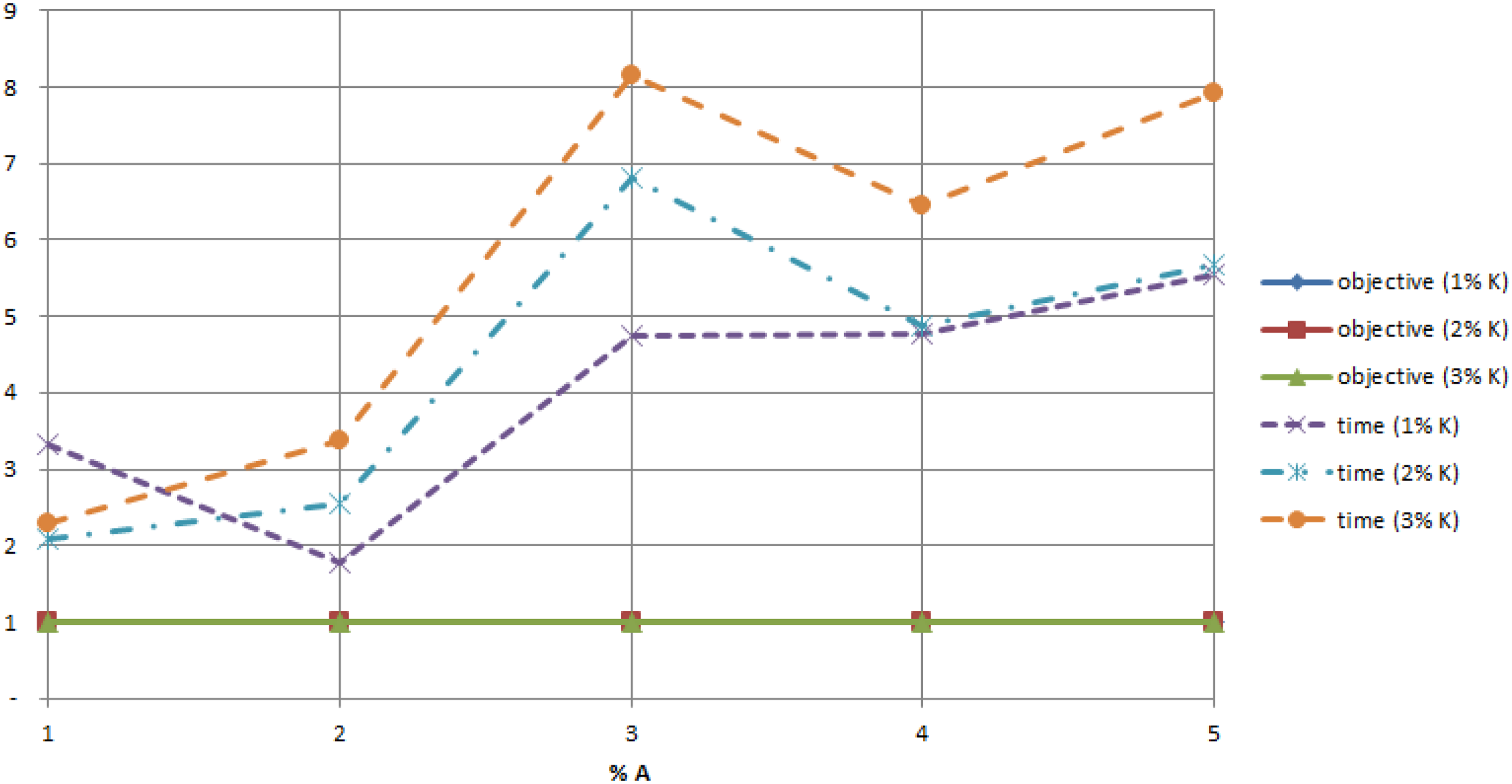
The results of the CMNET for solving planar1000 and grid12 with different number of side constraints are shown in Figures 16, 17 and 18, 19, respectively. In Figures 16 and 17, we compare the objective values and computation time of test cases with side constraints with those of separable test cases and non-separable test cases, respectively. From the results, we can see that the objective values of test cases with side constraints is not as much different as those of non-separable test cases. However, the computation time increases significantly as compared with non-separable test cases. There is the same trend of computation time for separable test cases.

Figure 16.

Comparison of solutions in separable test cases and side constraints test cases on planar1000.

Figure 17.

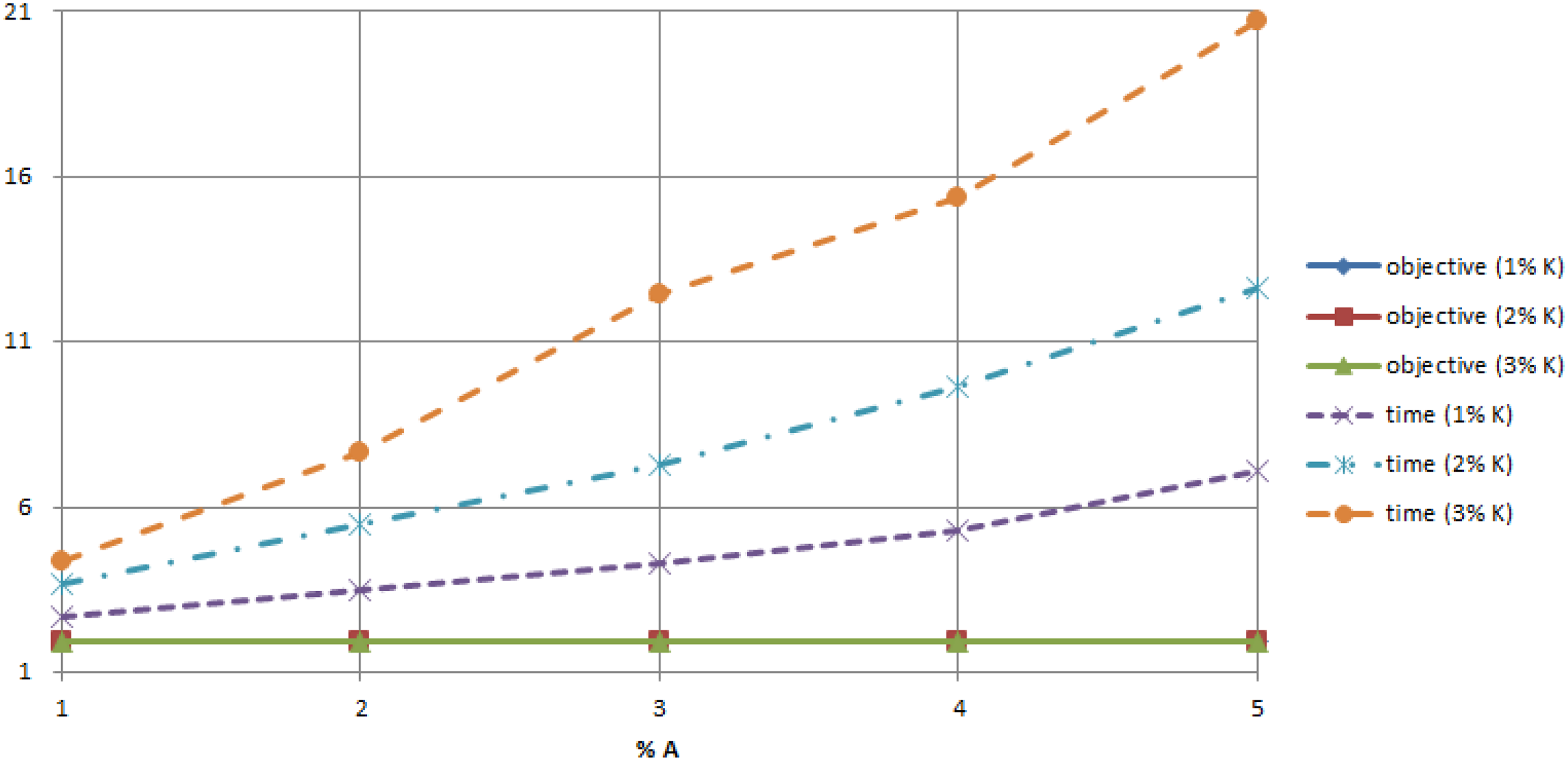
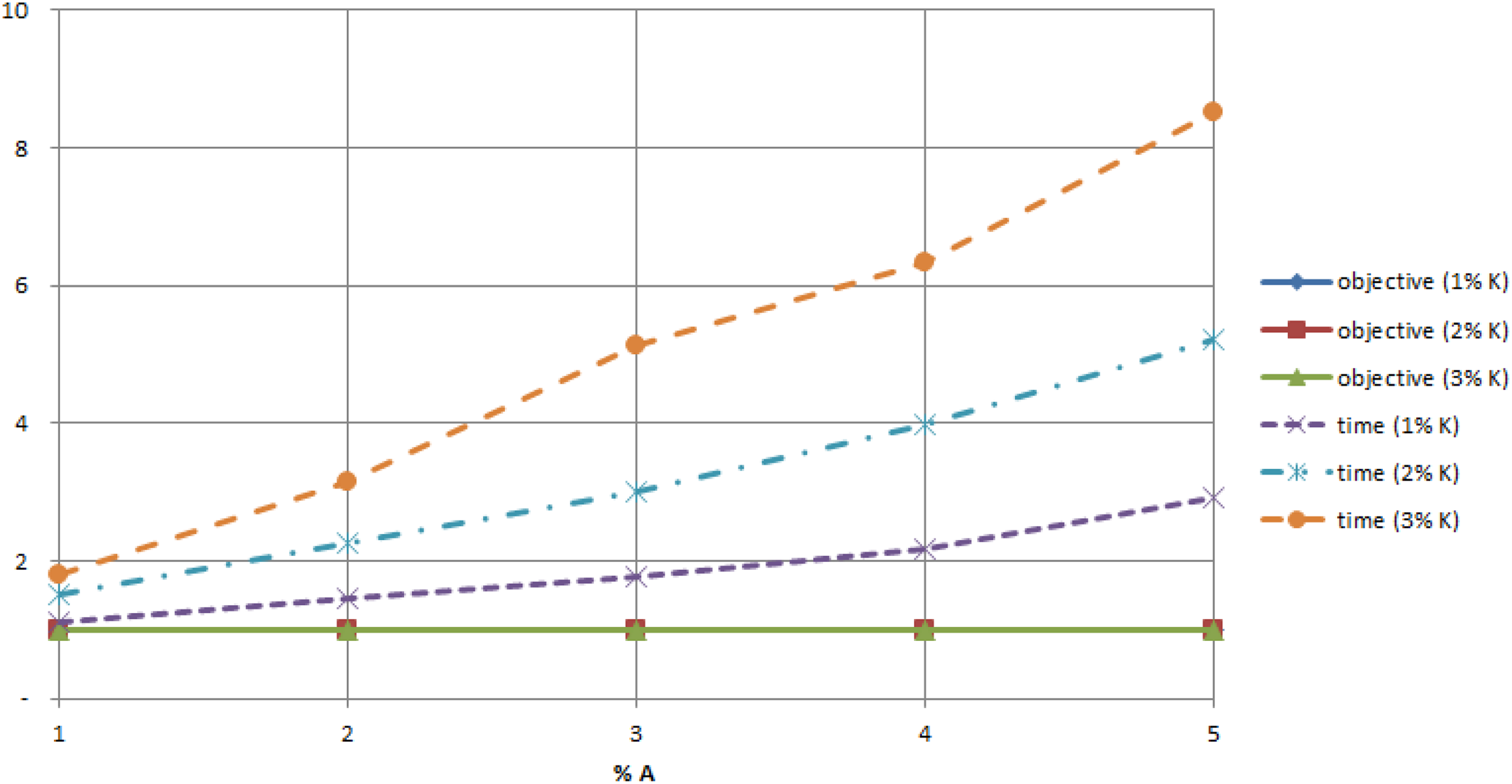
Comparison of solutions in non-separable test cases and side constraints test cases on planar1000.

Figure 18.

Comparison of solutions in separable test cases and side constraints test cases on grid12.

Figure 19.

Comparison of solutions in non-separable test cases and side constraints test cases on grid12.

We also obtain the similar results when applying the CMNET to solve grid12 with side constraints. However, the computation time for this instance increases more significantly than that of solving planar1000. This may be since the structure of grid instances is more difficult than planar instances. In general, the CMNET can handle successfully the non-separable convex network flow problems with side constraints in an increment of reasonable computation time.

In summary, while separable convex optimization is not much harder than linear optimization, ¹⁰ nonseparable optimization problems have been shown to be considerably more difficult than separable problems. ¹¹ This shows more clearly through the experiments carried out in this section. Hence, with solving successfully the non-separable convex network flow problems with side constraints the CMNET could be a promising toolbox for handling large-scale industrial applications.

Conclusions and future work

In this article, we introduce a CMNET toolbox based on a two-phase gradient projection algorithm for solving large-scale non-separable nonlinear multicommodity flow problems. The CMNET toolbox can solve multicommodity flow problems with non-separable convex costs, while other current algorithms cannot do. Also, the CMNET is applicable for practical problems where objective function not available analytically as polynomial but are evaluated using black-boxes. In addition, it can handle the problems in which additional side constraints are not of network flow types. As compared with the ACCPM on the test cases with separable convex costs, the experimental results show that the CMNET can find the optimal solutions within a reasonable increasing computation time. For the test cases with non-separable convex costs, while the ACCMP fails, the CMNET can solve them successfully. This demonstrates the promising potential of the CMNET for industrial applications where non-separable convex costs are often encountered. A possible future work is to develop this algorithm for solving the network flow problems under uncertainties or disruptions.