Adaptive time-stepping algorithms for the scalar auxiliary variable scheme of Navier-Stokes equations

Abstract

Adaptive time stepping is an important tool for controlling the simulation error and enhancing its efficiency in computational fluid dynamics. In this paper, we introduce two adaptive time-stepping algorithms based on the scalar auxiliary variable scheme for the Navier-Stokes equation. One way is to take equidistribution of energy decay to control the variance of the time steps, and in the other way, the relative error is involved to produce time steps. The numerical experiments show that the computational time is significantly saved by these methods.

Introduction

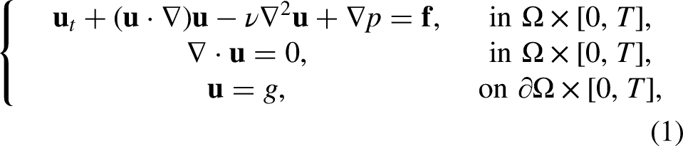
We consider an incompressible flow contained in some domain $\mathrm{\Omega }$ in two dimensions, whose boundary is denoted by $\mathrm{\partial }\mathrm{\Omega }$ . The dynamics of the flow is described by the incompressible Navier-Stokes equations, given in a non-dimensional form as follows

$$\{\begin{array}{ccc}& {\mathbf{u}}_t+(\mathbf{u}\cdot \mathrm{\nabla })\mathbf{u}-\nu {\mathrm{\nabla }}^2\mathbf{u}+\mathrm{\nabla }p=\mathbf{f},& \text{in}\mathrm{\Omega }\times [0,T]\\ & \mathrm{\nabla }\cdot \mathbf{u}=0,& \text{in}\mathrm{\Omega }\times [0,T]\\ & \mathbf{u}=g,& \text{on}\mathrm{\partial }\mathrm{\Omega }\times [0,T]\end{array}$$

(1)

where $u:\mathrm{\Omega }\times [0,T]\to {\mathbb{R}}^2$ is the fluid velocity, black $\mathbf{g}:\mathrm{\partial }\mathrm{\Omega }\times [0,T]\to {\mathbb{R}}^2$ is the boundary velocity and $p:\mathrm{\Omega }\times [0,T]\to \mathbb{R}$ is the fluid pressure. The body force $\mathbf{f}$ is known, and $\nu$ is the kinematic viscosity of the fluid. The system is supplemented by the initial condition

$$\mathbf{u}(\mathbf{x},0)={\mathbf{u}}_0(\mathbf{x})$$

(2)

and the following often-used condition to fix the pressure values

$${\int }_{\mathrm{\Omega }}p=0$$

(3)

There have been extensive works for the Navier-Stokes equations. Semi-implicit splitting type schemes de-couple the computations for the velocity and the pressure fields and enjoy the constant coefficient matrices, but they are only conditionally stable (see Guermond et al. ¹ and the references therein). To alleviate the time step size constraint, unconditionally energy-stable schemes are preferred, but involve the solution of a system of non-linear algebraic equations or a system of linear algebraic equations with a variable and time-dependent coefficient matrix (see e.g. Labovsky et al. ² and Sanderse ³ ). Recently, by introducing a scalar auxiliary energy variable the authors in ⁴ reformulated the incompressible Navier-Stokes equations (1) to (3) into an equivalent gradient-flow system including a linear constant coefficient system and a nonlinear algebraic equation. However, the cost by solving the above nonlinear equation is negligible since it is about a scalar number, not a field function. Numerical experiments show that the computational cost of this algorithm per time step is approximately twice that of the semi-implicit scheme, but the above auxiliary energy is proven to be unconditionally stable in, ⁴ which allows time steps based on the accuracy requirement only.

In many gradient-flow systems, energy evolution may undergo large and small variations at different time intervals. By enjoying the unconditionally energy stability, the scalar auxiliary variable (SAV) methods can be easily combined with an adaptive strategy. Hence, small time steps are only used when the energy variation is large, while larger time steps can be used when the energy variation is small (see e.g. Cheng and Shen ⁵ ). Unlike applying variable time steps to first-order schemes without affecting the unconditional stability, we shall construct a new SAV scheme by modifying the scheme in, ⁴ in order to preserve unconditional stability for second-order schemes with variable time steps.

The above adaptive time-stepping technique was developed based on the energy derivative in time in ⁶ and also used in ⁷ for the Cahn-Hilliard problem. In Xu and Tang, ⁸ based on the stabilisation method there, one can use a large time step in the computation. The spectral deferred correction methods were proposed in ⁹ and applied in ¹⁰ to solve the phase field problems. Recently, adaptive time-stepping methods based on the energy were proposed in,^11,12 but only first-order accurate in time. Hence, we shall propose the first adaptive SAV time-stepping algorithm for the above reformulated Navier-Stokes problem (see Algorithm 1), which are based on the auxiliary energy and second-order accurate in time.

Methods to produce time steps in simulations by other ways is also widely considered. The authors in ⁵ presented a multiple SAV (MSAV) scheme for the phase field equations, which are extremely efficient when coupled with adaptive time-stepping. Similarly based on the relative errors for the first- and second-order schemes, the second adaptive time stepping algorithm will be presented to shorten the simulation time (see Algorithm 2). Finally, we shall use the numerical examples to illustrate the algorithms.

SAV algorithm and some properties

Reformulated system and semi-discrete schemes

First, we recall the following equivalent formulation to (1) introduced by Lin et al., ⁴ which is based on the SAV approach:

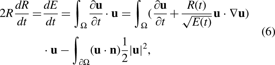
Introduce the total blackkinetic energy as

$$E(t)=C_0+{\int }_{\mathrm{\Omega }}\frac{1}{2}|\mathbf{u}{|}^{2}d\mathbf{x}$$

(4)

where we choose $C_0$ to be a constant such that $E(t)>0$ for all $t\ge 0$ . Then we define

$$R(t)=\sqrt{E(t)}$$

(5)

We derive that from the divergence free condition

$$\begin{array}{rl}2R\frac{dR}{dt}=& \frac{dE}{dt}={\int }_{\mathrm{\Omega }}\frac{\mathrm{\partial }\mathbf{u}}{\mathrm{\partial }t}\cdot \mathbf{u}={\int }_{\mathrm{\Omega }}(\frac{\mathrm{\partial }\mathbf{u}}{\mathrm{\partial }t}+\frac{R(t)}{\sqrt{E(t)}}\mathbf{u}\cdot \mathrm{\nabla }\mathbf{u})\\ & \cdot \mathbf{u}-{\int }_{\mathrm{\partial }\mathrm{\Omega }}(\mathbf{u}\cdot \mathbf{n})\frac{1}{2}|\mathbf{u}{|}^2\end{array}$$

(6)

where $\mathbf{n}$ denotes the unit normal vector on $\mathrm{\partial }\mathrm{\Omega }$ .

Therefore, the Navier-Stokes equations (1) can be rewritten into an equivalent form

$$\{\begin{array}{cc}& \frac{\mathrm{\partial }\mathbf{u}}{\mathrm{\partial }t}+\frac{R(t)}{\sqrt{E(t)}}(\mathbf{u}\cdot \mathrm{\nabla })\mathbf{u}-\nu {\mathrm{\nabla }}^2\mathbf{u}+\mathrm{\nabla }p=\mathbf{f}\\ & \mathrm{\nabla }\cdot \mathbf{u}=0\\ & 2R\frac{dR}{dt}={\displaystyle {\int }_{\mathrm{\Omega }}(\frac{\mathrm{\partial }\mathbf{u}}{\mathrm{\partial }t}+\frac{R(t)}{\sqrt{E(t)}}\mathbf{u}\cdot \mathrm{\nabla }\mathbf{u})\cdot \mathbf{u}-{\displaystyle {\int }_{\mathrm{\partial }\mathrm{\Omega }}(\mathbf{u}\cdot \mathbf{n})\frac{1}{2}|\mathbf{u}{|}^2}}\end{array}$$

(7)

Thus, to approximate this reformulated equivalent system of equations (7), we present the following first- and second-order schemes for variant time steps by modifying the schemes in ⁴ for constant time steps.

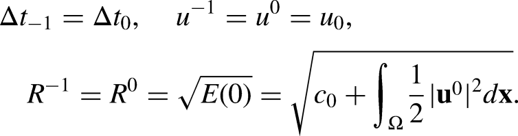
• Let $\{t_n\}$ be an increasing sequence with $t_0=0$ , and set $\mathrm{\Delta }{t}_n=t_{n+1}-t_n$ . We set the ghost and initial condition as

  $$\mathrm{\Delta }{t}_{-1}=\mathrm{\Delta }{t}_0,u^{-1}=u^0=u_0,R^{-1}=R^0=\sqrt{E(0)}=\sqrt{c_0+{\int }_{\mathrm{\Omega }}\frac{1}{2}|{\mathbf{u}}^0{|}^{2}d\mathbf{x}}$$

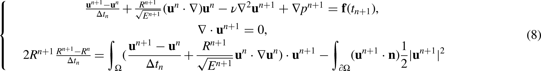
• Then given $({\mathbf{u}}^{n-1},R^{n-1})$ and $({\mathbf{u}}^n,p^n,R^n)$ , we can compute $({\mathbf{u}}^{n+1},p^{n+1},R^{n+1})$ through the first-order scheme:

  $$\{\begin{array}{ccc}& \frac{{\mathbf{u}}^{n+1}-{\mathbf{u}}^n}{\mathrm{\Delta }{t}_n}+\frac{R^{n+1}}{\sqrt{E^{n+1}}}({\mathbf{u}}^n\cdot \mathrm{\nabla }){\mathbf{u}}^n-\nu {\mathrm{\nabla }}^2{\mathbf{u}}^{n+1}+\mathrm{\nabla }{p}^{n+1}=\mathbf{f}(t_{n+1})& \\ & \mathrm{\nabla }\cdot {\mathbf{u}}^{n+1}=0& \\ & 2R^{n+1}\frac{R^{n+1}-R^n}{\mathrm{\Delta }{t}_n}={\displaystyle {\int }_{\mathrm{\Omega }}(\frac{{\mathbf{u}}^{n+1}-{\mathbf{u}}^n}{\mathrm{\Delta }{t}_n}+\frac{R^{n+1}}{\sqrt{E^{n+1}}}{\mathbf{u}}^n\cdot \mathrm{\nabla }{\mathbf{u}}^n)\cdot {\mathbf{u}}^{n+1}-{\displaystyle {\int }_{\mathrm{\partial }\mathrm{\Omega }}({\mathbf{u}}^{n+1}\cdot \mathbf{n})\frac{1}{2}|{\mathbf{u}}^{n+1}{|}^2}}& \end{array}$$

  (8)
  or the second-order scheme:
  $$\{\begin{array}{ccc}& \frac{{\gamma }_1{\mathbf{u}}^{n+1}-{\gamma }_2{\mathbf{u}}^n+{\gamma }_3{\mathbf{u}}^{n-1}}{\mathrm{\Delta }{t}_n+\mathrm{\Delta }{t}_{n-1}}+\frac{R^{n+1}}{\sqrt{E^{n+1}}}({\overline{\mathbf{u}}}^n\cdot \mathrm{\nabla }){\overline{\mathbf{u}}}^n-\nu {\mathrm{\nabla }}^2{\mathbf{u}}^{n+1}+\mathrm{\nabla }{p}^{n+1}=\mathbf{f}(t_{n+1})& \\ & \mathrm{\nabla }\cdot {\mathbf{u}}^{n+1}=0& \\ & 2R^{n+1}\frac{{\gamma }_1{R}^{n+1}-{\gamma }_2{R}^n+{\gamma }_3{R}^{n-1}}{\mathrm{\Delta }{t}_n+\mathrm{\Delta }{t}_{n-1}}={\displaystyle {\int }_{\mathrm{\Omega }}(\frac{{\gamma }_1{\mathbf{u}}^{n+1}-{\gamma }_2{\mathbf{u}}^n+{\gamma }_3{\mathbf{u}}^{n-1}}{\mathrm{\Delta }{t}_n+\mathrm{\Delta }{t}_{n-1}}+\frac{R^{n+1}}{\sqrt{E^{n+1}}}{\overline{\mathbf{u}}}^n\cdot \mathrm{\nabla }{\overline{\mathbf{u}}}^n)\cdot {\mathbf{u}}^{n+1}-{\displaystyle {\int }_{\mathrm{\partial }\mathrm{\Omega }}({\mathbf{u}}^{n+1}\cdot \mathbf{n})\frac{1}{2}|{\mathbf{u}}^{n+1}{|}^2}}& \end{array}$$

  (9)
  with
  $${\overline{\mathbf{u}}}^n=\frac{\mathrm{\Delta }{t}_n+\mathrm{\Delta }{t}_{n-1}}{\mathrm{\Delta }{t}_{n-1}}{\mathbf{u}}^n-\frac{\mathrm{\Delta }{t}_n}{\mathrm{\Delta }{t}_{n-1}}{\mathbf{u}}^{n-1}$$

  (10)
  and
  $${\gamma }_1=\frac{2\mathrm{\Delta }{t}_n+\mathrm{\Delta }{t}_{n-1}}{\mathrm{\Delta }{t}_n},{\gamma }_2=\frac{(\mathrm{\Delta }{t}_n+\mathrm{\Delta }{t}_{n-1}{)}^2}{\mathrm{\Delta }{t}_n\mathrm{\Delta }{t}_{n-1}},{\gamma }_3=\frac{\mathrm{\Delta }{t}_n}{\mathrm{\Delta }{t}_{n-1}}$$

  (11)
  with the boundary condition to be ${\mathbf{u}}^{n+1}=\mathbf{g}(t_{n+1})$ on $\mathrm{\partial }\mathrm{\Omega }$ .

Remark 0.1

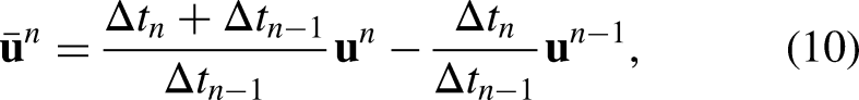
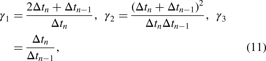
If $v$ denotes a generic variable, then in the above equations $\frac{{\gamma }_1{v}^{n+1}-{\gamma }_2{v}^n+{\gamma }_3{v}^{n-1}}{\mathrm{\Delta }{t}_n+\mathrm{\Delta }{t}_{n-1}}$ is the second order approximation of ${\mathrm{\partial }}_{t}v(t_{n+1})$ with ${\gamma }_i,i=1,2,3$ defined specifically by (11). Furthermore, ${\overline{\mathbf{u}}}^n$ defined by (10) denotes a second-order explicit approximation of $\mathbf{u}(t_{n+1})$ .

Remark 0.2

If each time step is a constant, that is, $\mathrm{\Delta }{t}_{n-1}=\mathrm{\Delta }{t}_n=\mathrm{\Delta }t$ , we have

$$\frac{{\gamma }_1{v}^{n+1}-{\gamma }_2{v}^n+{\gamma }_3{v}^{n-1}}{\mathrm{\Delta }{t}_n+\mathrm{\Delta }{t}_{n-1}}=\frac{3v^{n+1}-4v^n+v^{n-1}}{2\mathrm{\Delta }{t}_n},{\overline{\mathbf{u}}}^n=2{\mathbf{u}}^n-{\mathbf{u}}^{n-1}$$

Thus the schemes (8) and (9) go back to the corresponding ones in. ⁴

The main advantage for the above schemes (8) and (9) lies in that they both enjoy the following unconditional energy stability. In the subsequent analysis, we let $(u,v)$ and $<u,v>$ denote the $L^2$ inner product of $u,v$ in the domain $\mathrm{\Omega }$ and $\mathrm{\partial }\mathrm{\Omega }$ , respectively, and the norm $\Vert v\Vert =\sqrt{(v,v)}$ .

Lemma 0.1

⁴ Theorem 2.1 In the absence of the external force $\mathbf{f}$ and with zero boundary velocity $\mathbf{g}$ , the first-order scheme (8) satisfies the following property:

$$Q^{n+1}-Q^n=-\Vert D^{n+1}{\Vert }^2-\nu \mathrm{\Delta }t\Vert \mathrm{\nabla }{\mathbf{u}}^{n+1}{\Vert }^2$$

(12)

where

$$Q^n=|R^n{|}^2,D^{n+1}=R^{n+1}-R^n$$

(13)

The proof for the first-order scheme (8) was blackprovided by Lin et al. ⁴ Theorem 2.1, thus we only give a proof for the second-order scheme (9) as follows.

Lemma 0.2

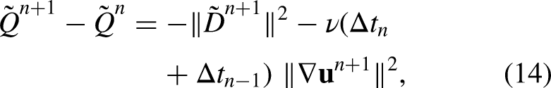
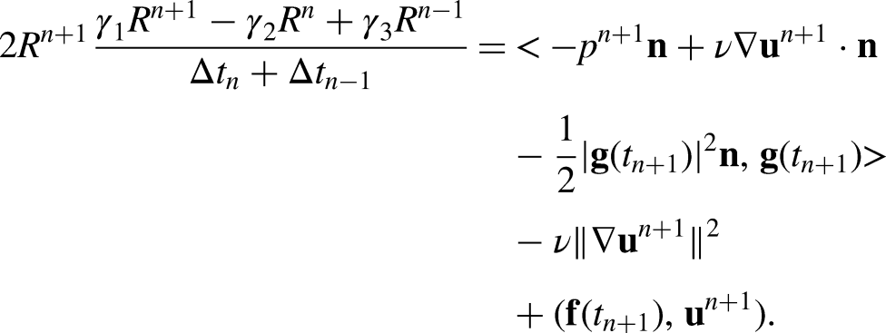
In the absence of the external force $\mathbf{f}$ and with zero boundary velocity $\mathbf{g}$ , the second scheme (9) to (11) satisfies the following property:

$${\tilde{Q}}^{n+1}-{\tilde{Q}}^n=-\Vert {\tilde{D}}^{n+1}{\Vert }^2-\nu (\mathrm{\Delta }{t}_n+\mathrm{\Delta }{t}_{n-1})\Vert \mathrm{\nabla }{\mathbf{u}}^{n+1}{\Vert }^2$$

(14)

where

$$\begin{array}{c}{\tilde{Q}}^n={\left|\frac{\sqrt{{\gamma }_2}-\sqrt{{\gamma }_2-4{\gamma }_3}}{2}{R}^n\right|}^2+{|\sqrt{{\gamma }_2}{R}^n-\frac{\sqrt{{\gamma }_2}-\sqrt{{\gamma }_2-4{\gamma }_3}}{2}{R}^{n-1}|}^2\\ {\tilde{D}}^{n+1}=\frac{2{\gamma }_3}{\sqrt{{\gamma }_2}-\sqrt{{\gamma }_2-4{\gamma }_3}}{R}^{n+1}-\sqrt{{\gamma }_2}{R}^n+\frac{\sqrt{{\gamma }_2}-\sqrt{{\gamma }_2-4{\gamma }_3}}{2}{R}^{n-1}\end{array}$$

(15)

Proof.

First, taking the inner product of the first equation in (11) with ${\mathbf{u}}^{n+1}$ leads to

$$\begin{array}{rl}& (\frac{{\gamma }_1{\mathbf{u}}^{n+1}-{\gamma }_2{\mathbf{u}}^n+{\gamma }_3{\mathbf{u}}^{n-1}}{\mathrm{\Delta }{t}_n+\mathrm{\Delta }{t}_{n-1}}+\frac{R^{n+1}}{\sqrt{E^{n+1}}}({\overline{\mathbf{u}}}^n\cdot \mathrm{\nabla }){\overline{\mathbf{u}}}^n,{\mathbf{u}}^{n+1})\\ & +<{\mathbf{u}}^{n+1}\cdot \mathbf{n},p^{n+1}>-\nu <\mathrm{\nabla }{\mathbf{u}}^{n+1}\cdot \mathbf{n},{\mathbf{u}}^{n+1}>\\ & +\nu \Vert \mathrm{\nabla }{\mathbf{u}}^{n+1}{\Vert }^2=(\mathbf{f}(t_{n+1}),{\mathbf{u}}^{n+1})\end{array}$$

where we used the divergence free condition. Then we sum up the above equation and the third equation in (11) to obtain

$$\begin{array}{rl}2R^{n+1}\frac{{\gamma }_1{R}^{n+1}-{\gamma }_2{R}^n+{\gamma }_3{R}^{n-1}}{\mathrm{\Delta }{t}_n+\mathrm{\Delta }{t}_{n-1}}=& <-p^{n+1}\mathbf{n}+\nu \mathrm{\nabla }{\mathbf{u}}^{n+1}\cdot \mathbf{n}\\ & -\frac{1}{2}|\mathbf{g}(t_{n+1}){|}^2\mathbf{n},\mathbf{g}(t_{n+1})>\\ & -\nu \Vert \mathrm{\nabla }{\mathbf{u}}^{n+1}{\Vert }^2\\ & +(\mathbf{f}(t_{n+1}),{\mathbf{u}}^{n+1})\end{array}$$

Finally, combined with the following relation

$$2R^{n+1}({\gamma }_1{R}^{n+1}-{\gamma }_2{R}^n+{\gamma }_3{R}^{n-1})={\tilde{Q}}^{n+1}-{\tilde{Q}}^n+\Vert {\tilde{D}}^{n+1}{\Vert }^2$$

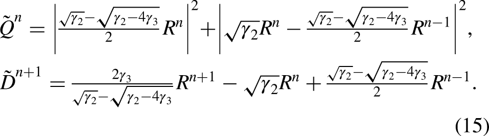
where we used the definitions (15), we obtain the desired stability result (14).  □

Solution algorithm and implementation

Even though at first glance both the schemes (8) and (9) look like coupled and implicit systems of equations, in fact they can be implemented in a very efficient way (cf. Lin et al. ⁴ ), thanks to the fact that $R^{n+1}$ and $E^{n+1}$ are scalar numbers, not field functions. We next only explain the details to implement the scheme (8), since the ones for the scheme (9) are similar.

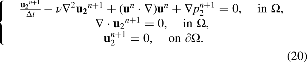
First, we introduce a auxiliary variable $S$ to separate ${\mathbf{u}}^{n+1}$ and $p^{n+1}$ as follows

$$S=\frac{R^{n+1}}{\sqrt{E^{n+1}}},{\mathbf{u}}^{n+1}={{\mathbf{u}}_{\mathbf{1}}}^{n+1}+S{{\mathbf{u}}_{\mathbf{2}}}^{n+1},p^{n+1}=p_1^{n+1}+S{p}_2^{n+1}$$

(16)

Then from (4) we can see that

$$E^{n+1}=E(S)=c_0+{\int }_{\mathrm{\Omega }}\frac{1}{2}|{\mathbf{u}}^{n+1}{|}^2=A_0+A_{1}S+A_2{S}^2$$

(17)

with

$$A_0=c_0+{\int }_{\mathrm{\Omega }}\frac{1}{2}|{\mathbf{u}}_1^{n+1}{|}^2,A_1={\int }_{\mathrm{\Omega }}{\mathbf{u}}_1^{n+1}\cdot {\mathbf{u}}_2^{n+1},A_2={\int }_{\mathrm{\Omega }}\frac{1}{2}|{\mathbf{u}}_2^{n+1}{|}^2$$

(18)

Implementation of algorithm:

• By substituting (16) into (8), we can separate (8) by two linear subproblems, from which we can solve $\{{{\mathbf{u}}_{\mathbf{i}}}^{n+1},p_i^{n+1}\},i=1,2$ , respectively

  $$\{\begin{array}{ccc}& \frac{{{\mathbf{u}}_{\mathbf{1}}}^{n+1}-{\mathbf{u}}^n}{\mathrm{\Delta }{t}_n}-\nu {\mathrm{\nabla }}^2{{\mathbf{u}}_{\mathbf{1}}}^{n+1}+\mathrm{\nabla }{p}_1^{n+1}=\mathbf{f}(t_{n+1}),\text{in}\mathrm{\Omega }& \\ & \mathrm{\nabla }\cdot {{\mathbf{u}}_1}^{n+1}=0,\text{in}\mathrm{\Omega }& \\ & {\mathbf{u}}_1^{n+1}=\mathbf{g}(t_{n+1}),\text{on}\mathrm{\partial }\mathrm{\Omega }\end{array}$$

  (19)
  and
  $$\{\begin{array}{ccc}& \frac{{{\mathbf{u}}_{\mathbf{2}}}^{n+1}}{\mathrm{\Delta }t}-\nu {\mathrm{\nabla }}^2{{\mathbf{u}}_{\mathbf{2}}}^{n+1}+({\mathbf{u}}^n\cdot \mathrm{\nabla }){\mathbf{u}}^n+\mathrm{\nabla }{p}_2^{n+1}=0,\text{in}\mathrm{\Omega }& \\ & \mathrm{\nabla }\cdot {{\mathbf{u}}_2}^{n+1}=0,\text{in}\mathrm{\Omega }& \\ & {\mathbf{u}}_2^{n+1}=0,\text{on}\mathrm{\partial }\mathrm{\Omega }\end{array}$$

  (20)

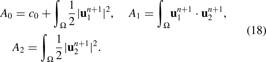
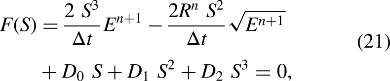
• Substituting (16) into the third equation of (8), then the unknown $S$ can be obtained by solving the following algebraic equation

  $$\begin{array}{rl}F(S)& =\frac{2S^3}{\mathrm{\Delta }t}{E}^{n+1}-\frac{2R^n{S}^2}{\mathrm{\Delta }t}\sqrt{E^{n+1}}\\ & +D_{0}S+D_1{S}^2+D_2{S}^3=0\end{array}$$

  (21)
  with
  $$\{\begin{array}{rl}& D_0=\nu \Vert \mathrm{\nabla }{\mathbf{u}}_1^{n+1}{\Vert }^2-(\mathbf{f}(t_{n+1}),{\mathbf{u}}_1^{n+1})+<p_1^{n+1}\mathbf{n}-\nu \mathbf{n}\cdot \mathrm{\nabla }{\mathbf{u}}_1^{n+1}+\frac{1}{2}|\mathbf{g}(t_{n+1}){|}^2\mathbf{n},\mathbf{g}(t_{n+1})>\\ & D_1=2\nu (\mathrm{\nabla }{\mathbf{u}}_1^{n+1},\mathrm{\nabla }{\mathbf{u}}_2^{n+1})-(\mathbf{f}(t_{n+1}),{\mathbf{u}}_2^{n+1})+<p_2^{n+1}\mathbf{n}-\nu \mathbf{n}\cdot \mathrm{\nabla }{\mathbf{u}}_2^{n+1},\mathbf{g}(t_{n+1})>& \\ & D_2=\nu \Vert \mathrm{\nabla }{\mathbf{u}}_2^{n+1}{\Vert }^2& \end{array}$$

  (22)
  Here we can use the Newton’s method to solve (21) with the initial guess $S=1$ , and the cost of the computation is very small compared to the total cost within a time step since it is a scalar nonlinear algebraic equation for $S$ .

• With $S$ known, we can compute the scalar function $E^{n+1}$ from (17) and $\{R^{n+1},{\mathbf{u}}^{n+1},p^{n+1}\}$ from (16).

Adaptive time-stepping algorithm

We introduce two adaptive time-stepping methods in this section. First, we shall show how to produce the adaptive time step. Then we proposed the adaptive time-stepping algorithms.

An adaptive time step: based on energy: We first use the energy decay to control the variance of the time steps. A transform of discrete energy identities (12) and (14) are $\mathrm{\Delta }{t}_n=-\frac{Q^{n+1}-Q^n+\Vert D^{n+1}{\Vert }^2}{\nu \Vert \mathrm{\nabla }{\mathbf{u}}^{n+1}{\Vert }^2}$ and $\mathrm{\Delta }{t}_n=-\frac{{\tilde{Q}}^{n+1}-{\tilde{Q}}^n+\Vert {\tilde{D}}^{n+1}{\Vert }^2}{\nu \Vert \mathrm{\nabla }{\mathbf{u}}^{n+1}{\Vert }^2}-\mathrm{\Delta }{t}_{n-1}$ for the first- and second-order schemes, respectively. As we aim at equidistribution of the energy decay, we allow the numerator $|Q^{n+1}-Q^n+\Vert D^{n+1}{\Vert }^2|$ or $|{\tilde{Q}}^{n+1}-{\tilde{Q}}^n+\Vert {\tilde{D}}^{n+1}{\Vert }^2|$ to be a constant $\delta E$ . Thus the time step turns to $\mathrm{\Delta }{t}_n=\frac{\delta E}{\nu \Vert \mathrm{\nabla }{\mathbf{u}}^{n+1}{\Vert }^2}$ or $\mathrm{\Delta }{t}_n=\frac{\delta E}{\nu \Vert \mathrm{\nabla }{\mathbf{u}}^{n+1}{\Vert }^2}-\mathrm{\Delta }{t}_{n-1}$ . But we find there is still an unknown term ${\mathbf{u}}^{n+1}$ in the denominator. We therefore replace ${\mathbf{u}}^{n+1}$ by ${\mathbf{u}}^n$ (or ${\overline{\mathbf{u}}}^n$ defined by (10)) for the first- (or second-) order scheme to get a computable adaptive time step

$$\mathrm{\Delta }{t}_n=\frac{\delta E}{\nu \Vert \mathrm{\nabla }{\mathbf{u}}^n{\Vert }^2},\text{or}\mathrm{\Delta }{t}_n=\frac{\delta E}{\nu \Vert \mathrm{\nabla }{\overline{\mathbf{u}}}^n{\Vert }^2}-\mathrm{\Delta }{t}_{n-1}$$

(23)

An adaptive time step: based on error: Given the solutions at $t_{n-1}$ and $t_n$ , we compute $({\mathbf{u}}_f,p_f,R_f{)}^{n+1}$ by the first-order scheme (8) and $({\mathbf{u}}_s,p_s,R_s{)}^{n+1}$ by the second-order schemes (9), respectively. Then we can use the following relative error

$$e_{n+1}=max\{\frac{\Vert {\mathbf{u}}_s^{n+1}-{\mathbf{u}}_f^{n+1}\Vert }{\Vert {\mathbf{u}}_s^{n+1}\Vert },\frac{\Vert p_f^{n+1}-p_s^{n+1}\Vert }{\Vert p_s^{n+1}\Vert }\}$$

(24)

as the indicator to control the time step. One simple but effective strategy is to update the time step size by using the formula ⁵

$$A_{dp}(e,\mathrm{\Delta }t)=\rho {\left(\frac{tol}{e}\right)}^{1/2}\mathrm{\Delta }t$$

where $e$ is a relative error, $\mathrm{\Delta }t$ is the time step, $tol$ is the error tolerance and $\rho$ is an artificial parameter.

Based on the discussion, two adaptive time stepping Algorithms 1 and 2 on equidistribution of the energy decay and the relative error are proposed as below, respectively.

Algorithm 1.

SAV adaptive time-stepping method: Based on energy

Ensure:

1. Set $\mathrm{\Delta }{t}_{min}$ and $\mathrm{\Delta }{t}_{max}$ , compute the problem (8) or (9) with the minimal time step $\mathrm{\Delta }{t}_{min}$ for some steps. Set $\delta E$ as the average of the energy decay and set $m=1$ .

2. At the time $t_n$ , compute the time step with formula (23), and then the problem (8) or (9) with time step $\mathrm{\Delta }{t}_n=min(\mathrm{\Delta }{t}_{max},max(\mathrm{\Delta }{t}_n,\mathrm{\Delta }{t}_{min}))$ .

3. Check if energy decay of two successive steps $\le \delta E$ and $\mathrm{\Delta }{t}_n=\mathrm{\Delta }{t}_{min}$ . If neither, return to Step 2 with time step $\mathrm{\Delta }{t}_n=min(\mathrm{\Delta }{t}_{max},max(\mathrm{\Delta }{t}_n/2,\mathrm{\Delta }{t}_{min}))$ .

4. If $\mathrm{\Delta }{t}_n=\mathrm{\Delta }{t}_{min}$ , adjust $\delta E$ with an arithmetic average $$\delta E=\frac{m\times \delta E+\text{energy decay}}{m+1},$$

and set $m=m+1$ .

5. Set $t_{n+1}=t_n+\mathrm{\Delta }{t}_n$ , set $n=n+1$ and go to Step 2.

Algorithm 2.

SAV adaptive time-stepping method: based on error

Ensure:

1. Set $\mathrm{\Delta }{t}_{min}$ and $\mathrm{\Delta }{t}_{max}$ , compute the problem (8) with the minimal time step $\mathrm{\Delta }{t}_{min}$ for some steps. Set $tol$ and $\rho$ .

2. At the time $t_n$ , compute $(u_f,p_f{)}^{n+1}$ by the first order scheme (8) with $\mathrm{\Delta }{t}_n$ .

3. Compute $(u_s,p_s{)}^{n+1}$ by the second order schemes (9) with $\mathrm{\Delta }{t}_{n-1}$ and $\mathrm{\Delta }{t}_n$ .

4. Calculate $e_{n+1}$ by formula (24).

5. If $e_{n+1}tol$ return to Step 2 with time step $\mathrm{\Delta }{t}_n=max(\mathrm{\Delta }{t}_{min},min(\mathrm{\Delta }{t}_{max},A_{dp}(e_{n+1},\mathrm{\Delta }{t}_n)))$ , else update time step $\mathrm{\Delta }{t}_n=max(\mathrm{\Delta }{t}_{min},min(\mathrm{\Delta }{t}_{max},A_{dp}(e_{n+1},\mathrm{\Delta }{t}_n)))$ .

6. Set $t_{n+1}=t_n+\mathrm{\Delta }{t}_n$ , set $n=n+1$ and go to Step 2.

Numerical experiments

In this section, we implement the adaptive time-stepping methods, Algorithms 1 and 2, for the Navier-Stokes equations on a single computer serially. We use the first-order Lagrange finite element (cf. Girault and Raviart ¹³ ) to approximate both the velocity and the pressure fields in the space discretization based on a sufficiently small constant mesh size. The Newton iteration method is used to solve the nonlinear algebraic equation (21). The tolerances for the Newton iteration method is set to be ${10}^{-9}$ and the artificial parameters $\mathrm{\Delta }{t}_{max}$ , $\mathrm{\Delta }{t}_{min}$ can be chosen arbitrarily.

Taylor-Green vortex

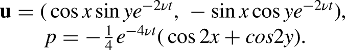
We consider the Taylor-Green vortex model (1) on a square domain $\mathrm{\Omega }=[0,\pi ]\times [0,\pi ]$ with the analytical solution as follows

$$\begin{array}{cc}& \mathbf{u}=(\cos x\sin y{e}^{-2\nu t},-\sin x\cos y{e}^{-2\nu t})\\ & p=-\frac{1}{4}{e}^{-4\nu t}(\cos 2x+cos2y)\end{array}$$

We choose the parameters $\nu =1$ and $T=1.$ Then, the terms $\mathbf{f}$ , $\mathbf{g}$ and ${\mathbf{u}}_0$ can be chosen based on the above analytical solution.

This test problem is historically used to assess accuracy, convergence rates and adaptive time stepping in CFD.^14,15 Here we also do detailed research on this problem to show the usability of our adaptive time-stepping algorithms. The numerical results are obtained on a $1500\times 1500$ grid in space. For Algorithm 1, we use the average energy decay in the time interval $[0.05,0.1]$ as $\delta E$ and for Algorithm 2, we choose the parameters $tol=1E-5$ and $\rho =\mathrm{0.6.}$

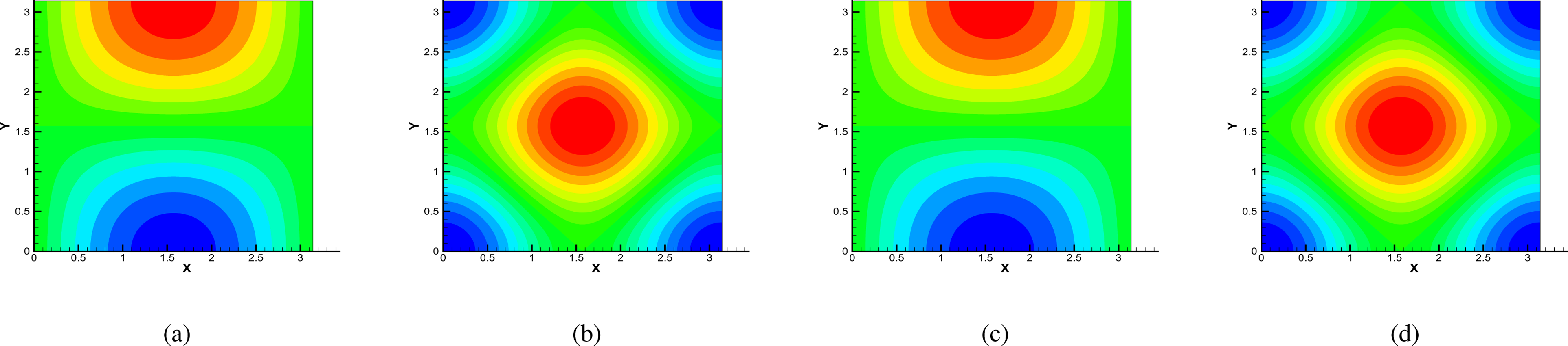
The comparison of the unknowns. Some pictures of the unknowns at the final time are shown in Figures 1 to 3. The first two ones of Figures 1 and 2 are the numerical results computed by the first-order scheme (8) and second-order schemes (9) with uniform step, respectively, and the last two are the numerical results computed by the first- and second-order schemes in Algorithm 1, respectively. Then the two ones of Figure 3 are the numerical results computed by Algorithm 2. From the pictures, we can see every unknown looks almost the same, the difference of which in $L^2$ norm is about $O({10}^{-3})$ .

Figure 1.

The contour of the Taylor-Green vortex problem using first-order scheme in Algorithm 1: (a) velocity (uniform step $\mathrm{\Delta }t=0.001$ ), (b) pressure (uniform step $\mathrm{\Delta }t=0.001$ ), (c) velocity (adaptive step $\mathrm{\Delta }{t}_{min}=0.001,\mathrm{\Delta }{t}_{max}=0.015$ ) and (d) pressure (adaptive step $\mathrm{\Delta }{t}_{min}=0.001,\mathrm{\Delta }{t}_{max}=0.015$ ).

Figure 2.

The contour of the Taylor-Green vortex problem using second-order scheme in Algorithm 1: (a) velocity (uniform step $\mathrm{\Delta }t=0.001$ ), (b) pressure (uniform step $\mathrm{\Delta }t=0.001$ ), (c) velocity (adaptive step $\mathrm{\Delta }{t}_{min}=0.001,\mathrm{\Delta }{t}_{max}=0.1$ ) and (d) pressure (adaptive step $\mathrm{\Delta }{t}_{min}=0.001,\mathrm{\Delta }{t}_{max}=0.1$ ).

Figure 3.

The contour of the Taylor-Green vortex problem using Algorithm 2: (a) velocity (adaptive step $\mathrm{\Delta }{t}_{min}=0.001,\mathrm{\Delta }{t}_{max}=0.1$ ) and (b) pressure (adaptive step $\mathrm{\Delta }{t}_{min}=0.001,\mathrm{\Delta }{t}_{max}=0.1$ ).

The evolution of the energy, relative error and the corresponding time steps. Figure 4 shows the evolution of energy and relative error as well as the corresponding time steps, which are produced by the first-order and second-order adaptive schemes, (8) and (9), of Algorithm 1, respectively, and Figure 5 are produced by Algorithm 2.

Figure 4.

The evolution in Algorithm 1: (a) energy decay, (b) the evolution of time steps and (c) CPU time.

Figure 5.

The evolution in Algorithm 2 : (a) relative error between first-order and second-order schemes, (b) the evolution of time steps and (c) CPU time.

The computational time. In Figures 4 and 5, ‘time’ labelled in the horizontal coordinate-axis represents the time variable in equation (1) and ‘CPU time’ labelled in the vertical coordinate-axis is the computation cost, from which we can find both adaptive methods do actually save computational time and only take less than one-third of the time of the uniform method.

Lid-driven cavity flow

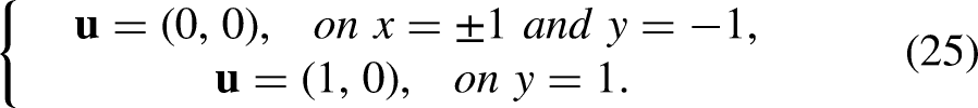
In order to show validity of the adaptive SAV method, we test lid-driven cavity flow problem. The computational domain is the unite square domain, and the boundary conditions are

$$\{\begin{array}{ccc}& \mathbf{u}=(0,0),onx=\pm 1andy=-1& \\ & \mathbf{u}=(1,0),ony=1& \end{array}$$

(25)

We choose the $\nu =1/100,\mathrm{\Delta }{t}_{min}={10}^{-6},\mathrm{\Delta }{t}_{max}=5.0\times {10}^{-3},h=1/4000$ . The streamlines and the time steps by Algorithm 1 are shown in Figure 6.

Figure 6.

The evolution in Algorithm 1: (a) streamlines and (b) the evolution of time steps.

Then we choose the $\nu =1/1000,\mathrm{\Delta }{t}_{min}={10}^{-6},\mathrm{\Delta }{t}_{max}=5.0\times {10}^{-3},h=1/4000$ . The streamlines and the time steps by Algorithm 1 are shown in Figure 7.

Figure 7.

The evolution in Algorithm 2 : (a) streamlines, (b) the evolution of time steps when $0⩽t⩽245$ and (c) the evolution of time steps when $0⩽t⩽0.06$ .

From the above figures, it can be found that at the beginning the accuracy can be guaranteed only when the time step is very small. With the development of time, the time step can be larger, which indeed saves the computation time compared with the constant time step.

Footnotes

Declaration of conflicting interests

The authors declared no potential conflicts of interest with respect to the research, authorship and/or publication of this article.

Funding

This work is in part supported by the National Natural Science Foundation of China (no. 11871410), the Natural Science Foundation of Fujian Province of China (nos. 2021J01034, 2018J01004), the Fundamental Research Funds for the Central Universities (no. 20720180001).

ORCID iD

Hongtao Chen