The normalized Laplacian spectrum of a graph is an important tool that one can use to find much information about its topological and structural characteristics and also on some relevant dynamical aspects, specifically in relation to random walks. In this paper we devise an essentially algorithm to obtain the approximating graphs of a class of general Sierpinski triangles and their normalized Laplacian spectra, and illustrate such algorithm by a quasi-program of Matlab. In the meantime, our work also enriches the graphs whose spectrum is known.
Spectral graph theory is an interesting topic, in a way, be regarded as the study of relation between graph properties and Laplacian matrix spectrum or adjacency matrix spectrum.1–4 The spectrum of a graph(the set of eigenvalues of a graph with their multiplicities) is important in the spectral graph theory, because almost all major graph invariants are related to it, such as connectivity, expanding property, isoperimetric number, maximum cut, independence number, genus, diameter, bandwidth-type parameters, etc (see2,5,6 and the reference therein).
Spectral graph theory has different applications in different scientific fields, such as the eigenvalues were related to the stability of molecules in chemistry, graph spectra occured naturally in minimizing energies of Hamiltonian systems in physics, the recent progress on expander graphs and eigenvalues was initiated by problems of communication networks in computer science, etc. In recent years, there has been a particular interest in the study of the eigenvalues and eigenvectors of normalized Laplacian matrix, since much important information about structural properties and dynamical processes of a graph or network is related to it. In the structural aspect, for example, F. R. Chung2 proved that the number of spanning trees in a network can be determined in terms of the product of all nonzero eigenvalues of a connected network. H. Chen and F. Zhang7 showed the resistance distance can be naturally expressed by the eigenvalues and eigenvectors of normalized Laplacian matrix. With respect to dynamical process, there has been great progress in determining the eigenvalues and eigenvectors of normalized Laplacian matrix, including the first-passage time,8 mixing time9 and Kemeny’s constant10 that can be used as a measure of the efficiency of navigation on the network. Particularly, normalized Laplacian eigenvalues and eigenvectors also are relevant in light harvesting,11 energy or exciton transport,12 chemical kinetics,13 and many other problems in chemical physics.14
Let
be an equilateral triangle with lower-left coordinate (0, 0) and side 1, where and . Given an integer , write
For and , we define
By,15 there is a unique non-empty compact subset K(n) of satisfying the following set equation:
We shall call K(n) a general Sierpinski triangle throughout this paper. A familiar example of a general Sierpinski triangle is the Sierpinski gasket, in which n = 2, . Recently, evolving networks are usually modeled by the general Sierpinski triangles. For example, J. Guan et al.16 and A. Le et al.17 used the classical Sierpinski triangle to construct evolving networks.
We define , and recurrently
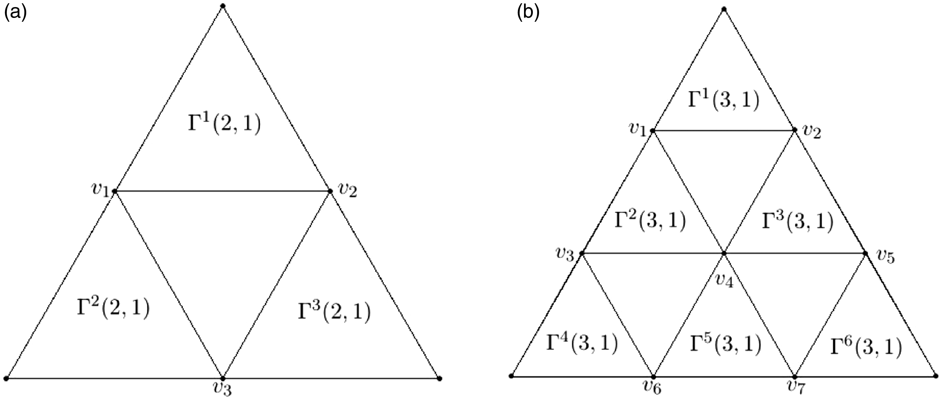
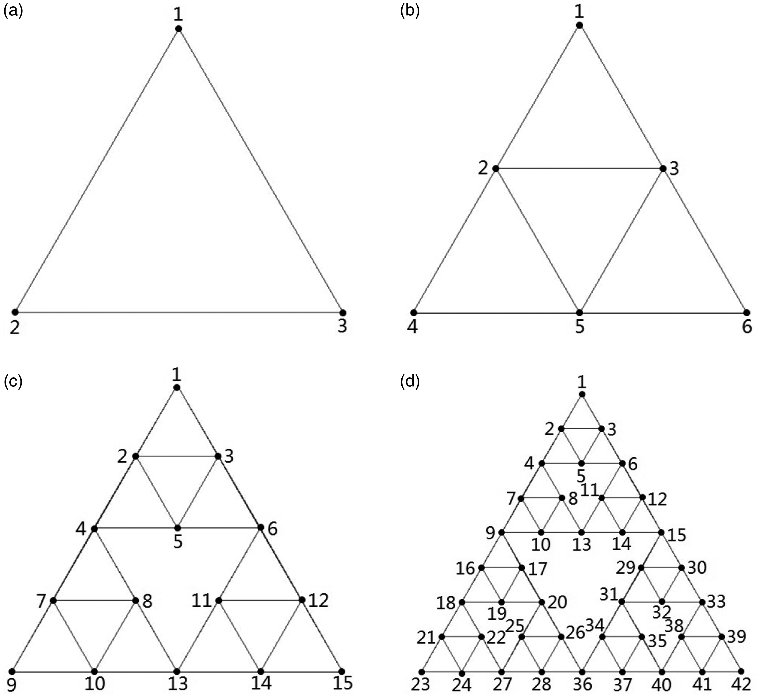
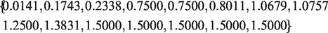
for . Then is an equilateral triangle with side 1, is a union of smaller equilateral triangles with side and converges to K(n) as in the Hausdorff metric.15 We call the k-th approximating graph of general Sierpinski triangle K(n), in which vertex set and edge set are considered in a usually way (see Figure 1 for n = 2 and k = 0, 1, 2). Another interesting motivation of our work comes form the theory of analysis on fractals. J. Kigami constructed in18 a Laplacian on the Sierpinski gasket, and later extended their method to the p.c.f. (post-critically finite) fractals. Kigami’s idea is to approximate the Laplacian on K(n) by the normalized Laplacian on . This coincide with the known graph Laplacian whose vertex set is V(n, k), where V(n, k) is described as in ‘Some basic structure properties and concepts on approximating graph’ section.
Approximation graphs of classical Sierpinski triangle , k = 0, 1, 2.
There has been notable progress on the study of the spectrum of normalized Laplacian matrix associated to fractal, especially in recent years. Yet much is still unknown, and in this direction the existed works concentrate mainly on the theoretical study base on a recursive method (or decimation method19) as we know of. For example, A.Julaiti et al. in20 studied the spectra of normalized Laplacian matrices for a family of proposed fractal trees and Cayley trees. M. Dai et al. in21 presented a study on the spectrum of the normalized Laplacian of weighted tree-like fractals. In this paper we will obtain the approximating graphs and their normalized Laplacian spectra from an algorithmic point of view, which extends the work of B. Rajan et al..22 Our method is completely different from the decimation method. Our algorithm need to code the vertices of each approximating graph base on the theory of iterated function system (IFS),15 we call it an IFS coding algorithm throughout this paper. This is of great relevance in studying the structure and some properties of general Sierpinski triangles and related graphs, and dynamical aspects of related networks in a new perspective.
This paper is organized as follows. The next section is preliminaries. We introduce the geometrical construction, normalized Laplacian matrix and some basic structure properties of approximating graph . In the subsequent section, we present our main result, called IFS coding algorithm, and illustrate our algorithm by a quasi-program of Matlab. Furthermore we also prove the correctness of this program and show the convergence of the algorithm in this section. The paper is concluded with conclusions.
Some basic structure properties and concepts on approximating graph
It is well known that a graph can be represented visually by drawing a dot for every vertex, and drawing a line segment between two vertices if they are connected by an edge. According to,23 for any , we can obtain a drawing of with as follows: We divide the equilateral triangle into n2 congruent triangles by connecting n equipartition points of each pair of edges and replace it with the union of all the upward equilateral triangles. We can now apply this process to each of these upward equilateral triangles, and then repeat the procedure to the k-th step, to obtain a drawing of with . Obviously, for any is an undirected graph without loops and multiple edges, i.e., a simple graph. Let V(n, k) and E(n, k) denote the vertex set and edge set of , respectively. For any , if u and v are connected by an edge in E(n, k), then we denote it by , and say that they are adjacent. Write
We call the adjacency matrix of . For any , we use to denote the number of edges which touch v, and call it the degree of v. Let D(n, k) denote the diagonal matrix in which the (v, v)-th entry is . We call the Laplacian matrix of . For the matrix A, let denote the inverse of A and raise each element of A to the power of half. For random walk on , the Markov matrix (or probability transition matrix) is defined as
which can be normalized to obtain the following real and symmetric matrix
We see from the definition that the (u, v)-th entry of P(n, k) is
Furthermore, M(n, k) and P(n, k) have the same spectrum since M(n, k) and P(n, k) are similar.
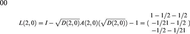
Definition 2.1. Let I be a unit matrix with the same size as P(n, k). We define the normalized Laplacian matrix of by
Example 2.1. Let n = 2 and k = 0. Then
and
are the adjacency matrix, diagonal matrix, Markov matrix, Laplacian matrix and normalized Laplacian matrix of , respectively.
Let be a simple graph with vertex set V(G) and edge set E(G), and be another simple graph. We say that G and H are isomorphic, and denote it by , if there exists a bijection such that
We say that H is a subgraph of G if and . Let denote the cardinality of a set A. For given integer , we see from the geometrical construction of that for any consists of subgraphs that are isomorphic to . We denote by these subgraphs of , respectively, see Figure 2 for n = 2, 3, and let denote the corresponding vertex sets, respectively. Note that if with , then is a singleton, which is unique common vertex of small triangles and . It easy to check that has the following obviously structure properties.
and their subgraphs . (a) n= 2 and (b) n = 3.
Proposition 2.2.For,
Proposition 2.3.Forand, let V(n, k) andbe defined as above. Then for any.
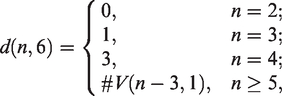
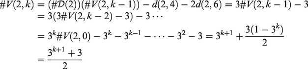
Proposition 2.4.For, let d(n, m) denote the total number of vertices with degree m in, m = 2, 4 and 6. Then
and forand.
Proposition 2.5.Letand.Then
and.
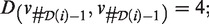
Example 2.2.Let n = 2. Thenandfor. SeeFigure 3for.
Coding of using IFS coding algorithm. (a) k = 0. (b) k = 1. (c) k = 2. (d) k = 3.
Proof. For , we have from the Propositions 2.2, 2.4 and 2.5 that
Combing the fact that , we have for . Using Proposition 2.5 again and the fact , we get that for . This proof is completed. □
Similarly, we have
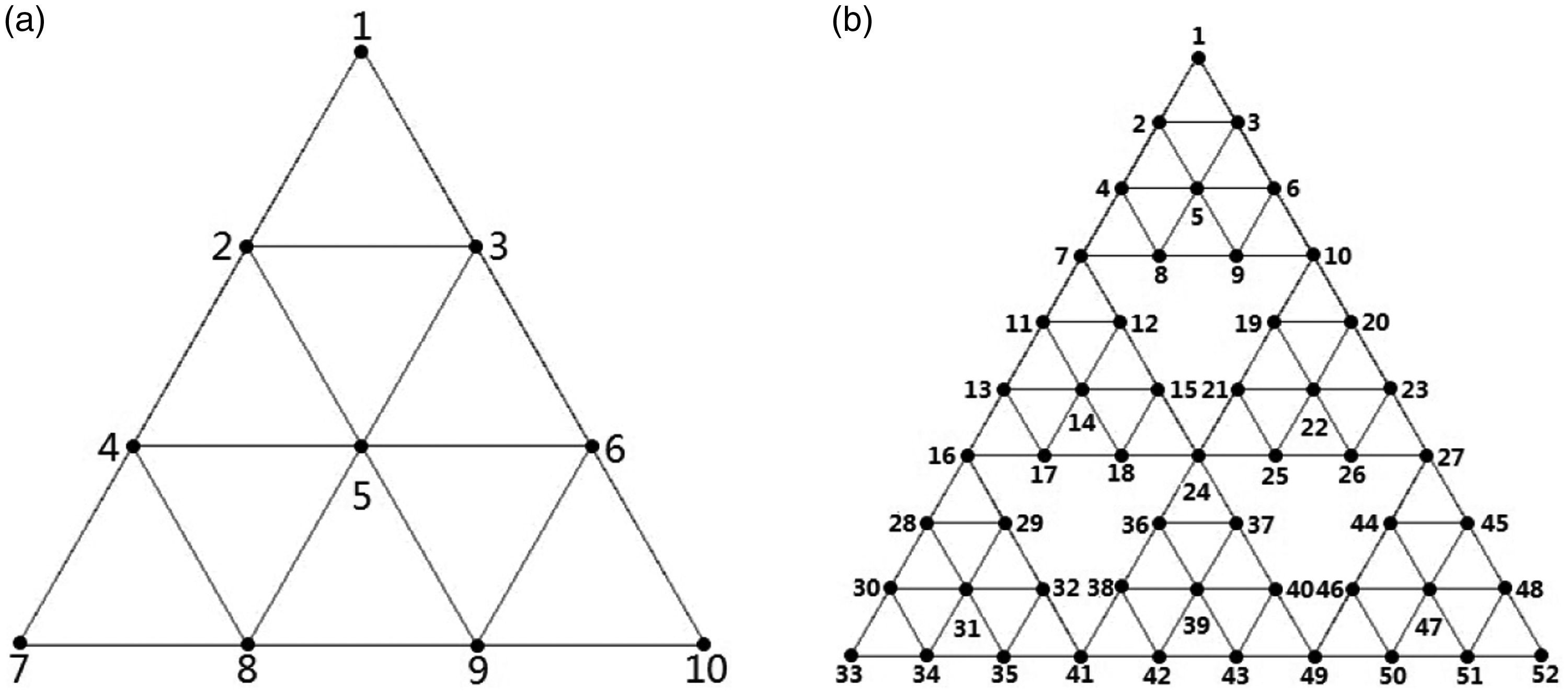
Example 2.3.Let n = 3. Then, andandfor. SeeFigure 4for.
Coding of using IFS coding algorithm. (a) k = 1. (b) k = 2.
IFS coding algorithm and a quasi-program of Matlab
Our aim in this paper is to describe completely the normalized Laplacian spectrum of for any . In view of Definition 2.1, we first need to find the adjacency matrix A(n, k) and the diagonal matrix D(n, k) of , which is the most important and most central part. However writing down manually the adjacency matrix and diagonal matrix is unimaginable when n and k are large enough. So we in this section devise an algorithm base on the iterative generation process of , called IFS coding algorithm, to code the vertices of , and thus from the adjacency matrix (resp. the diagonal matrix ) find the adjacency matrix A(n, k) (resp. the diagonal matrix D(n, k)) by the recursive relation between (resp. ) and A(n, k) (resp. D(n, k)).
Let , be described as in ‘Some basic structure properties and concepts on approximating graph’ section. Denote
Step 1: Code the vertices of as shown in Figure 3(a).
Step 2: For any , code the vertices of as that in . By Proposition 2.5, the code of v2 in is . We define and . Note that the uncoded vertices of induce a graph isomorphic to for , the uncoded vertices of induce a graph isomorphic to for , and the uncoded vertices of induce a graph isomorphic to for . Combing Propositions 2.4 and 2.5, for each vertex j in , we code the corresponding vertex of by
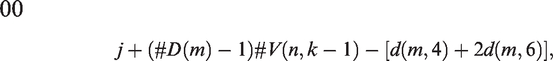
where For each vertex j in , we code the corresponding vertex of by
where . For each vertex j in , we code the corresponding vertex of by j+(i−1) V(n,k−1)−[d(n−1,4)+2d(n−1,6)]−[2(i−D(n−1))−1], where . We refer to Figure 3 for n = 2 and k = 1, 2, 3, and Figure 4 for n = 3 and k = 1, 2.
Step 3: Input the diagonal matrix and adjacency matrix of .
Step 4: Output the diagonal matrix and adjacency matrix of in term of coding rule of Step 2.
Step 5: Compute the normalized Laplacian matrix of by (2.1) and output eigenvalues.
For simplify, we write
where . In the following we illustrate our algorithm by a quasi-program of Matlab, which one need to normalize it according to Matlab syntax rules before using it, see Example 3.2. We denote by the percent-sign % an explanation.
A quasi-program of Matlab base on the IFS coding algorithm
Function Sierpinskispectrum(n,m) %is side length of each small triangle inand m is iterated depth.
% A and D are the adjacency matrix and diagonal matrix of, respectively.
% Output the adjacency matrix and diagonal matrix of.
If m = 1
A; D;
else
for
Adjmatrix(i, A); ;
end
end
% Output the eigenvalues of normalized Laplacian matrix of. spectrum )
Function Adjmatrix(k, A)
% Determine the codes ofwhich are described as in (1).
for
end
for
for
end
end
for
end
for
end
% Output the adjacency matrix of.
for
for
blkdiag;
end
blkdiag;
end
for
end
for
for ;
if k = 2
else
end
end
end
for
end
for % We define.if k = 2
else
end
end
Function Diagmatrix(k, A) % Output the diagonal matrix of.
% Using the same process as that of Function Adjmatrix(k, A), we can determine the codes of, we omit details.
for
for
blkdiag;
end
blkdiag;
end
for
end
for
for ;
end
end
for
end
for
end
Using the induction on iterated depth m for given integer , we can give the proof of correctness of above program as follows.
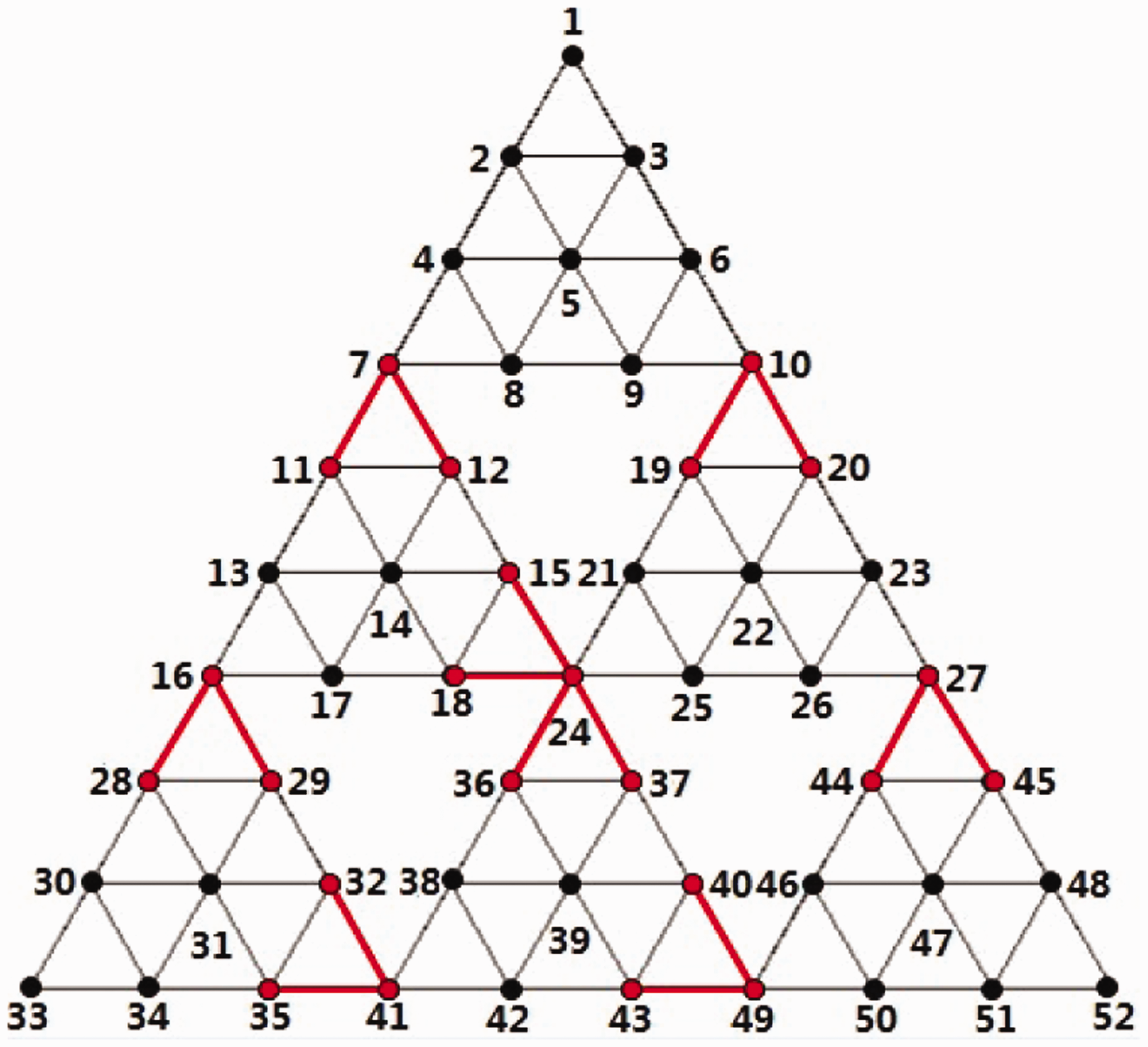
Proof of correctness of program: Without loss of generality, we show that the program is correct for the adjacency matrix. It is easy to see that this is true when m = 1, 2. Assume it is true for the case m – 1 with . Consider the case m. Let A be the adjacency matrix of . Then the adjacency matrix of is A since is isomorphic to . By Step 2, the uncoded vertices of induce a graph isomorphic to for , the uncoded vertices of induce a graph isomorphic to for , and the uncoded vertices of induce a graph isomorphic to for . We can get that the adjacency matrix Ai of by deleting the first row and column of A for , and the adjacency matrix Ai of by deleting the first row and column and the last row and column of A for . Using the function ‘blkdiag’ of Matlab, we obtain a matrix with the form
where the elements are denoted by to be accounted for as follows(such as Example 3.1). The elements in are due to all the edges except edges (see 16 red edges shown in Figure 5 for n = 3). The elements corresponding to these edges in are assigned 1 by the statements below the statement “blkdiag” in function Adjmatrix(k, A) and the others in are 0. This completes this proof.
16 missing edges for n = 3 and k = 2.
Example 3.1.Let n = 2 and m = 1. From Example 2.1, we see that
is the adjacency matrix of . Then the matrix (2) is
which is the adjacency matrix of .
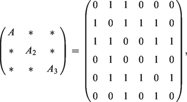
Example 3.2. See Figure 6, a Matlab program for n = 2. Input Sirpinskispectrum(3), we can obtain the adjacency matrix, diagonal matrix, normalized Laplacian matrix (see Figure 7), and the spectrum of normalized Laplacian matrix of :
A Matlab program for n = 2.
The adjacency matrix, diagonal matrix and normalized Laplacian matrix of using Matlab. (a) The adjacency matrix A. (b) The diagonal matrix D. (c) The normalized Laplacian matrix L.
Recall that V(n, k) and denote the vertex set and the normalized Laplacian matrix of the approximating graph with , respectively. Fix . It is well known that for any , the normalized Laplacian matrix can be viewed as an operator (called it normalized Laplacian) on the space of functions , see.2 Let denote the normalized Laplacian corresponding to .
We remark that our algorithm is convergent. In fact, is dense in K(n) in the natural topology18 and we have from the [24, Section ‘From graphs to fractals’] that there exists a normalized Laplacian on K(n) such that
where whose restriction on V(n, k) is . This implies our algorithm is convergent.
Conclusion
We have developed an approach to compute the normalized Laplacian spectra of approximating graphs of a class of general Sierpinski triangles in this paper. It’s easy to see that we can also get the spectra of adjacency matrix, Laplacian matrix, Markov matrix, normalized Markov matrix and signless Laplacian matrix 6 using same method. Our approach could be also used to obtain the similar approximating graphs associated with some fractals generated by iterated function system and their various spectra, such as, when one replace the Δ in this paper by a regular tetrahedron in . Future work should include studying the various topological properties of these approximating graphs like connectedness, toughness, etc; determining the spectra of networks associated with general Sierpinski triangle, and measuring the related structural properties and dynamical processes, specifically in relation to random walk.
Footnotes
Acknowledgements
The author would like to thank the referees for carefully reading the paper and making several helpful suggestions which led to the improvement of the manuscript. Part of this work was carried out when the author was visiting the Department of Mathematical Sciences of Georgia Southern University. He thanks the Department for its hospitality and support during his visit. The author would also like to thank Liuna Dang, Xiaojiu LU Fu Yalu, Wang Junpeng and Cui Yachao for some valuable discussions.
Declaration of Conflicting Interests
The author(s) declared no potential conflicts of interest with respect to the research, authorship, and/or publication of this article.
Funding
The author(s) disclosed receipt of the following financial support for the research, authorship, and/or publication of this article: The research was supported by Shaanxi Natural Science Foundation of China (Grant No. 2017JM1018), State Foundation for Studying Abroad (CSC Scholarship No. 201706305020) and Undergraduate Training Programs for Innovation and Entrepreneurship (Grant No. S201710712015).
ORCID iD
Zhiyong Zhu
References
1.
BiggsNL.Algebraic graph theory. 2nd ed.Cambridge:
Cambridge University Press, 1993.
2.
ChungFRK.Spectral graph theory.
Providence, RI:
American Mathematical Society, 1997.
3.
CvetkovicDMDoobMSachsH.Spectra of graphs, theory and application.
Cambridge, MA:
Academic Press, 1980.
4.
CvetkovicDMDoobMGutmanI, et al. Recent results in the theory of graph spectra. North Holland, Amsterdam: Elsevier Science Publishers B.V., 1988.
5.
MerrisR.Laplacian matrices of graphs: a survey. Linear Algebra Appl1994;
197–198: 143–176.
ChenHZhangF.Resistance distance and the normalized Laplacian spectrum. Discrete Appl Math2007;
155: 654–661.
8.
ZhangZZShanTChenGR.Random walks on weighted networks. Phys Rev E Stat Nonlin Soft Matter Phys2013;
87: 012112.
9.
LovázL. Random walks on graphs: a survey. In: Miklós D, Sós VT and Sznyi T (eds) Combinatorics, Paul erds is eighty. Budapest: János Bolyai Mathematical Society, 1993, pp.1–46.
10.
XiePZhangZComellasF.On the spectrum of the normalized Laplacian of iterated triangulations of graphs. Appl Math Comput2016;
273: 1123–1129.
11.
Bar-HaimAKlafterJKopelmanR.Dendrimers as controlled artificial energy antennae. J Am Chem Soc1997;
119: 6197–6198.
12.
BlumenAZumofenG.Energy transfer as a random walk on regular lattices. J Chem Phys1981;
75: 892–907.
13.
KimSK.Mean first passage time for a random walker and its application to chemical kinetics. J Chem Phys1958;
28: 1057–1067.
14.
WeissGH.First passage time problems in chemical physics. Adv Chem Phys1967;
13: 1–18.
15.
HutchinsonJE.Fractals and self-similarity. Indiana Univ Math J1981;
30: 713–747.
16.
GuanJWuYZhangZ, et al.
A unified model for Sierpinski networks with scale-free scaling and small-world effect. Phys A2009;
388: 2571–2578.
17.
LeAGaoFXiL, et al.
Complex networks modelled on the Sierpinski gasket. Phys A2015;
436: 646–657.
18.
KigamiJ.Analysis on fractals, Cambridge tracts in mathematics.
Vol. 143.
Cambridge:
Cambridge University Press, 2001.
19.
DomanyEAlexanderSBensimonD, et al.
Solutions to the Schrdinger equation on some fractal lattices. Phys Rev B1983;
28: 3110–3123.
20.
JulaitiAWuBZhangZZ.Eigenvalues of normalized Laplacian matrices of fractal trees and dendrimers: analytical results and applications. J Chem Phys2013;
138: 204116.
21.
DaiMChenYWangX, et al.
Spectral analysis for weighted tree-like fractals. Phys A2018;
492: 1892–1900.
22.
RajanBRajasinghIStephenS, et al. Spectrum of Sierpinski triangles using MATLAB. In: 2nd international conference on digital information and communication technology and it’s applications (DICTAP), Bangkok, Thailand, 16-18 May 2012, pp. 400–403. Piscataway NJ: IEEE.
23.
DavidDSemmesS.Fractured fractals and broken dreams: self-similar geometry through metric and measure.
Oxford:
Oxford University Press, 1997.
24.
AaronSConnZStrichartzR, et al.
Hodge-deRham theory on fractal graphs and fractals. CPAA2013;
13: 903–928.