Sage Journals: Discover world-class research

Abstract

In this article, we consider the numerical solution for the time fractional differential equations (TFDEs). We propose a parallel in time method, combined with a spectral collocation scheme and the finite difference scheme for the TFDEs. The parallel in time method follows the same sprit as the domain decomposition that consists in breaking the domain of computation into subdomains and solving iteratively the sub-problems over each subdomain in a parallel way. Concretely, the iterative scheme falls in the category of the predictor-corrector scheme, where the predictor is solved by finite difference method in a sequential way, while the corrector is solved by computing the difference between spectral collocation and finite difference method in a parallel way. The solution of the iterative method converges to the solution of the spectral method with high accuracy. Some numerical tests are performed to confirm the efficiency of the method in three areas: (i) convergence behaviors with respect to the discretization parameters are tested; (ii) the overall CPU time in parallel machine is compared with that for solving the original problem by spectral method in a single processor; (iii) for the fixed precision, while the parallel elements grow larger, the iteration number of the parallel method always keep constant, which plays the key role in the efficiency of the time parallel method.

Keywords

Time parareal spectral collocation method finite difference method time fractional differential equations

Introduction

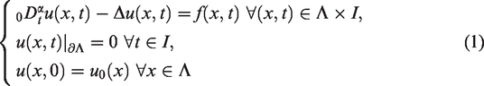
We consider the time fractional differential equations as follows:

{\begin{array}{l} _{0} D_{t}^{α} u (x, t) - Δ u (x, t) = f (x, t) \forall (x, t) \in Λ \times I, \\ u (x, t) |_{\partial Λ} = 0 \forall t \in I, \\ u (x, 0) = u_{0} (x) \forall x \in Λ \end{array}

(1)

where

Λ : = (a, b), I = (0, T], 0 < α < 1

, f is a given function. The left Caputo derivative of order α,

_{0} D_{t}^{α}

, are defined by¹

_{0} D_{t}^{α} u (x, t) : = g_{α} \int_{0}^{t} \frac{\partial_{s} u (x, s)}{{(t - s)}^{α}} d s

where

g_{α} = \frac{1}{Γ (1 - α)}

, and

Γ (\cdot)

is the Gamma function.

The presence of the integral in the equation makes the problem “global time dependence”. This means that the solution at a time t_k depends on the solutions at all previous time $t < t_{k}$ . The fact that all previous solutions have to be used to compute the solution at the current time level would make the storage very expensive if a low-order method is employed. To overcome the difficulties caused by the low-order methods, some high accuracy methods have been proposed to solve such type of “global time dependence” problems, such as spectral methods,^2–7 spectral element methods (SEM)^5,8 and references therein. However, the resulted linear system of the SM or SEM is dense due to the non-locality of the fractional operators and the condition number may grow fast. Furthermore, the required number of degrees of the freedom may be rather large due to the singularity of the solutions of FDEs, especially for a time-dependent problem.

To resolve this important issue, we adopt the idea of the time parallel method. The parallel in time algorithm for a model ODE was initially introduced by Lions, Maday, and Turinici⁹ as a numerical method to solve the evolution problems in parallel. It can be interpreted as a predictor-corrector scheme,^10,11 which involves a prediction step based on a coarse approximation and a correction step computed in parallel based on a fine approximation. For the parallel in time method based on the finite difference scheme, the convergence analysis for a ODE problem was given in Gander and Vandewalle.¹² For high accuracy parallel method, Li, Tang and Xu¹³ proposed a time parallel based on spectral method for Volterra integral equations and exponential convergence was proved. Xu et al.¹⁴ proposed a time parallel method based on spectral method for TFDEs.

In this work, we propose a parallel in time method based on a spectral collocation scheme and a finite difference method for the TFDEs. The main goal of this method is to parallelize the time discretization to obtain an important speed up which makes it possible to consider the really long integration problems. The method consists in splitting the time domain into a set of subdomains, and breaking the original problem into a series of independent problems on the time subdomains. The key point of this method lies in the design of an efficient iterative process while each step containing a predictor and a corrector solvers. The predictor is solved by a coarse finite difference approximation. Corrector is solved by computing difference between the fine spectral collocation approximation and the finite difference approximation in parallel way. Here, the finite difference method we adopt in parallel method was proposed by Lin.¹⁵ The convergence of the finite difference method was proved to be ${(δ t)}^{2 - α}$ on the time direction. Some numerical tests implemented on the parallel machine are carried out to test the precision of the method and the efficiency of the proposed method.

This paper is organized as follows. In section 2, we construct the parallel in time method based on the spectral collocation scheme and the finite difference method for the underlying equation. Numerical experiments are carried out in section 3. The efficiency for the proposed method under some assumptions is given in section 4.

The parallel in time algorithm

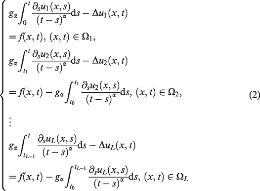
In order to describe the parallel method for problem (1), we separate the time interval $I = [0, T]$ into L subintervals, determined by the grid points

\begin{array}{l} 0 = t_{0} < t_{1} < t_{2} < \dots < t_{L} = T, \\ with t_{l} = l Δ t, Δ t = \frac{T}{L} \end{array}

(1)

We denote this partition by $I = \cup_{l = 1}^{L} I_{l}, I_{l} = [t_{l - 1}, t_{l}]$ .

Let $u = {(u_{1}, u_{2}, \dots u_{L})}^{T},$ where $u_{l} (x, t)$ is the solution of (1) on the l-th element, i.e., $u_{l} (x, t) = u (x, t), \forall (x, t) \in Ω_{l} : = Λ \times [t_{l - 1}, t_{l}], l = 1, \dots, L .$ It is readily seen that the following system of L separate initial value problems holds:

{\begin{array}{l} g_{α} \int_{0}^{t} \frac{\partial_{s} u_{1} (x, s)}{{(t - s)}^{α}} d s - Δ u_{1} (x, t) \\ = f (x, t), (x, t) \in Ω_{1}, \\ g_{α} \int_{t_{1}}^{t} \frac{\partial_{s} u_{2} (x, s)}{{(t - s)}^{α}} d s - Δ u_{2} (x, t) \\ = f (x, t) - g_{α} \int_{t_{0}}^{t_{1}} \frac{\partial_{s} u_{2} (x, s)}{{(t - s)}^{α}} d s, (x, t) \in Ω_{2}, \\ ⋮ \\ g_{α} \int_{t_{L - 1}}^{t} \frac{\partial_{s} u_{L} (x, s)}{{(t - s)}^{α}} d s - Δ u_{L} (x, t) \\ = f (x, t) - g_{α} \int_{t_{0}}^{t_{L - 1}} \frac{\partial_{s} u_{L} (x, s)}{{(t - s)}^{α}} d s, (x, t) \in Ω_{L} \end{array}

(2)

To simplify the notation, we introduce the operator $S_{l}$ , such that $u_{l} (x, t) = S_{l} (x, t, u_{l - 1}, \dots, u_{1})$ .

Let $F_{l}$ be the fine approximation to $S_{l}$ , which will be defined hereafter by a highly accurate spectral collocation method on element Ω _l . To this end, we define $P_{M} (Λ)$ (resp. $P_{N} (I_{l})$ ) as the polynomial spaces of degree less than or equal to M(resp. N) with respect to x(resp. t). Let $P_{M}^{0} (Λ) : = P_{M} (Λ) \cap_{H}^{01} (Λ)$ . Then we define the spectral approximation space as:

S_{M N} (Ω_{l}) : = P_{M}^{0} (Λ) \times P_{N} (I_{l})

Let $\bar{Λ} = [- 1, 1]$ . We denote by $J_{M}^{α, β} (x), - 1 \leq x \leq 1$ , the Jacobi polynomial of degree M associated with the weights $ω^{α, β} (x) = {(1 - x)}^{α} {(1 + x)}^{β}$ . Let $x_{m}^{α, β}$ be the points of the Gauss-Jacobi (GJ) quadrature formula, arranged by the increasing order: $- 1 < x_{0}^{α, β} < x_{1}^{α, β} < \dots < x_{M}^{α, β} < 1$ . The associated weights of the GJ quadrature formula are denoted by $ω_{m}^{α, β}, 0 \leq m \leq M$ . Then it is well-known the following identity:

\int_{\bar{Λ}} φ (x) d x = \sum_{m = 0}^{M} φ (x_{m}^{α, β}) ω_{m}^{α, β}, \forall φ \in P_{2 M + 1} (\bar{Λ})

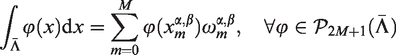
The discrete L² inner product associated to the GJ quadrature is denoted by:

{(φ, ψ)}_{M, ω^{α, β}} : = \sum_{m = 0}^{M} φ (x_{m}^{α, β}) ψ (x_{m}^{α, β}) ω_{m}^{α, β}

(3)

Furthermore, we define the Legendre-Gauss (LG) points on the element $I_{l} = [t_{l - 1}, t_{l}]$ , i.e.,

η_{l}^{n} = \frac{t_{l} - t_{l - 1}}{2} x_{n}^{0, 0} + \frac{t_{l} + t_{l - 1}}{2} 0 \leq n \leq N, 1 \leq l \leq L

and the corresponding weights

ρ_{l}^{n} = \frac{Δ t}{2} ω_{n}^{0, 0}, 0 \leq n \leq N, 1 \leq l \leq L

The LG points $ξ^{m}, 0 \leq m \leq M$ , on the element Λ are defined by a similar way.

Now the fine approximation $F_{l}$ are defined by the Legendre-collocation method for (2) as follows: find $U_{l} (x, t) \in S_{M N} (Ω_{l}), l = 1, \dots, L$ , such that, for all $0 \leq m \leq M, 0 \leq n \leq N$ ,

{\begin{array}{l} g_{α} \int_{0}^{η_{1}^{n}} \frac{\partial_{s} U_{1} (ξ^{m}, s)}{{(η_{1}^{n} - s)}^{α}} d s - Δ U_{1} (x, t) |_{(ξ^{m}, η_{1}^{n})} \\ = f (ξ^{m}, η_{1}^{j}), \\ g_{α} \int_{t_{1}}^{η_{2}^{n}} \frac{\partial_{s} U_{2} (ξ^{m}, s)}{{(η_{2}^{n} - s)}^{α}} d s - Δ U_{2} (x, t) |_{(ξ^{m}, η_{2}^{n})} \\ = f (ξ^{m}, η_{2}^{n}) - g_{α} \int_{t_{0}}^{t_{1}} \frac{\partial_{s} U (ξ^{m}, s)}{{(η_{2}^{n} - s)}^{α}} d s, \\ ⋮ \\ g_{α} \int_{t_{L - 1}}^{η_{L}^{n}} \frac{\partial_{s} U_{L} (ξ^{m}, s)}{{(η_{L}^{n} - s)}^{α}} d s - Δ U_{L} (x, t) |_{(ξ^{m}, η_{L}^{n})} \\ = f (ξ^{m}, η_{L}^{n}) - g_{α} \sum_{k = 1}^{L - 1} \int_{t_{k - 1}}^{t_{k}} \frac{\partial_{s} U_{k} (ξ^{m}, s)}{{(η_{L}^{n} - s)}^{α}} d s \end{array}

(4)

In the implementation, the integral terms on the left hand sides of (4) are evaluated by using the following Jacobi Gauss quadrature:

\begin{array}{l} \int_{t_{l - 1}}^{η_{l}^{n}} \frac{\partial_{s} U (ξ^{m}, s)}{{(η_{l}^{n} - s)}^{α}} d s \\ = {(\frac{η_{l}^{n} - t_{l - 1}}{2})}^{- α} \int_{- 1}^{1} \partial_{y} U (ξ^{m}, s_{l}^{n}) (1 - y)^{- α} d y \\ \approx {(\frac{η_{l}^{n} - t_{l - 1}}{2})}^{- α} {(\partial_{y} U (ξ^{m}, s_{l}^{n}), 1)}_{N, ω^{- α, 0}} \end{array}

where

s_{l}^{n} (y) = \frac{η_{l}^{n} - t_{l - 1}}{2} y + \frac{η_{l}^{n} + t_{l - 1}}{2}

The right hand sides of (4) are computed in a similar way:

\begin{array}{l} \int_{t_{l - 1}}^{t_{l}} \frac{\partial_{s} U (ξ^{m}, s)}{{(η_{l}^{n} - s)}^{α}} d s \\ = \int_{- 1}^{1} \partial_{y} U (ξ^{m}, s_{l} (y)) (η_{l}^{n} - s_{l} (y))^{- α} d y \\ \approx {(\partial_{y} U (ξ^{m}, s_{l}), {(η_{l}^{n} - s_{l} (y))}^{- α})}_{N, ω^{0, 0}}, \end{array}

where

s_{l} (y) = \frac{t_{l} - t_{l - 1}}{2} y + \frac{t_{l} + t_{l - 1}}{2}, - 1 < y < 1.

(5)

We will use the operators $F_{l}$ to denote (4) combined with the above approximations, i.e., $U_{l} (x, t) = F_{l} (x, t, U_{l - 1}, U_{l - 2}, \dots, U_{1}), t \in [t_{l - 1}, t_{l}]$ . Clearly, the above process is sequential since $U_{l - 1}, U_{l - 2}, \dots$ , and U₁ are needed to compute U_l.

In addition to the fine approximations $F_{l}$ , the parallel in time method assumes we are given another coarse approximation operator, denoted by .., which is cheaper (and consequently less accurate) than $F_{l}$ . For the time direction, we apply the finite difference method proposed by Lin et al.¹⁵ To this end, we introduce another coarse grids in the following. Given an integer $q \geq 1$ , the local time interval $[t_{l - 1}, t_{l}]$ is divided into q intervals, and consequently the global time interval I is divided into Lq subintervals, i.e.,

t_{0} = {\tilde{t}}_{0} < {\tilde{t}}_{1} < \dots < {\tilde{t}}_{L q} = t_{L} = T, with {\tilde{t}}_{i} = i δ t, δ t = \frac{T}{L q}

Comparing this with partition (1), they coincide at the points $t_{i} = {\tilde{t}}_{q i}, 0 \leq i \leq L$ . Particularly, $t_{i} = {\tilde{t}}_{i}, δ t = Δ t$ , if q = 1.

For $1 \leq i \leq L q$ , the finite difference method for the time fractional operator is stated as:

\begin{array}{l} _{0} D_{{\tilde{t}}_{i}}^{α} u (x, {\tilde{t}}_{i}) = g_{α} \sum_{j = 1}^{i} \int_{{\tilde{t}}_{j - 1}}^{{\tilde{t}}_{j}} \frac{\partial_{s} u (x, s) d s}{{({\tilde{t}}_{i} - s)}^{α}} \\ = g_{α} \sum_{j = 1}^{i} \frac{u (x, {\tilde{t}}_{j}) - u (x, {\tilde{t}}_{j - 1})}{δ t} \int_{{\tilde{t}}_{j - 1}}^{{\tilde{t}}_{j}} \frac{d s}{{({\tilde{t}}_{i} - s)}^{α}} \\ = \frac{g_{α}}{1 - α} \sum_{j = 1}^{i} \frac{u (x, {\tilde{t}}_{j}) - u (x, {\tilde{t}}_{j - 1})}{δ t^{α}} \\ \cdot [{(i + 1 - j)}^{1 - α} - {(i - j)}^{1 - α}] + r_{α}^{i} \\ = \frac{g_{α}}{1 - α} \sum_{j = 1}^{i} a_{j} \frac{u (x, {\tilde{t}}_{i + 1 - j}) - u (x, {\tilde{t}}_{i - j})}{δ t^{α}} + r_{α}^{i} \end{array}

(6)

where

a_{j} = j^{1 - α} - {(j - 1)}^{1 - α}, r_{α}^{i} \leq c δ t^{2 - α}

Now we define the coarse solver $G_{l}$ by combining the above finite difference in time direction with the Legendre-collocation method in spacial direction for (2) as follows: find $V (x, {\tilde{t}}_{i}) \in P_{M}^{0} (Λ), i = 1, \dots, q L$ , such that, for all $0 \leq m \leq M$ ,

\begin{array}{l} \frac{g_{α}}{(1 - α) δ t^{α}} V (ξ^{m}, {\tilde{t}}_{i}) - Δ V (ξ^{m}, {\tilde{t}}_{i}) \\ = f (ξ^{m}, {\tilde{t}}_{i}) + \sum_{j = 1}^{i - 1} (a_{j} - a_{j + 1}) V (ξ^{m}, {\tilde{t}}_{i - j}) \\ + a_{i} V (ξ^{m}, {\tilde{t}}_{0}) . \end{array}

(7)

Then the parallel in time algorithm proposes an approximation to each $U_{l} (x, t), l = 1, \dots, L$ , as the limit of the sequence $U_{l}^{k} (x, t)$ defined by

\begin{array}{l} U_{l}^{k} = G_{l} (t, U_{l - 1}^{k}, U_{l - 2}^{k}, \dots, U_{1}^{k}) \\ + F_{l} (t, U_{l - 1}^{k - 1}, U_{l - 2}^{k - 1}, \dots, U_{1}^{k - 1}) \\ - G_{l} (t, U_{l - 1}^{k - 1}, U_{l - 2}^{k - 1}, \dots, U_{1}^{k - 1}), k \geq 1, \end{array}

(8)

with the initial value:

U_{l}^{0} = G_{l} (t, U_{l - 1}^{0}, U_{l - 2}^{0}, \dots,_{U}^{10}),

(9)

where the subscript l refers to the element number, the supscript k refers to the iteration number, and

U_{l}^{k} (t)

represents an approximation of the solution

U_{l} (t)

at the time interval

[t_{l - 1}, t_{l}]

It is an easy matter to realize first that the method is exact after enough iterations. Indeed, by induction we obtain that $U_{l}^{l} = U_{l}$ for any l > 0. However our numerical experiments in Figure 4 show that the convergence of $U_{l}^{k}$ to U_l goes much faster as we shall see shortly.

Numerical results

In this section, we present some numerical results obtained by the proposed parallel in time scheme. First, we test the convergence behavior with respect to some parameters of the approximation. Second, we test the efficiency of the parallel iterative scheme.

We consider the following example:

_{0} D_{t}^{α} u (x, t) - Δ u (x, t) = f (x, t) \forall (x, t) \in [0, 1] \times [0, T],

(10)

with the exact solution

u (x, t) = sin (π x) sin (π t)

and

α = 0.5

. The first purpose is to investigate the convergence behavior of the numerical solutions with respect to the polynomial degrees M, N, the iteration number k and the parameter q for the coarse grids. In the top of Figure 1, we plot the

L^{\infty}

-errors in semi-log scale as a function of N with M = 15, iteration number k = 20, time domain T = 30, q = 1. The domain is partitioned into 30 subintervals,

Δ t = δ t

. In order to separate different error sources, the solution is computed after large enough iteration steps such that the error produce by the coarse solver is negligible as compared with the error of the fine resolution. As expected, the errors show an exponential decay, since in this semi-log representation one observes that the error variations are linear versus the degrees of polynomial N. Similarly, from bottom of the Figure 1, one observes the errors show an exponential decay versus the degrees of polynomial M.

Figure 1.

Top: $L^{\infty}$ -errors versus N with M = 15, k = 20, T = 30, L = 30, q = 1. Bottom: $L^{\infty}$ -errors versus M with N = 15, k = 20, T = 30, L = 30, q = 1.

Next we investigate the convergence behavior with respect to the iteration number k. For a similar reason mentioned above, we now fix a large enough M = 15, N = 15, and let k vary for different values of q. In Figure 2, we plot the error decay with increasing iteration number k for several values of q. It is observed that the error curves are all straight lines in this semi-log representation, which means the convergence of order k with respect to the error associated to the coarse resolution.

Figure 2.

$L^{\infty}$ -errors versus k with M = 15, N = 15, T = 30,L = 30, q = 1, 2, 4.

In Figure 3, we test the convergence behavior with respect to q in log-log scale for three iteration number k = 2, 3, 5. The errors show an algebraic decay, since in this log-log representation one observes that the error variations are linear versus $q = \frac{Δ t}{δ t}$ .

Figure 3. $L^{\infty}$ -errors versus q with $M = N = 15,$ T = 30, L = 30.

The second purpose is to test the efficiency of the scheme in a parallel machine. In the top of Figure 4, for fixed error less than $10^{- 12}$ , we compare the CPU time of iterative scheme in parallel machine with the CPU time of the fine solver in single processor. The blue line shows the time cost with respect to the number of parallel elements L for solving the problem by scheme (8) while the red line shows CPU time cost for solving the problem by spectral collocation method in sequential way. Mean while, in the bottom of Figure 4, we plot the iteration number corresponding to blue line in the left of Figure 4 for fixed error less than $10^{- 12}$ . One observes that the iteration number keeps constant while the number of elements grow larger.

Figure 4.

For fixed $L_{\infty}$ error less then $10^{- 12}, M = 15, N = 38, Δ t = 10, q = 10.$ Top: CPU time versus the number of parallel elements L, $T = L Δ t$ . Bottom: iteration number versus the number of parallel elements L, $T = L Δ t$ .

Parallelism efficiency

Firstly, the classical sequential scheme based on the fine mesh consists of solving the problems $F_{l} (t, U_{l - 1}, U_{l - 2}, \dots, U_{1})$ consecutively for $l = 1, 2, \dots, L$ . The computational complexity is equal to the sum of all the elementary operations in $I_{l}, l = 1, 2, \dots, L$ . Let’s denote the total computational cost by $C_{F}$ and the cost for l-th subproblem by $C_{F}^{l}$ , then $C_{F} = \sum_{l = 1}^{L} C_{F}^{l}$ . For the l-th subproblem, spectral discretization $F_{l}$ consists of evaluating the integral terms on the right hand sides and solving the linear system. The cost of evaluating the integral terms on the right hand sides approximately equal to $O (l N^{2} M)$ , while the cost for solving the linear system approximately equal to $O ((M^{2} + N^{2}) M N)$ , where $O (M^{2} + N^{2})$ is the number of operations needed for the matrix vector multiplication and $O (M N)$ is the estimated iteration number required to achieve the convergence of the iterative method. Then $C_{F}^{l} = O ((M^{2} + N^{2}) M N) + O (l N^{2} M)$ . As a result, the total computational complexity of the sequential fine solutions is

C_{F} = O ((M^{2} + N^{2}) MNL) + O (L^{2} N^{2} M)

(11)

If we implement the scheme (8) in a parallel architecture with enough processors, then for each iteration, the time cost of the master process consists of the computational time for solving a sequential set of L coarse subproblems and the waiting time for solving a fine subproblem on a non-master process. For the coarse subproblem, we apply the finite difference scheme (6) for the time discretization and the spectral method for space discretization. The cost of solving the sequential set of L coarse subproblems is estimated to be $\sum_{l = 1}^{L} C_{G}^{l}$ , where $C_{G}^{l} = O (M^{3} q)$ is the cost to solve the l-th coarse subproblem. The cost of solving a single fine subproblem is approximately $O ((M^{2} + N^{2}) M N) + O (l N^{2} M)$ . Note also, in the implementation of the parallel in time scheme there is a need to interpolate the solution between the fine mesh and coarse mesh, the cost of which is $O (LMNq)$ . Therefore if k is the number of iterations required to achieve the desired convergence of the parallel in time algorithm, then the total computational complexity is

k [O (M^{3} q L) + O ((M^{2} + N^{2}) M N) + O (L N^{2} M) + O (LMNq)]

(12)

Comparing (11) with (12), we obtain a speed up

\frac{k [O (M^{3} q L) + O ((M^{2} + N^{2}) M N) + O (L N^{2} M) + O (LMNq)]}{O ((M^{2} + N^{2}) MNL) + O (L^{2} N^{2} M)}

If the number of processors is large enough, i.e., $L > > M, L > > N$ , and the number of degrees of freedom for the coarse solver is far less than that of the fine solver which means q is small, then the speed up is close to $O (\frac{k}{L})$ . From the right of Figure 4, we observe that the iteration number k keeps constant while the number of elements L grow larger.

Conclusions

We propose a parallel in time method, combined with the spectral collocation scheme and the finite difference scheme for the TFDEs. As the domain decomposition method, we break the domain of computation into L subdomains and thus the problem is divided into L sub-problems consequently. Then we solve these sub-problems by a predictor-corrector scheme in a parallel way. The predictor is solved by a cheap coarse approximation based on the finite difference method in sequential way, while the corrector is solved by the expensive fine approximation based on the spectral collocation method in parallel way. Numerical results are carried out to confirm the efficiency of the parallel method. The solution of the iterative scheme converges to the solution of the spectral method. The errors decay spectrally with respect to the polynomial degrees N and M, while the errors decay algebraically with respect to the parameter q of coarse approximation. The convergence of order k (iteration number) with respect to the error associated to the solution solved by the finite difference method is given in Figure 2. In Figure 4, the CPU time cost is compared between the parallel scheme and the sequential scheme based on the spectral collocation method. The efficiency analysis of the proposed method is given. If the number of processors is large enough, and the number of degrees of freedom for the coarse solver is far less than that of the fine solver which means q is small, then the speed up is close to $O (\frac{k}{L})$ . In the future work, we will try to analyze the convergence of the parallel method for the fractional differential equations theoretically.

Footnotes

Declaration of conflicting interests

The author(s) declared no potential conflicts of interest with respect to the research, authorship, and/or publication of this article.

Funding

The author(s) disclosed receipt of the following financial support for the research, authorship, and/or publication of this article: This article is supported by NSFC, grant no. 11771083 and NSF of Fuzhou University through grant GXRC-18035.

ORCID iD

Xianjuan Li

References

Podlubny

Fractional differential equations: an introduction to fractional derivatives, fractional differential equations, to methods of their solution and some of their applications. Amsterdam: Elsevier, 1998.

A space-time spectral method for the time fractional diffusion equation. SIAM J Numer Anal 2009; 47: 2108–2131.

Existence and uniqueness of the weak solution of the space-time fractional diffusion equation and a spectral method approximation. CiCP 2010; 8: 1016–1051.

Mao

Chen

Shen

Efficient and accurate spectral method using generalized Jacobi functions for solving Riesz fractional differential equations. Appl Numer Math 2016; 106: 165–181.

Mao

Karniadakis

GE.

A spectral method (of exponential convergence) for singular solutions of the diffusion equation with general two-sided fractional derivative. SIAM J Numer Anal 2018; 56: 24–49.

Mao

Shen

Efficient spectral–Galerkin methods for fractional partial differential equations with variable coefficients. J Comput Phys 2016; 307: 243–261.

Zayernouri

Karniadakis

GE.

Fractional Sturm–Liouville Eigen-problems: theory and numerical approximation. J Comput Phys 2013; 252: 495–517.

Zayernouri

Karniadakis

GE.

Discontinuous spectral element methods for time-and space-fractional advection equations. SIAM J Sci Comput 2014; 36: B684–B707.

Lions

Maday

Turinici

Résolution d’EDP par un schéma en temps ğpararéel ğ: A. Comptes Rendus de L’Académie Des Sciences-Series I-Mathematics 2001; 332: 661–668.

10.

Bal

Parallelization in time of (stochastic) ordinary differential equations. Math Meth Anal Num 2003. https://www.researchgate.net/publication/237456541_PARALLELIZATION_IN_TIME_OF_STOCHASTIC_ORDINARY_DIFFERENTIAL_EQUATIONS

11.

Bal

Maday

A parareal time discretization for non-linear PDEs with application to the pricing of an American put. In: Proceedings of the workshop on domain decomposition, LNCSE Series 2001; 23:189–201.

12.

Gander

Vandewalle

Analysis of the parareal time-parallel time-integration method. SIAM J Sci Comput 2007; 29: 556–578.

13.

Tang

Parallel in time algorithm with spectral-subdomain enhancement for volterra integral equations. SIAM J Numer Anal 2013; 51: 1735–1756.

14.

Hesthaven

Chen

A parareal method for time-fractional differential equations. J Comput Phys 2015; 293: 173–183.

15.

Lin

Finite difference/spectral approximations for the fractional cable equation. Math Comp 2010; 80: 1369–1396.

A parallel in time/spectral collocation combined with finite difference method for the time fractional differential equations

Abstract

Keywords

Introduction

The parallel in time algorithm

Numerical results

Parallelism efficiency

Conclusions

Footnotes

Declaration of conflicting interests

Funding

ORCID iD

References