Approximation of noisy data using multivariate splines and finite element methods

Abstract

We compare a recently proposed multivariate spline based on mixed partial derivatives with two other standard splines for the scattered data smoothing problem. The splines are defined as the minimiser of a penalised least squares functional. The penalties are based on partial differential operators, and are integrated using the finite element method. We compare three methods to two problems: to remove the mixture of Gaussian and impulsive noise from an image, and to recover a continuous function from a set of noisy observations.

Introduction

We begin by outlining the scattered data problem. Consider the set of scattered points $\mathcal{G}={\left\{{\mathbf{p}}_i\right\}}_{i=1}^N$ in a domain $\Omega \subseteq {ℝ}^d$ with $d\in \mathbb{N}$ , and the set of noisy observations at those points ${\left\{z_i\right\}}_{i=1}^N$ . We want to reconstruct an unknown function u to approximate the given data. Assuming that the underlying data set is corrupted with Gaussian noise, we can assume that the unknown function u satisfies

$$z_i=u({\mathbf{p}}_i)+n_i$$

$i=1,\dots N$ , where ${\left\{n_i\right\}}_{i=1}^N$ is a set of normally distributed random variables with mean 0 and variance ${\sigma }^2$ .

To recover the unknown function u, we will use an approach based on the multivariate L-spline. That is, we will search for a function u that minimises the following least squares functional

$${\displaystyle \sum _{i=1}^N(z_i-u(}{\mathbf{p}}_i){)}^2+\lambda {\displaystyle {\int }_{\Omega }(Lu(}x,y){)}^2\mathrm{d}\mathbf{x}$$

over a Sobolev space V, where L is a partial differential operator, and λ is a positive smoothing parameter.

We use the standard notation for Sobolev spaces on Ω.^1–3 We consider three different choices for L. The first choice is to take Lu as the gradient of u. Then we need to have $V=H^1(\Omega )$ . However, the continuous problem is not well-posed with this choice for $d\ge 2$ , because the point value of a function is not defined in $H^1(\Omega )$ when $d\ge 2$ . The second choice is to choose Lu as the Laplacian of u. Then we need to have $V=H^2(\Omega )$ . Again, the continuous problem is not well-posed for d > 3, because the point value of a function is not defined in $H^2(\Omega )$ when d > 3. The third choice is to include mixed partial derivatives of u on the gradient penalty to construct Lu. ⁴ Unlike the other two choices, the resulting spline is well defined for any dimension $d\in \mathbb{N}$ .

This is the first time that computational results of the newly proposed multivariate spline ⁴ are presented and compared with other existing techniques. Moreover, we observe the instability of the gradient penalty approach in our numerical experiments, which is another novelty of this contribution.

We will apply these methods to two problems. The first problem is to recover an image that have been corrupted with both Gaussian and impulsive noise. We apply a finite element method to compute the solution of the above minimisation problem. Finite element methods have recently become popular in different areas of image processing.^5–9 Finite element methods are applied in Lamichhane ¹⁰ and Lamichhane ¹¹ to remove the mixture of Gaussian and impulsive noise using the gradient penalty and total variation penalty, respectively.

The second problem is to recover a continuous function from a set of noisy observations. We consider observations that have been corrupted with Gaussian noise. In this example, we see spurious spikes in the solution using the gradient penalty. This is due to the fact that the gradient penalty does not control the point-wise values of the function. Numerical results show that we can increase the mesh-size to reduce the height of the spikes but they cannot be totally removed.

This paper is organised as follows. In the next section, we present the gradient penalty smoothing technique. In the third section, we present the smoothing technique based on the minimisation of a functional involving mixed partial derivatives. In the fourth section, we compare the three finite element methods in denoising images and recovering continuous functions. We discuss these results in the last section.

Multivariate spline with gradient penalty

The multivariate spline with the gradient penalty is given by the following minimisation problem

$$\underset{u\in V}{\min }\left({\displaystyle \sum _{i=1}^N(u(}{\mathbf{p}}_i)-z_i{)}^2+\lambda {\displaystyle {\int }_{\Omega }{\Vert \nabla u\Vert }^2}\mathrm{d}\mathbf{x}\right)$$

(1)

Due to the choice of the minimisation functional it is natural to take $V=H^1(\Omega )$ , for which the problem will not be well-posed when d > 1.

Now we consider a finite element discretisation of the spline. Let $C^0(\Omega )$ be the space of continuous functions in Ω and ${\mathcal{T}}_h$ a finite element triangulation of Ω. Note that ${\mathcal{T}}_h$ is the set of triangles or rectangles. Then let

$$V_h=\{u_h\in C^0(\Omega )|u_h{|}_T\in P(T),T\in {\mathcal{T}}_h\}$$

(2)

be a finite element space, where P(T) is the linear polynomial space if T is a triangle, and P(T) is the bilinear polynomial space on T if T is a rectangle. ¹² The minimisation problem leads to the variational problem of finding $u_h\in V_h$ such that

$$a(u_h,v_h)=\ell (v_h),v_h\in V_h$$

where the bilinear form $a(·,·)$ and the linear form $\ell (·)$ are given by

$$\begin{array}{l}a(u,v)={\displaystyle \sum _{i=1}^{N}u}({\mathbf{p}}_i)v({\mathbf{p}}_i)+\lambda {\displaystyle {\int }_{\Omega }\nabla }u·\nabla v\mathrm{d}\mathbf{x}\\ \ell (v)={\displaystyle \sum _{i=1}^{N}v}({\mathbf{p}}_i)z_i\end{array}$$

It is easy to show that the above problem has a unique solution under the assumption that the set of scattered points $\mathcal{G}$ is non-empty. ¹⁰

Since $a(·,·)$ is positive definite, we can define the energy ${\Vert ·\Vert }_a$ on V as

$${\Vert v\Vert }_a^2=a(v,v)$$

for all $v\in V$

The following lemma shows that the discrete multivariate spline with the gradient penalty is well-posed for d = 1 but not well-posed for d > 1. The point-value of a function is not controlled by the gradient of the function when d > 1. The well-posedness is exhibited in the stability result first proved in Garcke and Hegland. ¹³ For completeness we have given these results in Lemmas 1, 2 and 3, which are taken from Garcke and Hegland. ¹³

Lemma 1. (Discrete Sobolev inequality). There exists constant $c_d>0$ such that for all $u\in V_h$

$\left|u(x)\right|\le c_d{\Vert u\Vert }_{H^1(\Omega )}$ for d = 1.

$\left|u(x)\right|\le c_d\left(1+\left|\log h\right|\right){\Vert u\Vert }_{H^1(\Omega )}$ for d = 2.

$\left|u(x)\right|\le c_d{h}^{1-d/2}{\Vert u\Vert }_{H^1(\Omega )}$ for d > 2.

The constant c_d is independent of the mesh-size h but depends on d. These bounds are tight, and for d > 2 we have that

$$c_d\ge \frac{1}{\sqrt{3d+1}}{\left(\frac{3}{2}\right)}^{d/2}$$

Lemma 2. (Discrete Poincaré inequality). Let $(x_0,y_0)\in \Omega$ and $u_0=u(x_0,y_0)$ for $u\in V_h$ . Then there exist constants $c_d>0$ such that

${\Vert u-u_0\Vert }_{L^2(\Omega )}\le c_d{\Vert \nabla u\Vert }_{L^2(\Omega )}$ for d = 1

${\Vert u-u_0\Vert }_{L^2(\Omega )}\le c_d\left(1+\left|\log h\right|\right){\Vert \nabla u\Vert }_{L^2(\Omega )}$ for d = 2

${\Vert u-u_0\Vert }_{L^2(\Omega )}\le c_d{h}^{1-d/2}{\Vert \nabla u\Vert }_{L^2(\Omega )}$ for d > 2.

Lemma 3. (Discrete V-ellipticity). There exist constants c_d and C_d such that the energy norm on V_h satisfies

$${\alpha }_{d,h}{\Vert u\Vert }_{H^1(\Omega )}\le {\Vert u\Vert }_a\le {\beta }_{d,h}{\Vert u\Vert }_{H^1(\Omega )}$$

for all $u\in V_h$ , where ${\alpha }_{d,h}$ and ${\beta }_{d,h}$ are given by

1. ${\alpha }_{d,h}={\left(\frac{c_d}{\sqrt{\lambda }}+\frac{1}{\sqrt{\lambda }}+1\right)}^{-1}$ and ${\beta }_{d,h}=C_d+\sqrt{\lambda }$ for d = 1

2. ${\alpha }_{d,h}={\left(\frac{c_d\left(1+\left|\log h\right|\right)}{\sqrt{\lambda }}+\frac{1}{\sqrt{\lambda }}+1\right)}^{-1}$ and ${\beta }_{d,h}=C_d\left(1+\left|\log h\right|\right)+\sqrt{\lambda }$ for d = 2

3. ${\alpha }_{d,h}={\left(c_d{\lambda }^{-1/2}{h}^{1-d/2}+{\lambda }^{-1/2}+1\right)}^{-1}$ and ${\beta }_{d,h}=C_d{h}^{1-d/2}+\sqrt{\lambda }$ for d > 2.

The above results imply that for the solution $u_h\in V_h$ of the spline with the gradient penalty we have

$${\Vert u_h\Vert }_a\le \frac{{\beta }_{d,h}}{{\alpha }_{d,h}}{\Vert \ell \Vert }_{L^2(\Omega )}$$

where ${\Vert \ell \Vert }_{L^2(\Omega )}$ is the L²-norm of the linear functional $\ell$ .

Remark 4. We can see that the ill-posedness is exhibited in the stability constant being not independent of the mesh-size h. There is no easy way to remove this dependency.

Multivariate spline with Laplacian penalty

The multivariate spline with the Laplacian penalty is the solution of the following minimisation problem

$$\underset{u\in V}{\min }\left({\displaystyle \sum _{i=1}^N(u(}{\mathbf{p}}_i)-z_i{)}^2+\lambda {\displaystyle {\int }_{\Omega }{(\Delta u)}^2}\mathrm{d}\mathbf{x}\right)$$

(3)

where $V=H^2(\Omega )$ . The minimisation problem is well-posed for $d\in \{1,2,3\}$ since $H^2(\Omega )\subset C^0(\Omega )$ when $d\in \{1,2,3\}$ . More details of this spline can be found in Ramsay. ¹⁴ This spline will be called Laplacian spline in the following.

Remark 5. The Laplacian penalty imposes higher smoothness in the solution. Since we look for a solution, whose second derivatives are square integrable, point-values of the solution are well-defined in contrast to the gradient penalty spline. However, a finite element approximation of the Laplacian spline is more expensive than the gradient penalty spline.

While we can use a direct finite element approximation using a low order finite element space V_h to approximate the gradient penalty spline, we cannot directly use this space to approximate the Laplacian spline as $\Delta u_h$ for $u_h\in V_h$ is not well-defined. We use a mixed finite element method proposed by Lamichhane. ¹⁵ We first introduce a new variable $\varphi =\Delta u$ in the minimisation formulation (3) and then write a weak equation as

$${\displaystyle {\int }_{\Omega }\varphi }\mu \mathrm{d}\mathbf{x}={\displaystyle {\int }_{\Omega }\nabla }u·\nabla \mu \mathrm{d}\mathbf{x},\mu \in H^1(\Omega )$$

(4)

Now choosing $\varphi \in L^2(\Omega )$ and $u,\mu \in H^1(\Omega )$ , we have a well-defined formulation for which we can use the space V_h to discretise u and μ, whereas we use a discontinuous piecewise polynomial space W_h to discretise $\varphi$ . The basis functions of W_h and V_h satisfy a biorthogonality relationship ¹⁵ so that the associated matrix corresponding to the L²-inner product ${\int }_{\Omega }\varphi \mu dx$ in (4) is diagonal. In this way, we arrive at a very efficient finite element method to approximate the solution of the minimisation problem (3). The discrete problem is then to compute

$$\underset{[u_h,{\varphi }_h]\in V_h\times W_h}{\min }\left({\displaystyle \sum _{i=1}^N(u_h(}{\mathbf{p}}_i)-z_i{)}^2+\lambda {\displaystyle {\int }_{\Omega }{\varphi }_h^2}\mathrm{d}\mathbf{x}\right)$$

subject to the constraint

$${\displaystyle {\int }_{\Omega }{\varphi }_h}{\mu }_h\mathrm{d}\mathbf{x}={\displaystyle {\int }_{\Omega }\nabla }{u}_h·\nabla {\mu }_h\mathrm{d}\mathbf{x},{\mu }_h\in V_h$$

Since $C^0(\Omega )\cancel{\subset }{H}^1(\Omega )$ when d > 1, the gradient penalty spline formulation does not provide a well-posed problem. The problem is well-posed only in one dimension. Similarly, $C^0(\Omega )\subset H^2(\Omega )$ for $d\in \{1,2,3\}$ but $C^0(\Omega )\cancel{\subset }{H}^2(\Omega )$ when d > 3. This motivates us to find a well-posed spline formulation for any $d\in \mathbb{N}$ , which is given in the next section.

New multivariate spline with mixed derivative penalty

In order to define the new multivariate spline, we define the associated Sobolev space. Let $\mathcal{B}={\{0,1\}}^d\backslash \left\{\mathbf{0}\right\}$ , where $\mathbf{0}\in {ℝ}^d$ is a zero vector. We use a standard multi-index notation with $\mathit{\alpha }=({\alpha }_1,\cdots ,{\alpha }_d)\in \mathcal{B}$ so that a mixed derivative of a sufficiently smooth function u is denoted by

$$D^{\mathit{\alpha }}u=\frac{{\partial }^{{\displaystyle {\sum }_{i=1}^d{\alpha }_i}}u}{\partial x_1^{{\alpha }_1}\cdots \partial x_d^{{\alpha }_d}}$$

where we use the usual Cartesian coordinate system with $\mathbf{x}=(x_1,\cdots ,x_d)\in {ℝ}^d$ .

We now define our Sobolev space for the multivariate spline problem as

$$H_m^1(\Omega ):=\left\{u\in L^2(\Omega ):D^{\mathit{\alpha }}u\in L^2(\Omega ),\mathit{\alpha }\in \mathcal{B}\right\}$$

which is equipped with the norm

$$\left|\right|u|{|}_{H_m^1(\Omega )}=\sqrt{\left|\right|u|{|}_{L^2(\Omega )}^2+{\displaystyle \sum _{\mathit{\alpha }\in \mathcal{B}}\left|\right|}{D}^{\mathit{\alpha }}u|{|}_{L^2(\Omega )}^2}$$

and the semi-norm

$$|u{|}_{H_m^1(\Omega )}=\sqrt{{\displaystyle \sum _{\mathit{\alpha }\in \mathcal{B}}\left|\right|}{D}^{\mathit{\alpha }}u|{|}_{L^2(\Omega )}^2}$$

The semi-norm for d = 2 is simply

$$|v{|}_{H_m^1(\Omega )}=\sqrt{{\displaystyle {\int }_{\Omega }{\Vert \nabla v\Vert }^2}+{\left(\frac{{\partial }^{2}v}{\partial x\partial y}\right)}^2\mathrm{d}\mathbf{x}}$$

where $\left|\right|\nabla v|{|}^2$ is the Euclidean norm of the vector $\nabla v\in {ℝ}^2$ .

We note that the space $H_m^1(\Omega )$ is a Hilbert space, and $H_m^1(\Omega )\subset C^0(\Omega )$ . ¹⁶ The new multivariate spline is then obtained as a solution of the minimisation problem

$$\underset{u\in H_m^1(\Omega )}{\min }\left({\displaystyle \sum _{i=1}^N(u(}{\mathbf{p}}_i)-z_i{)}^2+\lambda |u{|}_{H_m^1(\Omega )}^2\right)$$

(5)

The associated inner-product for the semi-norm on $H_m^1$ -space for d = 2 is

$${〈u,v〉}_{H_m^1(\Omega )}={\displaystyle {\int }_{\Omega }\nabla }{u}^T\nabla v+\frac{{\partial }^{2}u}{\partial x\partial y}\frac{{\partial }^{2}v}{\partial x\partial y}d\mathbf{x}$$

We can define a bilinear form $b(·,·)$ and a linear form $\ell (·)$ as

$$\begin{array}{l}b(u,v)=(Pu{)}^T(Pv)+\lambda 〈u,v{〉}_{H_m^1(\Omega )}\\ \ell (v)=(Pv{)}^T\mathbf{z}\end{array}$$

where

$$Pu={(u(x_1,y_1),u(x_2,y_2),\dots ,u(x_N,y_N))}^T$$

is a column vector of the function values of u at the scattered points $\mathcal{G}={\left\{{\mathbf{p}}_i\right\}}_{i=1}^N$ , and $\mathbf{z}\in {ℝ}^N$ is a column vector with ith component z_i. Then the multivariate spline problem is to find $u\in V$ such that

$$b(u,v)=\ell (v)$$

(6)

for all $v\in V$ .

Let Ω be a rectangle in ${ℝ}^2$ and ${\mathcal{T}}_h$ the tensor product partition of the domain with mesh size h, such that each element $T\in {\mathcal{T}}_h$ is a rectangle. Then we define a finite element space V_h as

$$V_h=\left\{u_h\in C^0(\Omega ):u_h{|}_T\in \mathcal{P}(T),T\in {\mathcal{T}}_h\right\},$$

where $\mathcal{P}(T)$ is the space of bilinear polynomials on T. We can now write our discrete multivariate spline problem as

$$\underset{u_h\in V_h}{\min }\left({\displaystyle \sum _{i=1}^N(u_h(}{\mathbf{p}}_i)-z_i{)}^2+\lambda |u_h{|}_{H_m^1(\Omega )}^2\right).$$

That is, the discrete problem is to find $u_h\in V_h$ such that

$$b(u_h,v_h)=\ell (v_h)$$

(7)

for all $v_h\in V_h$ .

The discrete problem is shown to be well-posed in Lamichhane. ¹¹ Here we recall some of the important results. We first show that the bilinear form $b(·,·)$ is positive definite on V_h.

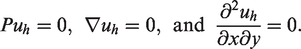
Lemma 6. Let $\lambda >0$ and let the set of scattered points $\mathcal{G}$ be non-empty. Then the bilinear form $b(·,·)$ is positive definite on the vector space V_h.

Proof. If u_h = 0, then clearly $b(u_h,u_h)=0$ . Conversely, let $b(u_h,u_h)=0$ . Then

$$P{u}_h=0, \nabla u_h=0,\text{ and }\frac{{\partial }^2{u}_h}{\partial x\partial y}=0.$$

Since u_h is a continuous function, $\nabla u_h=0$ gives that u is a constant function in Ω. Further, since $\mathcal{G}$ is non-empty and Pu_h = 0, we have that u_h = 0.

Since $b(·,·)$ is positive definite, we can define the energy norm ${\Vert ·\Vert }_b$ on V_h as

$${\Vert v_h\Vert }_b^2=b(v_h,v_h)$$

for all $v_h\in V_h$ . Since $b(·,·)$ and $\ell (·)$ satisfy the conditions of the Lax-Milgram lemma,^2,3 the unique minimiser is the solution of the discrete problem (7). In addition, the following holds.

Lemma 7. Let $\lambda >0$ and let $\mathcal{G}$ be non-empty. Then the discrete problem (7) admits a unique solution which depends continuously on the data with respect to the energy norm ${\Vert ·\Vert }_b$ .

Proof. We have that

$$\begin{array}{l}\left|b(u_h,v_h)\right|\le {\Vert u_h\Vert }_b{\Vert v_h\Vert }_b,\text{ and}\\ \left|\ell (v_h)\right|\le \Vert \mathbf{z}\Vert {\Vert v_h\Vert }_b\end{array}$$

for all $u_h,v_h\in V_h$ . Hence $b(·,·)$ and $\ell (·)$ are continuous on V_h. We also have that

$$b(u_h,u_h)={\Vert u_h\Vert }_b^2$$

for all $u_h\in V_h$ . Hence $b(·,·)$ is coercive on V_h. By the Lax-Milgram lemma,^2,3 there exists a unique solution u_h of the discrete problem 7. Additionally, the solution depends continuously on the data z.

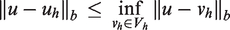
In addition, a direct application of the Céa lemma provides an optimal a priori estimate of the discrete solution.

Lemma 8. Let u be the solution to the continuous problem (6), and let u_h be the solution to the discrete problem (7). Then

$${\Vert u-u_h\Vert }_b\le \underset{v_h\in V_h}{\inf }{\Vert u-v_h\Vert }_b$$

Each finite element basis function is associated with a point in the tensor product partition ${\mathcal{T}}_h$ . Assuming there are mn points, we have mn basis functions. Let ${\left\{{\varphi }_i\right\}}_{i=1}^{mn}$ be the set of finite element basis functions, which span V_h. Then we can write our solution $u_h\in V_h$ as a linear combination of these basis functions, namely

$$u_h(x,y)={\displaystyle \sum _{i=1}^{mn}{u}_i}{\varphi }_i(x,y)$$

Let $\mathbf{u}={(u_1,u_2,\dots ,u_{mn})}^T$ and let K be the finite element stiffness matrix, where $K_{ij}={\int }_{\Omega }\nabla u_h^T\nabla v_{h}d\mathbf{x}$ . Let M be a mixed partial derivative matrix, where $M_{ij}={\int }_{\Omega }\frac{\partial u_h}{\partial x\partial y}\frac{\partial v_h}{\partial x\partial y}d\mathbf{x}$ . Then the finite element problem leads to the linear system

$$(A^{T}A+\lambda (K+M))\mathbf{u}=A^T\mathbf{z}$$

where A is a matrix of size N × mn, with entries $A_{ij}={\varphi }_j({\mathbf{p}}_i)$ .

Computation of K and M

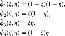
We will use a reference element to construct the matrices K and M. For rectangles, we choose our reference element $\widehat{T}$ to be the square with vertices $(0,0),(1,0),(1,1),$ and (0, 1). We then construct local basis functions at these vertices. These are

$$\begin{array}{l}{\widehat{\varphi }}_1(\xi ,\eta )=(1-\xi )(1-\eta ),\\ {\widehat{\varphi }}_2(\xi ,\eta )=\xi (1-\eta ),\\ {\widehat{\varphi }}_3(\xi ,\eta )=\xi \eta ,\\ {\widehat{\varphi }}_4(\xi ,\eta )=(1-\xi )\eta \end{array}$$

Now consider the rectangular element T with vertices $(x_1,y_1),(x_2,y_1),(x_2,y_2),$ and (x₁, y₂). We construct global basis functions at these vertices. When restricted to the element, these are given by

$$\begin{array}{l}{\varphi }_1(x,y)=\frac{(y-y_2)(x-x_2)}{(y_1-y_2)(x_1-x_2)},\\ {\varphi }_2(x,y)=\frac{(y-y_2)(x-x_1)}{(y_1-y_2)(x_2-x_1)},\\ {\varphi }_3(x,y)=\frac{(y-y_1)(x-x_1)}{(y_2-y_1)(x_2-x_1)},\\ {\varphi }_4(x,y)=\frac{(y-y_1)(x-x_2)}{(y_2-y_1)(x_1-x_2)}\end{array}$$

Let $F_T:\widehat{T}\to T$ be the bijective map from the reference element to T. This mapping is given by

$$\left[\begin{array}{l}x\\ y\end{array}\right]=\left[\begin{array}{ll}{x}_2-x_1& 0\\ 0& y_2-y_1\end{array}\right]\left[\begin{array}{l}\xi \\ \eta \end{array}\right]+\left[\begin{array}{l}{x}_1\\ y_1\end{array}\right]$$

Let the matrix in this transformation be denoted B_T. We note that ${\varphi }_i={\widehat{\varphi }}_i\mathrm{\hspace{0.17em}o\hspace{0.17em}}{F}_T^{-1}$ .

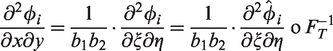
We will use the chain rule to calculate the derivatives. We have

$$\begin{array}{l}\frac{\partial {\varphi }_i}{\partial x}=\frac{1}{b_1}·\frac{\partial {\varphi }_i}{\partial \xi }=\frac{1}{b_1}·\frac{\partial {\widehat{\varphi }}_i}{\partial \xi }\mathrm{\hspace{0.17em}o\hspace{0.17em}}{F}_T^{-1},\\ \frac{\partial {\varphi }_i}{\partial y}=\frac{1}{b_2}·\frac{\partial {\varphi }_i}{\partial \eta }=\frac{1}{b_2}·\frac{\partial {\widehat{\varphi }}_i}{\partial \eta }\mathrm{\hspace{0.17em}o\hspace{0.17em}}{F}_T^{-1}\end{array}$$

where $b_1=x_2-x_1$ and $b_2=y_2-y_1$ .

Applying the chain rule again we obtain

$$\frac{{\partial }^2{\varphi }_i}{\partial x\partial y}=\frac{1}{b_1{b}_2}·\frac{{\partial }^2{\varphi }_i}{\partial \xi \partial \eta }=\frac{1}{b_1{b}_2}·\frac{{\partial }^2{\widehat{\varphi }}_i}{\partial \xi \partial \eta }\mathrm{\hspace{0.17em}o\hspace{0.17em}}{F}_T^{-1}$$

Now, we’ll calculate K. Let $K_T\in {ℝ}^{4\times 4}$ be the local stiffness matrix associated with the element T. Then

$${(K_T)}_{ij}={\displaystyle {\int }_T\frac{\partial {\varphi }_i}{\partial x}}·\frac{\partial {\varphi }_j}{\partial x}+\frac{\partial {\varphi }_i}{\partial y}·\frac{\partial {\varphi }_j}{\partial y}\mathrm{d}\mathbf{x}$$

Now

$$\begin{array}{l}{\displaystyle {\int }_T\frac{\partial {\varphi }_i}{\partial x}}·\frac{\partial {\varphi }_j}{\partial x}\mathrm{d}\mathbf{x}={\displaystyle {\int }_{\widehat{T}}\left(\frac{\partial {\varphi }_i}{\partial x}\mathrm{\hspace{0.17em}o\hspace{0.17em}}{F}_T\right)}\left(\frac{\partial {\varphi }_j}{\partial x}\mathrm{\hspace{0.17em}o\hspace{0.17em}}{F}_T\right)\left|\text{det}{B}_T\right|\mathrm{d}\widehat{\mathbf{x}}\\ =\frac{\left|\text{det}{B}_T\right|}{b_1^2}{\displaystyle {\int }_{\widehat{T}}\frac{\partial {\widehat{\varphi }}_i}{\partial \xi }}·\frac{\partial {\widehat{\varphi }}_j}{\partial \xi }\mathrm{d}\widehat{\mathbf{x}}=\frac{y_2-y_1}{x_2-x_1}{\displaystyle {\int }_{\widehat{T}}\frac{\partial {\widehat{\varphi }}_i}{\partial \xi }}·\frac{\partial {\widehat{\varphi }}_j}{\partial \xi }\mathrm{d}\widehat{\mathbf{x}}\end{array}$$

Similarly

$${\displaystyle {\int }_T\frac{\partial {\varphi }_i}{\partial y}}·\frac{\partial {\varphi }_j}{\partial y}\mathrm{d}\mathbf{x}=\frac{x_2-x_1}{y_2-y_1}{\displaystyle {\int }_{\widehat{T}}\frac{\partial {\widehat{\varphi }}_i}{\partial \eta }}·\frac{\partial {\widehat{\varphi }}_j}{\partial \eta }\mathrm{d}\widehat{\mathbf{x}}$$

Hence we have

$$\begin{array}{l}{K}_T=\frac{y_2-y_1}{6(x_2-x_1)}\left[\begin{array}{llll}2& -2& -1& 1\\ -2& 2& 1& -1\\ -1& 1& 2& -2\\ 1& -1& -2& 2\end{array}\right]\\ +\frac{x_2-x_1}{6(y_2-y_1)}\left[\begin{array}{llll}2& 1& -1& -2\\ 1& 2& -2& -1\\ -1& -2& 2& 1\\ -2& -1& 1& 2\end{array}\right]\end{array}$$

We then assemble each K_T into the global stiffness matrix, by relating the local nodal numbering to the global numbering. Let the global numbering of the vertices of T be $i,j,k,\ell$ . Then the local matrix K_T will be stored in the submatrix $K[i,j,k,\ell ]$ of the global matrix K. (Note here that the submatrix is formed by keeping the ith, jth, kth and $\ell$ th rows and columns of the matrix K.) The global matrix is obtained by adding all the contributions from the local matrices.

We now calculate the mixed partial derivative matrix M. Let $M_T\in {ℝ}^{4\times 4}$ be the local matrix associated with the element T. Then

$$\begin{array}{l}{(M_T)}_{ij}={\displaystyle {\int }_T\frac{{\partial }^2{\varphi }_i}{\partial x\partial y}}·\frac{{\partial }^2{\varphi }_j}{\partial x\partial y}\mathrm{d}\mathbf{x}\\ ={\displaystyle {\int }_{\widehat{T}}\left(\frac{{\partial }^2{\varphi }_i}{\partial x\partial y}\mathrm{\hspace{0.17em}o\hspace{0.17em}}{F}_T\right)}·\left(\frac{{\partial }^2{\varphi }_j}{\partial x\partial y}\mathrm{\hspace{0.17em}o\hspace{0.17em}}{F}_T\right)\left|\text{det}{B}_T\right|\mathrm{d}\widehat{\mathbf{x}}\\ =\frac{\left|\text{det}{B}_T\right|}{{(b_1{b}_2)}^2}{\displaystyle {\int }_{\widehat{T}}\frac{{\partial }^2{\widehat{\varphi }}_i}{\partial \xi \partial \eta }}·\frac{{\partial }^2{\widehat{\varphi }}_j}{\partial \xi \partial \eta }\mathrm{d}\widehat{\mathbf{x}}\\ =\frac{1}{(x_2-x_1)(y_2-y_1)}{\displaystyle {\int }_{\widehat{T}}\frac{{\partial }^2{\widehat{\varphi }}_i}{\partial \xi \partial \eta }}·\frac{{\partial }^2{\widehat{\varphi }}_j}{\partial \xi \partial \eta }\mathrm{d}\widehat{\mathbf{x}}\\ =\frac{1}{(x_2-x_1)(y_2-y_1)}\frac{{\partial }^2{\widehat{\varphi }}_i}{\partial \xi \partial \eta }·\frac{{\partial }^2{\widehat{\varphi }}_j}{\partial \xi \partial \eta }{\displaystyle {\int }_{\widehat{T}}\mathrm{d}\widehat{\mathbf{x}}}\\ =\frac{1}{(x_2-x_1)(y_2-y_1)}\frac{{\partial }^2{\widehat{\varphi }}_i}{\partial \xi \partial \eta }·\frac{{\partial }^2{\widehat{\varphi }}_j}{\partial \xi \partial \eta }\end{array}$$

Hence we have

$$M_T=\frac{1}{(x_2-x_1)(y_2-y_1)}\left[\begin{array}{llll}1& -1& 1& -1\\ -1& 1& -1& 1\\ 1& -1& 1& -1\\ -1& 1& -1& 1\end{array}\right]$$

We then assemble each M_T into the global matrix M in the same way that the stiffness matrix was assembled.

Numerical results

Real life images

We would like to recover some real life images. Consider an image of size m × n. Then we define a tensor product partition ${\mathcal{T}}_h$ of the square $[0,1]\times [0,1]$ using the collection of points ${\mathcal{N}}_h={\left\{(a_i,b_j)\right\}}_{i=1,j=1}^{n,m},\text{where }{a}_i=\frac{i-1}{n-1}$ , and $b_j=\frac{j-1}{m-1}$ . Then each pixel of the image is associated with a grid point in ${\mathcal{N}}_h$ .

Since we know the images before they have noise applied to them, we will use peak signal-to-noise ratio (PSNR) to compare the results. Let the original image be given by I, and the recovered image be given by $\widehat{I}$ . Then the PSNR is given by

$$\text{PSNR}=10{\log }_{10}\left(\frac{{\text{MAX}}_I^2}{\text{MSE}}\right)=20{\log }_{10}\left(\frac{{\text{MAX}}_I}{\sqrt{\text{MSE}}}\right)$$

where ${\text{MAX}}_I$ is the maximum pixel value of the image, and MSE is the mean square error. We note that MSE is given by

$$\text{MSE}=\frac{1}{mn}{\displaystyle \sum _{i=1}^m{\displaystyle \sum _{j=1}^n{\Vert I_{ij}-{\widehat{I}}_{ij}\Vert }^2}}.$$

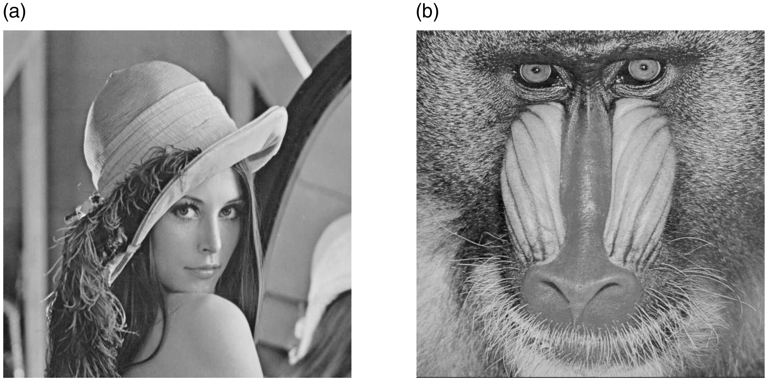
We now consider two test images. These images are the Lena image and Baboon image (see Figure 1). We will apply both Gaussian and impulsive noise to these images. The Gaussian noise has zero mean and variances 0.05 and 0.1, and the salt and pepper noise has densities from 30% through to 80%.

Figure 1.

Lena image (a) and Baboon image (b).

We will now use the three different splines to reconstruct the images. As an example, we will first consider the images corrupted with Gaussian noise with variance 0.05, and impulsive noise of density 60%. In the first image of Figure 2, we show the noisy Lena image. The next three images show the reconstructed images obtained by the three splines. The results for the Baboon image are shown in Figure 3.

Figure 2.

Noisy Lena image ( ${\sigma }^2=0.05$ , 60% salt and pepper noise density) (a), recovered image using gradient penalty spline (b), recovered image using mixed derivative spline (c), recovered image using Laplacian spline (d).

Figure 3.

Noisy Baboon image ( ${\sigma }^2=0.05$ , 60% salt and pepper noise density) (a), recovered image using gradient penalty spline (b), recovered image using mixed derivative spline (c), recovered image using Laplacian spline (d).

We will now show the PSNR for the reconstructed images in Tables 1 to 4.

Table 1.

Lena image PSNR for Gaussian (variance 0.05) and different impulsive noise densities.

	Lena image PSNR
	Noise density
	30%	40%	50%	60%	70%	80%
Grad.	22.13	22.01	22.22	21.90	21.42	20.91
Mixed	22.29	22.28	22.42	21.93	21.59	20.80
Biharm.	22.98	22.95	22.30	22.09	21.74	21.48

Table 2.

Baboon image PSNR for Gaussian (variance 0.05) and different impulsive noise densities.

	Baboon image PSNR
	Noise density
	30%	40%	50%	60%	70%	80%
Grad.	19.14	19.09	18.81	18.48	18.47	18.37
Mixed	19.14	19.08	18.74	18.48	18.35	18.32
Biharm.	18.89	18.71	18.47	18.12	17.84	17.83

Table 3.

Lena image PSNR for Gaussian (variance 0.1) and different impulsive noise densities.

	Lena image PSNR
	Noise density
	30%	40%	50%	60%	70%	80%
Grad.	21.45	21.40	20.81	20.34	20.21	19.82
Mixed	21.77	21.69	20.80	20.44	20.21	19.85
Biharm.	22.20	22.09	21.56	21.10	20.48	20.14

Table 4.

Baboon image PSNR for Gaussian (variance 0.1) and different impulsive noise densities.

	Baboon image PSNR
	Noise density
	30%	40%	50%	60%	70%	80%
Grad.	18.24	18.20	17.93	18.09	17.89	17.65
Mixed	18.18	18.17	17.89	18.06	17.86	17.56
Biharm.	18.06	17.85	17.66	17.54	17.40	17.06

Note that we have chosen our parameter λ using generalised cross validation ¹⁷ and the stochastic trace estimator proposed by Hutchinson. ¹⁸ We note that this gives a good estimate of the optimal parameter. In Figure 4 we have plotted the PSNR and the generalised cross validation function versus λ. Note that the validation function has been scaled for visualisation purposes. For both plots, the Lena image has been corrupted with Gaussian noise with variance 0.05, and has been recovered with the mixed derivative spline. In the left plot, the image has been corrupted with impulsive noise of density 30% while in the right plot the density is 40%.

Figure 4.

Generalised cross validation function and PSNR versus λ for Gaussian noise with variance 0.05 and impulsive noise with densities 30% (a) and 40% (b).

Binary image

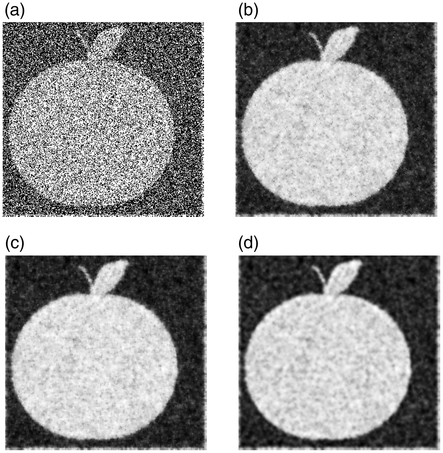
We will now apply the same methods to a binary test image (see Figure 5). As an example, consider the image is corrupted with Gaussian noise of variance 0.05, and impulsive noise of density 60%. We show the noisy image and the reconstructed images in Figure 6.

Figure 5.

Binary image.

Figure 6.

Noisy binary image ( ${\sigma }^2=0.05$ , 60% salt and pepper noise density) (a), recovered image using gradient penalty spline (b), recovered image using mixed derivative spline (c), recovered image using Laplacian spline (d).

We will now show the PSNR for the reconstructed image in Tables 5 and 6.

Table 5.

Binary image PSNR for Gaussian (variance 0.05) and different impulsive noise densities.

	Binary image PSNR
	Noise density
	30%	40%	50%	60%	70%	80%
Grad.	14.77	14.66	14.37	14.19	13.77	13.47
Mixed	15.37	15.21	15.03	14.84	14.43	14.00
Biharm.	15.17	14.93	14.86	14.49	14.39	13.72

Table 6.

Binary image PSNR for Gaussian (variance 0.1) and different impulsive noise densities.

	Binary image PSNR
	Noise density
	30%	40%	50%	60%	70%	80%
Grad.	13.24	13.05	13.01	12.61	12.49	12.20
Mixed	13.58	13.38	13.27	13.03	12.86	12.50
Biharm.	13.36	13.10	12.23	12.88	12.89	12.56

Continuous functions

We would now like to recover continuous functions. We define a tensor product partition ${\mathcal{T}}_h$ of the square $[-1,1]\times [-1,1]$ using the set of points

$$\begin{array}{l}{\mathcal{N}}_h={\left\{(a_i,b_j)\right\}}_{i=1,j=1}^{n,m},\\ \text{where }{a}_i=\frac{2(i-1)}{n-1}-1,\text{and }{b}_j=\frac{2(j-1)}{m-1}-1\end{array}$$

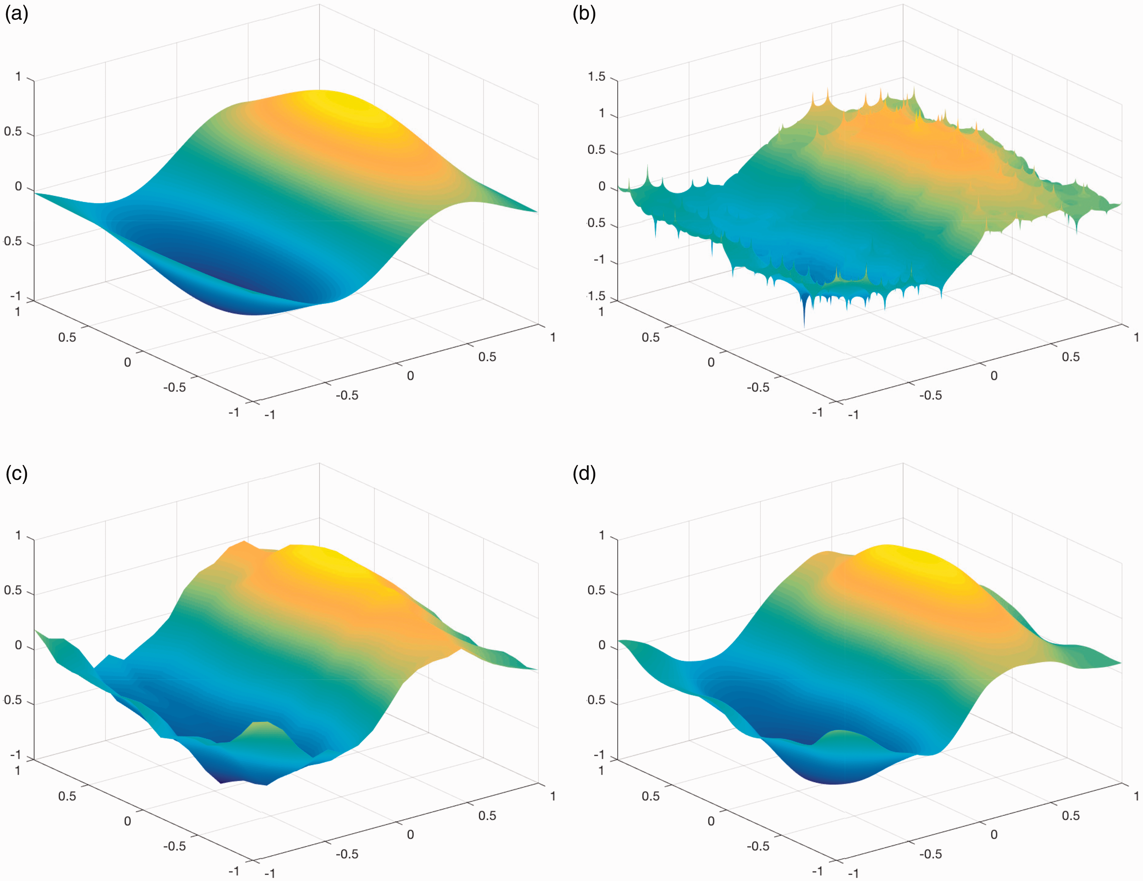
We sample the function value at each point in the partition, and then apply Gaussian noise of variance 0.05. We then refine the partition several times, which halves the mesh size h in each iteration. We will now consider the first test function. Let the function f be given by $f(x,y)=\sin (3x)e^{-x^2-y^2}$ over the domain $[-1,1]\times [-1,1]$ (see Figure 7).

Figure 7.

$f(x,y)=\sin (3x)e^{-x^2-y^2}$ restricted to $[-1,1]\times [-1,1]$ (a), function recovered using gradient penalty spline (b), function recovered using mixed derivative spline (c), function recovered using Laplacian spline (d).

We compare the PSNR values for the recovered function and the original function for different steps of refinement in Table 7, where the refinement step is given by the step-size h.

Table 7.

PSNR for f using different penalty terms.

i	h	Grad.	Mixed	Bihar.
0	2/19	19.85	24.31	25.54
1	1/19	20.01	24.48	26.44
2	1/38	19.59	24.61	26.61
3	1/76	19.16	24.67	26.69
4	1/152	18.51	24.70	26.72
5	1/304	17.95	24.71	26.73

We can see that PSNR values do not increase or decrease for the spline with the mixed derivative penalty and the spline with the Laplacian penalty, whereas the PSNR values decrease for the spline with the gradient penalty. This is due to the fact that the stability constant depends on the mesh-size h for the spline with the gradient penalty.

We show the functions recovered after the fifth iteration in Figure 7. We can see that gradient penalty spline produces a recovered function that overfits the noisy data. On the other hand, both the mixed derivative and the Laplacian splines produce smoother recovered functions.

We want to see the effect of the mesh-size on the spurious spikes of the recovered function. In Figure 8, we show the functions recovered using the gradient penalty spline using the coarser mesh-sizes h = 2/19 and h = 1/19. These pictures show that the spurious spikes are still present although the spikes are slightly smaller in the coarser mesh results.

Figure 8.

Function recovered using gradient penalty spline with h = 2/19 (a), function recovered using gradient penalty spline with h = 1/19 (b).

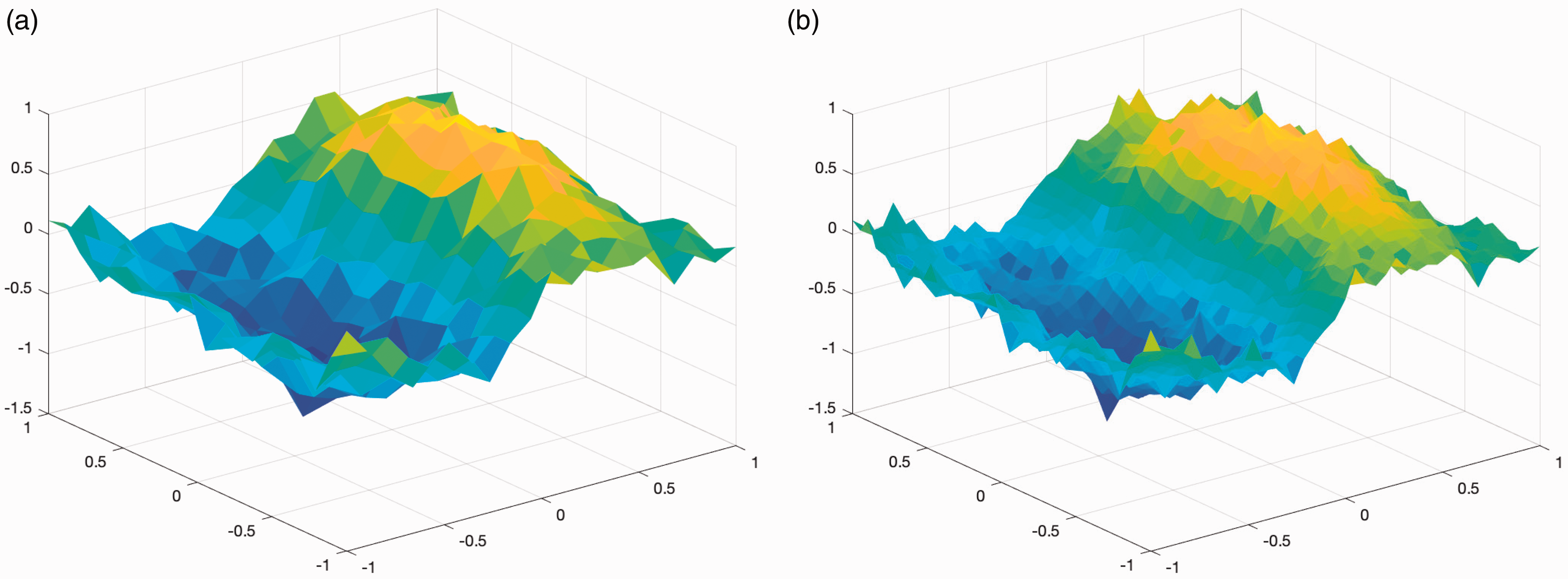
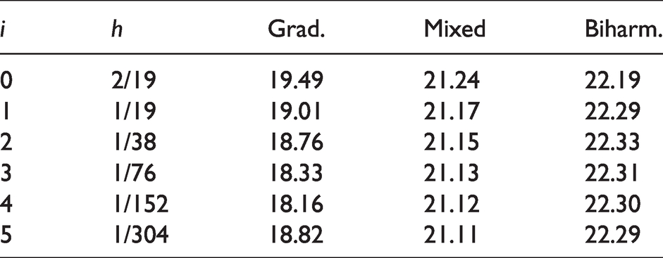
We will now provide a second test function. Let the function g be given by $g(x,y)=-x^2-x{y}^2$ over the domain $[-1,1]\times [-1,1]$ (see Figure 9). We have tabulated the PSNR values for different splines at different levels of refinement in Table 8. The results are similar to the first example but the spurious spikes of the recovered function using the gradient penalty formulation have not affected the PSNR values much in this example.

Figure 9.

$g(x,y)=-x^2-x{y}^2$ restricted to $[-1,1]\times [-1,1]$ (a), function recovered using gradient penalty spline (b), function recovered using mixed derivative spline (c), function recovered using Laplacian spline (d).

Table 8.

PSNR for g using different penalty terms.

i	h	Grad.	Mixed	Biharm.
0	2/19	19.49	21.24	22.19
1	1/19	19.01	21.17	22.29
2	1/38	18.76	21.15	22.33
3	1/76	18.33	21.13	22.31
4	1/152	18.16	21.12	22.30
5	1/304	18.82	21.11	22.29

We show the functions recovered after the fifth iteration in Figure 9. Again, we see that the gradient penalty spline overfits the data.

Discussion

We compared three different bivariate L-spline approaches for removing the mixture of Gaussian and impulsive noise from images. We found that for the Lena image, the Laplacian penalty produced recovered images with the best PSNR. However, we found that the Laplacian penalty performed the worst when recovering the Baboon image. The gradient and mixed derivative penalties performed very similarly to each other when recovering the two real life images. For the Binary image, we found that the mixed derivative penalty performed the best, followed by the Laplacian penalty and then the gradient penalty.

We then applied the same approaches to recover two continuous functions from a set of noisy observations. We found that for both functions, the Laplacian penalty produced the best recovered functions, closely followed by the mixed derivative penalty. The gradient penalty produced recovered functions that overfitted the data.

The overfitting occurred because the gradient penalty formulation is not well-posed in the continuous setting. For dimensions $d\ge 2$ , we have that $H^1(\Omega )\cancel{\subset }{C}^0(\Omega )$ (by the Sobolev embedding theorem). This ill-posedness exhibits itself when the mesh size goes to zero. ¹⁹ The other formulations, however, are well-posed in the continuous setting. This is because $H_m^1(\Omega )\subset C^0(\Omega )$ for any dimension d, ¹⁶ and $H^2(\Omega )\subset C^0(\Omega )$ for dimensions $d\le 3$ .

Overall, the gradient penalty was the simplest spline to implement and the most computationally efficient. However, as this is not well-posed for d > 1, it often produces spurious results. The computational cost of the spline with the mixed derivative penalty is very close to the gradient penalty and this is well-posed for all dimensions. ¹¹ The Laplacian penalty was the least simple to implement, and was the least computationally efficient. Moreover, the spline with the Laplacian penalty is also not well-posed when d > 3. Therefore, we find that the spline with the mixed derivative penalty is the best choice among the presented three splines.