Reducing the residual error of multibeam sounding data through empirical mode decomposition based on cubic Bessel interpolation

Abstract

The systematic residual errors present in multibeam echo-sounding data cause the areas of overlap between adjacent swaths to become distorted. A method is proposed in this paper to reduce the residual error of multibeam sounding data through empirical mode decomposition (EMD) based on cubic Bessel interpolation. Numerical experiments confirm that the discrepancy in the overlap between two swaths is significantly reduced after applying EMD improved by cubic Bessel interpolation compared with both the original water depth data and with data processed using conventional EMD based on cubic spline interpolation. The mean square error of the improved method is decreased by 67% and 29% compared with that of the original and conventional EMD cases, respectively. Therefore, EMD with cubic Bessel interpolation can efficiently reduce the residual error of multibeam echo-sounding data.

Introduction

A multibeam echo sounder, which is a full-coverage sonar system used to acquire depth measurements, is subject to not only its own measurement error but also the influences of external factors, such as sonic velocity changes and positioning, ship attitude and transducer installation deviations.^1–6 At present, researchers are focused primarily on all systematic error sources, the effect of the water column sound speeds, and the bathymetric uncertainties, including the effects of instantaneous attitude and position multibeam and the impacts of transducer installation deviations on the characterization of subsea topography. Various methods have been proposed, including a comprehensive compensation method integrating short-term and long-term heave corrections with combined tidal level and draft corrections, a second-order correction using planar fitting to compensate for transducer installation deviations, and a least squares method-based correction for roll and pitch transducer offsets. These methods have displayed good performance in decreasing the error of multibeam measurements and improving the precision of water depth measurements.^7–11

However, errors inevitably remain in the processed sounding results; these are referred to as residual errors, which cannot be fully eliminated, even with the employment of extremely precise instruments, strict operations, and sophisticated postprocessing schemes. Moreover, the comprehensive effects of residual errors on sounding data can become increasingly significant as the beam depth and incident angle increase with distance, resulting in low-quality sounding measurements; consequently, distortions form in the area of overlap between adjacent bands. ⁹ Unfortunately, it is difficult to accurately estimate the residual errors associated with the processing of sounding data, as they exhibit randomness and obey a Gaussian distribution. In this context, the empirical mode decomposition (EMD) method can effectively resolve this issue. EMD generally begins by decomposing multibeam sounding data in one dimension and then constructing trend and residual terms for the sounding data to establish the overall data trend term using the central beam trend; the subsea topography is finally restored by adding the residual term of the sounding data.

However, in the decomposition process, the original EMD technique adopts cubic spline interpolation to obtain the upper and lower envelopes of the original data, often leading to extrema, such as those related to overshoot and undershoot issues. The overshoot or undershoot of the envelope curve refers to the “peak” or “valley” between two adjacent extreme points during the envelope fitting process. As a result, the envelope curve fails to completely envelop the change in the signal shape, which leads to errors in EMD. In addition, endpoint drift occurs, leading to the inward propagation of the endpoint error and the introduction of false modal components, thereby leading to a reduction in the final residual error.^12–15 To overcome these problems, Mao et al. ¹⁶ proposed the use of piecewise power function interpolation to reduce the influence of the extreme phenomenon of the envelope curve. Cai et al. ¹⁷ proposed a local integral average-constraint cubic spline interpolation algorithm to improve the cubic spline interpolation in the original EMD algorithm. Huang et al. ¹⁸ proposed the use of a mirror extension method to eliminate the effect of endpoint drift. Wu and Sherman et al. ¹⁹ proposed a boundary extension to improve the phenomenon of endpoint migration. Thus, EMD has been widely used in various academic areas due to its distinct advantages; however, it also needs to be further improved because of some shortcomings. ²⁰

In this paper, a method is proposed to reduce the residual error of multibeam sounding data using Bessel interpolation-based EMD on the basis of cubic spline interpolation-based EMD. By matching the common ping sections of adjacent swaths using Bessel interpolation, EMD, and a trend term difference calculation, the proposed method performs satisfactorily in reducing the residual errors of multibeam sounding data.

Materials and methods

Principle of EMD

In essence, EMD involves the smoothing of nonstationary signals; the core concept of this method is consistent with that of Fourier transform and wavelet transform insomuch that signals are decomposed in a stepwise manner into a set of intrinsic mode functions (IMFs). Nevertheless, EMD differs from these two methods insomuch that it smooths the signal according to the time scale characteristics of the signal without the need to establish base functions. The implementation of EMD involves the determination of the difference between the original signal and the average values of the upper and lower envelopes. If a difference value satisfies the conditions of the IMF, it is defined as the first IMF. Then, the decomposition process proceeds with the rest of the series until the stop condition for decomposition is met.^{14,18,21–26}

An IMF should satisfy the following two conditions^27–29

Throughout the whole series, the number of extreme points should not differ by more than 1 from the number of zero-crossing points.

At any point, the average values of the upper envelope determined by the local maximum value of the signal and the lower envelope determined by the local minimum value of the signal should be zero.

The filtering criterion is as follows^22,30

$$SD={\displaystyle \sum \left|\frac{h_{1,\left(k-1\right)}(t)-h_{1,k}(t)}{h_{1,k}^2(t)}\right|}$$

(1)

where $h_{1,\left(k-1\right)}\left(t\right)$ is the result of the $\left(k-1\right)$ -th screening, and j is the result of the k-th screening. The stop criterion is satisfied when the last intrinsic mode component or the remaining intrinsic mode component is less than a prescribed value. Under this condition, no IMF can be further decomposed, and the iteration process is terminated. The flowchart is shown in Figure 1.

Figure 1.

Flowchart of cubic Bessel interpolation-based EMD.

During the application of EMD to the original data, due to the lack of extreme points at the two endpoints of the signal, endpoint divergence may occur when cubic spline interpolation is used to fit the envelope. This problem deteriorates the decomposition quality but can be suppressed by using the mirror extension method for the endpoints.

Cubic polynomial Bessel interpolation

To overcome the disadvantages of cubic spline interpolation in its application in EMD, this paper introduces a piecewise cubic polynomial Bessel interpolation algorithm to fit both the upper and lower envelopes and the mean value curve.

It is assumed that the data sequence of a signal is $\mathrm{g}\left({\tau }_1\right),\cdots \cdots ,\mathrm{g}\left({\tau }_n\right)$ with $\mathrm{a}={\tau }_1<\cdots <{\tau }_n=b$ . A series of piecewise cubic interpolation functions $\mathrm{f}$ can be constructed for the sequence $\mathrm{g}$ . In each interval $[{\tau }_i,\cdots {\tau }_{i+1}]$ , the order of the interpolation function $P_i$ for $\mathrm{f}$ should be four: ³¹

$$f\left(x\right)=P_i\left(x\right)$$

(2)

where ${\tau }_i\le x\le {\tau }_{i+1}$ , $P_i\in \Pi <4,\mathrm{and}\mathrm{ }i=1,\cdots ,n-1$ .

For the $i$ -th segment, the fitting interpolation function $P_i$ should satisfy the following conditions:

$$P_i\left({\tau }_i\right)=\mathrm{g}\left({\tau }_i\right)P_i\left({\tau }_{i+1}\right)=g\left({\tau }_{i+1}\right) {P^{\mathrm{\prime }}}_i\left({\tau }_i\right)=s_i\mathrm{ }{P^{\mathrm{\prime }}}_i\left({\tau }_{i+1}\right)=s_{i+1}(\mathrm{ }i=1,\cdots ,n-1)$$

(3)

where $s_1,\cdots ,s_n$ are free factors.

The ultimate piecewise cubic interpolation function $\mathrm{f}$ should be the same as $\mathrm{g}$ in the intervals of ${\tau }_1,\cdots ,{\tau }_n$ and $[a,b]$ . This paper adopts the Newton interpolation formula to calculate the polynomial coefficients for the $\mathrm{i}$ -th piecewise interpolation function $P_i$ :

$$P_i\left(x\right)=P_i\left({\tau }_i\right)+\left(x-{\tau }_i\right)\left[{\tau }_i,{\tau }_i\right]P_i+{\left(x-{\tau }_i\right)}^2\left[{\tau }_i,{\tau }_i,{\tau }_{i+1}\right]P_i+{\left(x-{\tau }_i\right)}^2\mathrm{ }(x-{\tau }_{i+1})\left[{\tau }_i,{\tau }_i,{\tau }_{i+1},{\tau }_{i+1}\right]P_i$$

(4)

where $\left[{\tau }_i,{\tau }_i\right]P_i$ is the first-order divided difference of $P_i$ at ${\tau }_i,{\tau }_i$ , $\left[{\tau }_i,{\tau }_i,{\tau }_{i+1}\right]P_i$ is the second-order divided difference of $P_i$ at ${\tau }_i,{\tau }_i,{\tau }_{i+1}$ and $\left[{\tau }_i,{\tau }_i,{\tau }_{i+1},{\tau }_{i+1}\right]P_i$ is the third-order divided difference of $P_i$ at ${\tau }_i,{\tau }_i,{\tau }_{i+1},{\tau }_{i+1}$ . We determine these differences from the divided difference table for $P_i$ , as shown in Table 1.

Then, the above formula can be converted into the following form in terms of the shifted powers ${(x-{\tau }_i)}^r$ .

$$P_i\left(x\right)=c_{1,i}+c_{2,i}\left(x-{\tau }_i\right)+{c_{3,i}(x-{\tau }_i)}^2+c_{4,i}{\left(x-{\tau }_i\right)}^3$$

(5)

From the above equation, one can obtain the following equation set:

$$c_{1,i}=P_i\left({\tau }_i\right)=g\left({\tau }_i\right)$$

$$c_{2,i}={P\mathrm{\prime }}_i\left({\tau }_i\right)=s_i$$

$$c_{3,i}=\frac{{P^{\mathrm{\prime }\mathrm{\prime }}}_i\left({\tau }_i\right)}{2}=\left[{\tau }_i,{\tau }_i,{\tau }_{i+1}\right]P_i-\Delta {\tau }_i\left(\left[{\tau }_i,{\tau }_i,{\tau }_{i+1},{\tau }_{i+1}\right]P_i\right)=\frac{\left[{\tau }_i,{\tau }_{i+1}\right]g-s_i}{\Delta {\tau }_i}-c_{4,i}\Delta {\tau }_i$$

$$c_{4,i}=\frac{{P^{\mathrm{\prime }\mathrm{\prime }\mathrm{\prime }}}_i\left({\tau }_i\right)}{6}={(s}_i+s_{i+1}-2[{\tau }_i,{\tau }_{i+1}]\mathrm{g})/{(\Delta {\tau }_i)}^2$$

(6)

The slope $s_i$ should be numerically equal to the slope of the cubic polynomial $P$ at time ${\tau }_i$ ; this slope is the same as that of $g$ at times ${\tau }_{i-1},{\tau }_i$ , and ${\tau }_{i+1}$ . Then, the piecewise cubic polynomial Bessel interpolation formula can be simplified as:

$$s_i=\frac{\Delta {\tau }_i\left[{\tau }_{i-1},{\tau }_i\right]\mathrm{g}+\Delta {\tau }_{i-1}[{\tau }_1,{\tau }_{i+1}]g}{\Delta {\tau }_i+\Delta {\tau }_{i+1}}$$

(7)

The use of the Bessel interpolation results as data points to fit the curve improves the fitting accuracy for the upper and lower envelopes as well as the mean value curve, and thus, more reliable IMFs are obtained.

Reducing the errors of multibeam sounding data by Bessel interpolation-based EMD

The main steps in processing multibeam data using cubic Bessel interpolation-based EMD to reduce the residual errors are as follows.

Identification of the common ping section of adjacent swaths

The common ping sections of adjacent swaths can be identified by either the minimum distance method or the minimum deflection angle method. When using the minimum distance method, the lowest point of a swath is taken as the reference point, and then find the lowest point with the shortest straight-line distance from the reference point among all adjacent swaths. The pings where the identified points are located are regarded as the common ping section of adjacent swaths. However, this method is not applicable to the case in which the ping is lost in the sounding data. In this context, the minimum deflection angle method can be employed to match the common ping sections of adjacent swaths. Specifically, when the trajectory is a straight line, the straight line connecting the lowest points in the ping sections of the swaths to the left and right should be orthogonal to the survey line, and the deflection angle should be 0. When the trajectory is not a straight line, we need to find a lowest point in the right swath, which is closest to the lowest point in the left reference swath. And it is necessary to make sure that the connecting line between the two points and the orthogonal line of the trajectory have the smallest deflection angle. In this case, given the small distance from the lowest point to the orthogonal point in the right swath, the corresponding ping section should be able to reflect the true topographic variations between swaths.

EMD processing of original data

The cubic spline interpolation-based EMD technique is used to decompose the water depth data for the common ping sections of adjacent swaths $H_1\left(t\right)$ and $H_2\left(t\right)$ into the subsea trend terms $R_1$ and $R_2$ and the residual terms $h_1\left(t\right)$ and $h_2\left(t\right)$ .

Cubic Bessel interpolation

Cubic Bessel interpolation is used to interpolate the extreme points, as shown in Figure 1.

The specific steps in this interpolation process are as follows.

(1) Filtering of extreme points

The maximum and minimum points are filtered and removed from the original water depth data. Moreover, the mirror extension method is applied to the extreme points; consequently, the maximum and minimum values are extended for the two extreme points at the two endpoints. The extended extreme point data are used as the sample points for cubic Bessel interpolation.

(2) Selection of control points for cubic Bessel interpolation

To perform cubic Bessel interpolation, two control points are selected between each set of two extreme points. The following formulas are selected by the algorithm:

$${\mathrm{A}}_{\mathrm{i}}({\mathrm{x}}_{\mathrm{i}}+\mathrm{a}\left({\mathrm{x}}_{\mathrm{i}+1}-{\mathrm{x}}_{\mathrm{i}-1}\right),{\mathrm{y}}_{\mathrm{i}}+\mathrm{a}({\mathrm{y}}_{\mathrm{i}+1}-{\mathrm{y}}_{\mathrm{i}-1}\left)\right)$$

$${\mathrm{B}}_{\mathrm{i}}({\mathrm{x}}_{\mathrm{i}+1}-\mathrm{b}\left({\mathrm{x}}_{\mathrm{i}+2}-{\mathrm{x}}_{\mathrm{i}}\right),{\mathrm{y}}_{\mathrm{i}+1}-\mathrm{b}({\mathrm{y}}_{\mathrm{i}+2}-{\mathrm{y}}_{\mathrm{i}}\left)\right)$$

(8)

where $A_i$ and $B_i$ are the first and second control points, respectively, between the $\mathrm{i}$ -th point and the $(\mathrm{i}\mathrm{ }+\mathrm{ }1$ )-th point; $x$ and $y$ are the coordinates of a control point; and $\mathrm{a}$ and $\mathrm{b}$ are the corresponding coefficients that reflect the quality of the selected control point. Based on multiple tests, $\mathrm{a}\mathrm{ }=\mathrm{ }\mathrm{b}\mathrm{ }=\mathrm{ }1/12$ was empirically obtained. The effect of selecting control points is shown in Figure 2.

Figure 2.

Effect of control point selection.

In Figure 2, the solid line represents a part of the original data that was removed, the symbol “o” represents the minimum value point extracted from the original data, and the symbol “*” represents a control point; notably, the control points were calculated according to formula (8). Based on Figure 2, two control points are added between every two adjacent minimum points according to the above formula. In the next step, it is necessary to draw the lower envelope curve based on these control points and the minimum points. The maximum points and the control points of the upper envelope curve are selected in the same way.

(3) Cubic Bessel interpolation

After selecting the control points, cubic Bessel interpolation is performed using the selected control and sample points.

The Bessel interpolation formula is expressed as:

$$x=P_{x1}{(1-t)}^3+3P_{x2}t{\left(1-t\right)}^2+3P_{x3}{t}^2(1-t)+P_{x4}{t}^3$$

$$y=P_{y1}{(1-t)}^3+3P_{y2}t{(1-t)}^2+3P_{y3}{t}^2\left(1-t\right)+P_{y4}{t}^3$$

(9)

This representation is basically cubic Bessel interpolation in parametric form, where ( $P_{x1}$ , $P_{y1}$ ) and ( $P_{x4}$ , $P_{y4}$ ) are the coordinates of two adjacent extreme points; ( $P_{x2}$ , $P_{y2}$ ) and ( $P_{x3}$ , $P_{y3}$ ) are the coordinates of two control points between adjacent extreme points that are determined by formula (8); and t is a parameter related to the smoothness of the Bessel curve. The lower envelope curve drawn according to the extreme points and control points obtained in step (2) is shown in Figure 3, and it is obtained using the cubic Bessel interpolation method shown in formula (9).

Figure 3.

Effect of the lower envelope curve.

As shown in Figure 3, the solid line is a portion of the original data, the dotted line is the lower envelope curve drawn according to the cubic Bessel interpolation method, and the upper envelope curve is drawn in the same way as the lower curve.

(4) EMD processing using cubic Bessel interpolation.

The cubic spline interpolation technique in the original EMD method is replaced by the abovementioned cubic Bessel interpolation approach, which is used to obtain the decomposition results.

(5) Calculation of the difference between the trend terms of the fitting curves for the central beam and edge beam.

The trend terms $R_1$ and $R_2$ of the central beam of the common ping section are fitted, and the fitting curve replaces the trend term L of the edge beam. Quadratic curve fitting is conducted for the central beam, and the difference between the simulated fitting curve of the central beam and the trend term of the edge beam forms the trend term $L^{\mathrm{\prime }}$ of the edge beam.

(6) Construction of the trend term $\mathrm{R}=C_1+C_2+L^{\mathrm{\prime }}$ of subsea topography.

This term is added to the residual term to restore the subsea topography.

Results

Following the above steps, the multibeam bathymetric data of two swaths are subjected to EMD. The trend term and residual term of the water depth data are constructed according to the relationship between the water depth data and the decomposed IMF. The detailed procedure is summarized as follows.

(1) Search all the maximum and minimum points of the water depth data H(t) for each ping. Additionally, use cubic Bessel interpolation to fit the upper envelope and the lower envelope , and calculate the average .

(2) Subtract the average from the original data H(t) to obtain the class distance average a(t). Determine if a(t) satisfies the conditions for the IMF. If the conditions are satisfied, a(t) is the first decomposed mode component; if not, regard a(t) as the original data, and repeat the operation in equation (1) until the IMF conditions are met.

(3) Remove the first mode component from the original data, and repeat equation (1) and (2) for mode decomposition until the IMF conditions are met, finally resulting in three IMFs and one trend term, as shown in Figure 4.

Figure 4.

Water depth and EMD results for a single ping. (a) Water depth data from a single ping, (b) IMF1, (c) IMF2, (d) IMF3, (e) IMF4 and (f) IMF5, (g) IMF6, (h) IMF7 and (i) trend term.

The water depth of a certain single-ping section is shown in Figure 4(a), and the intrinsic mode components after the application of EMD are illustrated in Figure 4(b) to (h). The trend term after decomposition is presented in Figure 4(i). The intrinsic mode components after EMD, each corresponding to water depth data at a specific frequency, are arranged with respect to the scale.

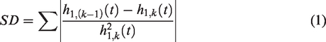
The influence of residual error on sounding data is mainly in the edge beam and the long wave term after decomposition, ³² therefore, the water depths of edge beam is corrected in this paper. Figure 5 includes the semi-central beam and the edge beam for the adjacent swaths. The ping sections corresponding to two selected survey lines are shown in Figure 5(a), in which the solid line represents the water depth of the ping section of the left swath and the dashed line represents that of the right swath. The application of EMD to the water depth data corresponding to the ping sections of the two swaths results in two sets of intrinsic mode components and a trend term R. Then, the trend term and residual term of the water depth data corresponding to the two swaths are constructed, as shown in Figure 5(b) and (c). The central beam is intercepted by the water depth trend terms of the two swaths, the variation in the water depth trend term of the central beam is fitted using a quadratic curve, and the pattern of the variation in the edge beam is simulated. Thus, the edge beam in the original trend term is replaced, as shown in Figure 5(d), where the dashed line represents the replaced trend term of the edge beam.

Figure 5.

Reducing the residual error associated with water depth data for two swaths. (a) Water depth in a common ping section, (b) trend terms of the ping sections of the two swaths, (c) residual terms of adjacent ping sections, (d) edge beam trend term simulated, (e) comparison between the simulated and original trend terms, (f) water depth of the two swaths after.

The water depth data are restored by summing the reconstructed overall water depth trend term and the overall residual term, as shown in Figure 5(f). A comparison between the restored and original water depth data for the single-ping section clearly demonstrates that the residual error has been effectively reduced.

(4) The aforementioned shortest distance method is used to search the corresponding ping sections; then, the survey line data for adjacent swaths are extracted. The water depth data for each ping section are processed following steps (1) through (3). An overall reduction in the residual error of the two swaths can be achieved by repeating the process for each ping, and the residual error of multibeam sounding data can be reduced. Taking multibeam sounding terrain data with an incident angle of 0 to 35° as an example, the residual error is suppressed, and a comparison of the terrain before and after residual error reduction is presented in Figure 6.

Figure 6.

Topographic maps before and after residual error reduction. (a) Topographic map before residual error reduction and (b) topographic map after residual error reduction.

A comparison between Figure 5(f) and (a) shows that the residual error of the multibeam sounding data is effectively reduced. Moreover, Figure 6 is the DEM of the water depths, which contains the half-central beam and the edge beam of the two adjacent trajectories. In Figure 6(a), the obvious “bumps” of the overlap of edge beam can be seen in the DEM of original water depths, after the residual error reduction, in Figure 6(b), the obvious “bumps” have been eliminated, and some “sags” have been improved to a certain extent. The DEM on both sides of the half-central beam retains its original appearance. These findings validate the effectiveness of the proposed method.

To quantitatively compare and analyze the performance of the residual error reduction, the results of cubic spline interpolation-based EMD are compared with the results using the method proposed in this paper, as shown in Table 2.

Table 1.

Divided difference table for $P_i$ .

	[ ] P	[ , ] P	[ , ,] P	[ , , ,] P
${\tau }_i$	$g\left({\tau }_i\right)$
		$s_i$
${\tau }_i$	$g\left({\tau }_i\right)$		$\frac{\left[{\tau }_i,{\tau }_{i+1}\right]g-s_i}{\Delta {\tau }_i}$
		$\left[{\tau }_i,{\tau }_{i+1}\right]g$		$\frac{{(s}_i+s_{i+1}-2[{\tau }_i,{\tau }_{i+1}]\mathrm{g})}{{(\Delta {\tau }_i)}^2}$
${\tau }_{i+1}$	$g\left({\tau }_{i+1}\right)$		$\frac{s_{i+1}-\left[{\tau }_i,{\tau }_{i+1}\right]g}{\Delta {\tau }_i}$
		$s_{i+1}$
${\tau }_{i+1}$	$g\left({\tau }_{i+1}\right)$

Table 2.

Discrepancy between adjacent swaths.

Statistic	Water depth discrepancy/m	Average/m	Mean square error/m
Original water depth	–0.094–0.143	0.072	0.036
Water depth based on cubic spline interpolation-based EMD	–0.065–0.033	0.022	0.017
Water depth based on cubic Bessel interpolation-based EMD	–0.050–0.034	0.021	0.012

The overlapping area has an average water depth of -23.38 m in this region. According to the water transport measurement specification, the depth difference in an overlapping area should not exceed 2% of the water depth, that is, 0.47 m. The maximum absolute value of the original water depth discrepancy in this area is 0.143 m, which is smaller than 0.47 m; thus, the requirement of the water transport measurement specification is met. Table 2 demonstrates that the mean square error in the case of cubic spline interpolation-based EMD is approximately 0.02 m less than that of the original method, indicating that cubic spline interpolation-based EMD can, to some extent, reduce the residual error of multibeam sounding data. For the improved cubic Bessel interpolation-based EMD method, the discrepancy in the overlap between two swaths is apparently less than the discrepancies in both the original data and the data processed using cubic spline interpolation-based EMD; moreover, the average is the lowest using the proposed method, and the mean square error is decreased by 67% and 29% compared with that of the original data and the data processed using cubic spline interpolation-based EMD, respectively. Therefore, the cubic Bessel interpolation-based EMD technique is able to efficiently reduce the residual error in multibeam sounding data.

Discussion

In Table 2, the same set of original data is used for the three experimental control methods, and the water depth discrepancies of the three methods are inconsistent. The reasons for the inconsistencies are as follows.

First, the original water depth is collected by direct measurement. Because there is no processing, the range of the water depth discrepancy in the overlapping coverage area of adjacent ping sections is relatively large, and the corresponding mean square error is also large.

The second method, the EMD method based on cubic spline interpolation, calculates the water depth discrepancy value, which is the discrepancy of the water depth in the common coverage area of adjacent ping sections after the residual error of the original EMD method has been reduced. This value is compared with the original value. The range of water depth discrepancies is reduced to some extent with this approach, and the corresponding mean square error is also reduced.

The third method, the EMD method based on cubic Bessel interpolation used in this paper, yields a significant reduction in the water depth discrepancy of the common coverage area of adjacent ping sections after processing. The mean square error is close to zero, which reflects the effectiveness of the method proposed in this paper to a certain extent.

The proposed Bessel interpolation-based EMD method decreases, to some degree, the residual error of multibeam sounding data. ¹³ It should be noted that the selection of the incident angle of the central beam has a certain effect on the fitting of the trend term of the edge beam, which will further influence the performance of residual error reduction. ³³ However, in engineering practice, it is difficult to accurately determine the central beam considering various subsea topographies. For this reason, in this study, the residual error of the corresponding ping section is reduced with different central beam incident angles at an increment of 5°; the corresponding results are given in Table 3.

Table 3.

Discrepancy between corresponding ping sections at various central beam incident angles.

Incident angle of the central beam/°	Statistic	Water depth discrepancy/m	Average/m	Mean square error/m
0–5	Original water depth	–0.122–0.134	0.064	0.036
	Water depth based on cubic spline interpolation-based EMD	–0.082– 0.018	0.027	0.024
	Water depth based on cubic Bessel interpolation-based EMD	–0.070–0.027	0.022	0.019
0–10	Original water depth	–0.122–0.134	0.064	0.036
	Water depth based on cubic spline interpolation-based EMD	–0.082–0.018	0.027	0.024
	Water depth based on cubic Bessel interpolation-based EMD	–0.071–0.026	0.023	0.019
0–15	Original water depth	–0.122–0.134	0.064	0.036
	Water depth based on cubic spline interpolation-based EMD	–0.083–0.018	0.027	0.024
	Water depth based on cubic Bessel interpolation-based EMD	–0.071–0.025	0.023	0.020
0–20	Original water depth	–0.122–0.134	0.064	0.036
	Water depth based on cubic spline interpolation-based EMD	–0.082–0.018	0.028	0.024
	Water depth based on cubic Bessel interpolation-based EMD	0.071–0.025	0.023	0.020
0–25	Original water depth	–0.122–0.134	0.064	0.036
	Water depth based on cubic spline interpolation-based EMD	–0.081–0.018	0.026	0.023
	Water depth based on cubic Bessel interpolation-based EMD	–0.070–0.026	0.022	0.019
0–30	Original water depth	–0.122–0.134	0.064	0.036
	Water depth based on cubic spline interpolation-based EMD	–0.081–0.018	0.026	0.023
	Water depth based on cubic Bessel interpolation-based EMD	–0.068–0.028	0.022	0.018
0–35	Original water depth	–0.122–0.134	0.064	0.036
	Water depth based on cubic spline interpolation-based EMD	–0.079–0.020	0.025	0.022
	Water depth based on cubic Bessel interpolation-based EMD	–0.066–0.031	0.021	0.017
0–40	Original water depth	–0.122–0.134	0.064	0.036
	Water depth based on cubic spline interpolation-based EMD	–0.078–0.021	0.025	0.023
	Water depth based on cubic Bessel interpolation-based EMD	–0.063–0.033	0.021	0.018

The overlapping area in Table 3 has an average water depth of -23.41 m, and the maximum absolute value of the original water depth discrepancy is 0.134 m, which is smaller than 0.46 em, the value required in the water transport measurement specification. Table 3 clearly shows that the water depth discrepancy and average value both change slightly in the applications of both cubic spline interpolation and cubic Bessel interpolation-based EMD with variations in the incident angle of the central beam. After residual error reduction using the central beams corresponding to different central beam incident angles, the water depth discrepancy range obtained by using the EMD method based on cubic Bessel interpolation proposed in this study is far smaller than the original water depth discrepancies at different incidence angles and slightly smaller than that obtained by using EMD based on cubic spline interpolation. Therefore, the method proposed in this study yields an overlapping area with a smaller water depth variation than that obtained by other methods. Moreover, the mean square error of the water depth data processed by the EMD method based on cubic Bessel interpolation is 50% smaller on average than that of the original water depth data and 20% smaller on average than that obtained with the EMD method based on cubic spline interpolation. Specifically, the mean square error is suppressed the most at an incident angle of 0 to 35°, reaching 23%, and it is suppressed the least at an incident angle of 0 to 15 at only 17%.

The water depth discrepancy will affect the splicing effect of adjacent ping sections. For example, in Table 2, the original water depth data have the worst splicing effect for adjacent ping sections, and there is obvious “crossing” due to the large range of discrepancies. After the residual error is reduced by the EMD method based on cubic Bessel interpolation, the splicing effect of adjacent ping sections is improved because the range of water depth discrepancies is significantly reduced.

For an intuitive comparison of the mean square residual errors corresponding to the cubic spline interpolation-based EMD and cubic Bessel interpolation-based EMD methods, the mean square errors of the discrepancies between two adjacent swaths at different central beam incident angles are plotted in Figure 7.

Figure 7.

Mean square error of the adjacent bands of water depth discrepancies at different central beam incident angles.

As shown in Figure 7, the selection of the central beam incident angle has a clear influence on the residual error reduction. Moreover, the mean square error of the water depth discrepancy of the data processed by the traditional EMD method based on cubic spline interpolation is significantly smaller than that of the original, non-processed data. Moreover, the mean square error of the water depth data processed with the EMD method proposed in this study is not only significantly smaller than that of the original, non-processed data but also smaller than that of the data processed by the traditional EMD method. Therefore, it is safe to conclude that the EMD method based on the cubic Bessel interpolation contributes to the best residual error reduction.

To evaluate the data fitting performance, the goodness of fit is calculated, which is usually expressed by R2:

R^2 = ESS/TSS (10)

where ESS is the explained sum of squares and TSS is the total sum of squares. Theoretically, the closer R2 is to 1, the higher the quality of the fit. The goodness of fit of the central beam incidence angle of the experimental data is shown in Table 4.

Table 4.

Goodness of fit for different central beam angles.

Incident angle of the central beam/°	R2
0–5	0.9759
0–10	0.9636
0–15	0.9332
0–20	0.9349
0–25	0.9475
0–30	0.9503
0–35	0.9982
0–40	0.9781

As shown in Table 4, incident angles in the range of 0 to 35° contribute to the highest R2, which is close to 1, whereas incident angles in the range of 0 to 15° result in the lowest R2, which is far from 1. Therefore, the data fitting performance is the best when the incident angle is in the range of 0 to 35°. This result is consistent with the above argument that a central beam with an incident angle in the range of 0 to 35° leads to the lowest mean square error after the residual error reduction.

Conclusions

This paper introduces Bessel interpolation into EMD and proposes an approach to reduce the residual error of multibeam sounding data using cubic Bessel interpolation-based EMD. A comparison of the discrepancies between adjacent swaths, averages, and mean square errors resulting from the proposed and conventional EMD methods indicates that the proposed EMD technique can, to a large extent, reduce the residual error of multibeam sounding data. In reducing the residual error of multibeam sounding data for different terrain types, the proposed method yields a small average water depth discrepancy, and the mean square error is reduced by 67% and 29%, respectively, when compared with the values based on the original data and the data processed by the traditional EMD method.

At different central beam incident angles, the performance of the method proposed in this paper to reduce the residual error of multibeam sounding data varies. Therefore, future studies should focus on investigating the suitability of the proposed method for different subsea topographies. Moreover, the results of this study are influenced by the selection of the corresponding coefficients and the data fitting method used for the control points of the Bessel curve. Future research could focus on how to adaptively determine the corresponding coefficients and choose an optimal data fitting method.