Selective segmentation of a feature that has two distinct intensities

Abstract

It is common for a segmentation model to compute and locate edges or regions separated by edges according to a certain distribution of intensity. However such edge information is not always useful to extract an object or feature that has two distinct intensities e.g. segmentation of a building with signages in front or of an organ that has diseased regions, unless some of kind of manual editing is applied or a learning idea is used. This paper proposes an automatic and selective segmentation model that can segment a feature that has two distinct intensities by a single click. A patch like idea is employed to design our two stage model, given only one geometric marker to indicate the location of the inside region. The difficult case where the inside region is leaning towards the boundary of the interested feature is investigated with recommendations given and reliability tested. The model is mainly presented 2D but it can be easily generalised to 3D. We have implemented the model for segmenting both 2D and 3D images.

Introduction

Segmentation of an image is the task of partitioning it into different segments in order to classify and identify objects. Although often the concepts of segmentation and feature extraction are synonymously used, they are not always the same thing. This paper considers a common setting where an interested object or feature has two distinct intensities e.g. segmentation of a building with signages in front or of an organ that has diseased regions. Here the segmented results by the common models show parts of an object, or not a complete object. In particular we consider this challenging setting and assume both domains have distinct intensities and are approximately homogeneous, so that a region based model is applicable.

Classic variational approaches such as the Mumford and Shah ¹ method aims to partition the entire image domain . Here n regions such that $\Omega ={\Omega }_1\cup {\Omega }_2\cup \dots \cup {\Omega }_n$ by finding an edge ition the entire image domain . Here the segmented results by the common models show parts of an object, or nots in an image, however it is difficult to accurately solve. Chan and Vese ² introduced a piecewise constant version of the Mumford-Shah model, overcoming the difficulty of solving Mumford-Shah model; another approach is by Ambrosio and Tortorelli, ³ who proposed an approximation to Mumford-Shah using t\\Normalization\\IN\\INPROCESS\\1“ \o ”1=Ref L. Ambrosioand V.variational segmentation models for global segmentation i.e. locating all edges and different regions. Another common type are known as edge based, which aim to evolve a contour towards edges in an image by making use of an edge detector. Kass et al. ⁴ was among the first of this type, which was further developed by the Geodesic Active Contours model by Caselles et al. ⁵

Selective segmentation aims to identify a particular object or objects of interest, and so has very important applications in medical imaging. A set $\mathcal{M}$ of marker points (usually 3to identify a particular object or objects of interest, and so has very important applications et al., ⁶ who introduced a distance constraint to the GAC model. A popular method to achieve selective segmentation is to combine elements from both region based and edge based models, as was done in Badshah and Chen ⁷ to encourage the contour to fit to the intensity of an object. Rada and Chen ⁸ made this more reliable by adding a constraint on the evolution of the contour by making use of the polygon formed by the marker points. More recently, Spencer and Chen ⁹ introduced a convex model making use of the Euclidean distance from the set of marker points as a constraint. This model is able to achieve good results, however can be parameter sensitive and not as robust. It is recently improved in Roberts et al. ¹⁰ by replacing the Euclidean distance with a Geodesic distance, which increases distance in an image when an edge is detected and only needs a single marker point. For selective segmentation, this is the most robust model discussed so far and is the model which we will use to obtain our segmentation results. To illustrate the differences, we refer to Figure 1 where the purpose is to segment the aorta in a real life CT image with a stent (stance in an image when an edge is detected and only needs a single marker point. For selective segmentation, this is the

Figure 1.

Illustration of the performance of an old model Roberts et al. ¹⁰ in (a)–(j): its dependence on the initial marker set l Roberts8" in microscopic images as a prelude to development of computer assisted automated di–(o), to segment the complete object in (n). (a) Marker set 1. (b) Marker set 2. (c) Marker set 3. (d) Marker set 4. (e) Marker set 5. (f) Result 1. (g) Result 2. (h) Result 3. (i) Result 4. (j) Result 5. (k) Marker set. (l) Stage 1. (m) Stage 2. (n) Final. (o) Combined.

However this paper addresses the case where the intended object has inhomogeneous intensities that may be broadly grouped into two regions of pixels each having a very different mean-intensity value. Then none of the above mentioned existing models can be used because there exist xist r this pes’ in the object that we are interested in.

To be precise, the task is to take a single input from the user to obtain segmentations of two separate, connected objects: one for the object with a marker, and the other for a larger object containing the first. In this paper we propose a nobel and yet simple method for this task. The class of the secondary objects that we can segment contains typically two phases in terms of intensities. Such an object cannot be segmented by all the known methods without manual editing. It is possible that a learning model can do the same job but such a model can deal with one type of applications per training, not for the variety of applications that we aim for.

We begin by detailing the segmentation model and then discuss some natural approaches to find a value to threshold our image in order to segment it a second time, before introducing our idea of thresholding an image in order to model the three-phase segmentation using a two-phase model. Finally, we discuss where the method might fail and then recommend a solution.

The previous segmentation works

Let z(x, y) be a given image defined on the image domain $\Omega \subset {ℝ}^2$ . The task of selective segmentation is to segment the object in image z that is closest to an user-provided set $\mathcal{M}=\{(x_i,y_i)\in \Omega \}$ . However the new task that this paper tries to address is the case where the intended object has inhomogeneous intensities that may be broadly grouped into two regions of pixels each having a very different mean-intensity value. Then it is not immediately obvious which existing models can be used e.g. either Mumford-Shah type or edge type models cannot be used because there exist xist ver the new task that this paper tries to address is the case where the intende representative models that we use to build our new models.

A two-phase model

We denote ${\Omega }_1$ as the foreground object, and ${\Omega }_2=\Omega \backslash {\Omega }_1$ the background in a two-phase model. The task here in finding ${\Omega }_1$ is to find the boundary phase model. The task here in finding case ${\Omega }_1$ and ${\Omega }_2$ . Since ${\Omega }_1$ only contains the interested object(s), not all possible objects in z, many models from the literature cannot used for the task.

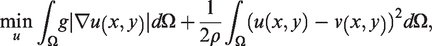
We review mainly the Roberts et al. ¹⁰ model, which is based on the framework of Chan and Vese ² and forms the basis of our proposed method. This model takes the following form

$$\begin{array}{l}\underset{\Gamma ,c_1,c_2}{\min }\{\text{length}(\Gamma )+\theta {\displaystyle {\int }_{{\Omega }_1}\mathcal{D}}\text{d}\Omega +{\lambda }_1{\displaystyle {\int }_{{\Omega }_1}(z(}x,y)-c_1{)}^2\text{d}\Omega \\ +{\lambda }_2{\displaystyle {\int }_{{\Omega }_2}(z(}x,y)-c_2{)}^2\text{d}\Omega \}\end{array}$$

(1)

where c₁ and c₂ are the average intensities inside ${\Omega }_1$ and ${\Omega }_2$ respectively, and $\mathcal{D}$ based on $\mathcal{M}$ and gradients of z is the geodesic distance constraint which will be discussed later.

In order to solve this model, as done in Chan and Vese, ² one uses the level set idea from Osher and Sethian ¹¹ to represent our l set idea fro $\varphi$ , i.e.

$$\varphi (x,y)=\{\begin{array}{l}>0,(x,y)\in {\Omega }_1,\hfill \\ =0,(x,y)\in \Gamma ,\hfill \\ <0,(x,y)\in {\Omega }_2.\hfill \end{array}$$

The model is reformulated to the form:

$$\begin{array}{l}\underset{\varphi ,c_1,c_2}{\min }{\displaystyle {\int }_{\Omega }g}|\nabla H_{\mathrm{ϵ}}(\varphi )|\text{d}\Omega +\theta {\displaystyle {\int }_{\Omega }\mathcal{D}}{H}_{\mathrm{ϵ}}(\varphi )\text{d}\Omega \\ +\lambda {\displaystyle {\int }_{\Omega }[}{(z-c_1)}^2{H}_{\mathrm{ϵ}}(\varphi )+{(z-c_2)}^2(1-H_{\mathrm{ϵ}}(\varphi ))]\text{d}\Omega \end{array}$$

(2)

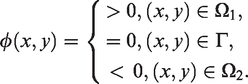
where we have set ${\lambda }_1={\lambda }_2=\lambda ,H_{\mathrm{ϵ}}(\varphi )=\frac{1}{2}\left(1+\frac{2}{\pi }\arctan \left(\frac{\varphi }{\mathrm{ϵ}}\right)\right)$ is the regularised Heaviside function, and $g=g(|\nabla z|)$ is the edge detector to the regulariser with $g(s)=\frac{1}{1+\beta s^2}$ . The inclusion of the Heaviside function results in our current functional being non-convex. This means a minimiser found could be a local minimum, and not a global minimum. The convex relaxation idea from Chan et al. ¹² provides a solution to this problem. It has been shown that the Euler-Lagrange equations for the minimisation of $\varphi$ have the same solutions to the following minimisation problem:

$$\begin{array}{l}\underset{u,c_1,c_2}{\min }{\displaystyle {\int }_{\Omega }g}|\nabla u|d\Omega +\lambda {\displaystyle {\int }_{\Omega }f}ud\Omega +\theta {\displaystyle {\int }_{\Omega }\mathcal{D}}u\text{d}\Omega \\ +\alpha {\displaystyle {\int }_{\Omega }\nu }(u)\text{d}\Omega ,\end{array}$$

(3)

where $f={(z-c_1)}^2-{(z-c_2)}^2$ and $\nu (u)=\max \{0,2|u-\frac{1}{2}|-1\}$ is a penalty term introduced in Chan et al. ¹² to ensure $u\in [0,1]$ . The global minimizer is ensured if c₁, c₂ are accurate which are often assured by the marker set and its associated initial contour.

We define the geodesic distance $\mathcal{D}$ taking the marker set $\mathcal{M}$ from the user, by solving the Eikonal equation

$$|\nabla \mathcal{D}(x,y)|=\mathrm{ϵ}+\beta |\nabla z(x,y){|}^2+\theta {\mathcal{D}}_E(x,y),$$

(4)

where ${\mathcal{D}}_E$ is the Euclidean distance away from $\mathcal{M}$ . We use a fast time sweeping method Zhao ¹³ to solve this equation, which requires setting $\mathcal{D}(x,y)=0$ for $(x,y)\in \mathcal{M}$ , and the calculation evolving from that region.

In order to perform the minimisation, we alternate between minimising c₁ and c₂ with u fixed, then with c₁ and c₂ fixed, we solve for u. Minimising with respect to c₁ and c₂ gives us

$$c_1=\frac{{\displaystyle {\int }_{\Omega }z}(x,y)u(x,y)\text{d}\Omega }{{\displaystyle {\int }_{\Omega }u}(x,y)\text{d}\Omega } ,c_2=\frac{{\displaystyle {\int }_{\Omega }z}(x,y)(1-u(x,y))\text{d}\Omega }{{\displaystyle {\int }_{\Omega }(1-u(}x,y))\text{d}\Omega }.$$

(5)

To minimise with respect to u with c₁ and c₂ fixed as above, we use the dual formulation by Chambolle, ¹⁴ which was first applied to a segmentation problem in Bresson et al., ¹⁵ by introducing a second variable, v, and alternating between the minimisation of u and v. In addition, it is shown in Bresson et al. ¹⁵ that the penalty term $\nu (u)$ is not necessary in this framework, provided that the initialisations $u^{(0)},v^{(0)}\in [0,1]$ . Our model then becomes

$$\begin{array}{l}\underset{u,v,c_1,c_2}{\min }{\int }_{\Omega }g|\nabla u(x,y\left)\right|\text{d}\Omega +\frac{1}{2\rho }{\int }_{\Omega }\left(u\right(x,y)-v(x,y){)}^2\text{d}\Omega \\ +{\int }_{\Omega }f(x,y,c_1,c_2)v(x,y)\text{d}\Omega ,\end{array}$$

(6)

where we re-define f by

$$f(x,y,c_1,c_2)=\lambda ({(z(x,y)-c_1)}^2-{(z(x,y)-c_2)}^2)+\theta \mathcal{D}(x,y),$$

and the new parameter $\rho >0$ is small. We first fix all variables except u and solve the u variational problem:

$$\underset{u}{\min }{\int }_{\Omega }g|\nabla u(x,y\left)\right|d\Omega +\frac{1}{2\rho }{\int }_{\Omega }\left(u\right(x,y)-v(x,y){)}^{2}d\Omega ,$$

which is given via the dual variable $p=(p_1,p_2)$

$$u=v-\rho \text{div}p$$

(7)

which is solved iteratively with $p^0=\mathbf{0}$ and

$$p^{n+1}=\frac{p^n+\delta t\nabla \left(\text{div}\left(p^n\right)-\frac{v}{\rho }\right)}{1+\frac{\delta t}{g\left(x\right)}|\nabla (\text{div}\left(p^n\right)-\frac{v}{\rho }|},$$

After updating and fixing u, we solve the v variational problem

$$\underset{v}{\min }\frac{1}{2\rho }{\int }_{\Omega }\left(u\right(x,y)-v(x,y){)}^2\text{d}\Omega +{\int }_{\Omega }f(x,y,c_1,c_2\left)v\right(x,y)\text{d}\Omega ,$$

(8)

by finding its analytical solution:

$$v(x,y)=\min \{\max \{u(x,y)-\rho f(x,y,c_1,c_2),0\},1\}.$$

(9)

A multiphase model

The traditional approach that can lead to an output approximating our desired result is to formulate the segmentation task as a multiphase problem. Then our solution will hopefully be an object that is comprised of two phases (though practically this may not be possible due to the non-convex nature of a multiphase model).

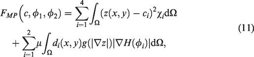
We briefly review the work of Vese and Chan, ¹⁶ which explains how to extend the traditional Chan and Vese ² framework to multiple level sets, providing a method of segmenting an image into multiple phases. Their four-phase model using two level set functions, ${\varphi }_1$ and ${\varphi }_2$ , to segment an image is the following:

$$\begin{array}{l}{F}_{MP}(c,{\varphi }_1,{\varphi }_2)=\sum _{i=1}^4{\int }_{\Omega }\left(z\right(x,y)-c_i{)}^2{\chi }_{i}d\Omega \\ +\sum _{i=1}^2\mu {\int }_{\Omega }|\nabla H({\varphi }_i\left)\right|d\Omega ,\end{array}$$

(10)

where $c=(c_{11},c_{10},c_{01},c_{00})$ is a constant vector and

$${\chi }_1=H\left({\varphi }_1\right)H\left({\varphi }_2\right),{\chi }_2=H\left({\varphi }_1\right)(1-H({\varphi }_2\left)\right),{\chi }_3=(1-H({\varphi }_1\left)\right)H\left({\varphi }_2\right),$$

and ${\chi }_4=(1-H({\varphi }_1))(1-H({\varphi }_2)).$

We note however that this model achieves global segmentation, and therefore using this model wons. Their four-phase model using two lev Figure 1(o). To restrict the two level sets from segmenting objects outside the objects of interest, we merge ideas from Gout et al. ⁶ and Badshah and Chen, ⁷ by adding two distance constraints d₁, d₂, and edge detector g into the regularisors of the above model:

$$\begin{array}{l}{F}_{MP}(c,{\varphi }_1,{\varphi }_2)=\sum _{i=1}^4{\int }_{\Omega }\left(z\right(x,y)-c_i{)}^2{\chi }_i\text{d}\Omega \\ +\sum _{i=1}^2\mu {\int }_{\Omega }{d}_i(x,y)g\left(\right|\nabla z\left|\right)|\nabla H({\varphi }_i\left)\right|\text{d}\Omega ,\end{array}$$

(11)

where we require two marker sets ${\mathcal{M}}_i$ , i = 1, 2, for the computation of the two new distance constraints d_i, which is given by:

$$d_i(x,y)=\left(1-e^{\frac{{(x_j-x)}^2}{2{\sigma }^2}}{e}^{\frac{{(y_j-y)}^2}{2{\sigma }^2}}\right), \text{ for } (x_i,y_i)\in {\mathcal{M}}_i.$$

In Figure 2, we perform the above multiphase model to the image in Figure 1, with the aim of achieving the result in Figure 1(o). We first show the input required in Figure 2(a), and the result in (b). First, we note that the required input for the multiphase model is detailed (whereas the proposed method which we detail in the next section requires just a single click), as the multiphase method is non-convex, and therefore we need the initialisation to be close to the final solution. A single click by the user is unlikely to be enough information for a non-convex model such as this to reliably work. Despite the increased input, we can see that while the multiphase has successfully segmented the first region correctly, the second level set has failed to make its way around the lower left side of the second region.

Figure 2.

Input and output of the multiphase model. (a) Input. Red: ${\mathcal{M}}_1$ , Blue: ${\mathcal{M}}_2$ . (b) Multiphase out.

In the following section we detail our proposed method, which makes use of the convex segmentation model (3) and an in-painting method to segment an object or feature of two distinct intensities.

The new model

We now present our model for the segmentation problem where an interested object or feature in the given image z has two distinct intensities. We first give a general formulation and then consider a simplified version and its special cases.

A general formulation

Consider the aorta and stent problem in top row of Figure 3 to define the notation. Given image z (as in the left plot), our task is to segment the complete organ defined by ${\Omega }_1$ (for the aorta in the right plot). Here a marker set $\mathcal{M}$ is placed in the domain ${\Omega }^{*}$ and laced in the domain gdomain ${\Omega }_1$ . Also we have ${\Omega }^{*}\subset {\Omega }_1\subset \Omega$ while ${\Omega }_1{\displaystyle \cup \Gamma }{\displaystyle \cup {\Omega }_2}=\Omega$ .

Figure 3.

Illustration of the task of segmentation of the outer organ ${\Omega }_1$ (aorta) distracted by the inner feature ${\Omega }^{*}$ of a stent, with $\Gamma =\partial {\Omega }_1$ and also inpainted images by TV and Elastica models. (a) Given image. (b) Segmentation of domain Ω₁. (c) Inpainted image by TV. (d) Inpainted image by Elastica.

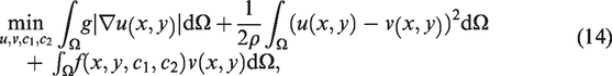
The biggest challenge is that the intensities in ${\Omega }^{*}$ are dominant and would prevent us from locating Γ of ${\Omega }_1$ , our idea is to inpaint the intensities in ${\Omega }^{*}$ using neighboring information to obtain an in-painted image $z^{*}$ , and segment the main feature in ${\Omega }_1$ at the same time. Hence our segmentation takes the form

$$\begin{array}{l}\underset{z^{*},u,v,c_1,c_2}{\min }\frac{{\alpha }_1}{2}{\int }_{\Omega \backslash {\Omega }^{*}}{(z^{*}-z)}^{2}d\Omega +{\alpha }_2{\int }_{\Omega }|\nabla z^{*}(x,y\left)\right|u(x,y)\text{d}\Omega \\ +{\int }_{\Omega }g|\nabla u(x,y\left)\right|d\Omega +\frac{1}{2\rho }{\int }_{\Omega }\left(u\right(x,y)-v(x,y){)}^2\text{d}\Omega \\ +{\int }_{\Omega }f(x,y,c_1,c_2)v(x,y)\text{d}\Omega ,\end{array}$$

(12)

where $f(x,y,c_1,c_2)=\lambda ({(z^{*}(x,y)-c_1)}^2-{(z^{*}(x,y)-c_2)}^2)+\theta \mathcal{D}(x,y)$ similar to but different from (6). Here regularisation in the second term in the domain ${\Omega }_1$ may be replaced by the whole domain Ω. Since ${\Omega }^{*}\subset {\Omega }_1\subset \Omega$ for our type of problems, in fact, it is not difficult to see that $z^{*}=z$ in ${\Omega }_2=\Omega \backslash {\Omega }_1$ .

A remark is due for the second term in (12): the use of total variation for inpainting is generally a poor choice Chan and Shen ¹⁷ ; Schönlieb ¹⁸ while the elastica based model Brito and Chen ¹⁹ is better. Here the assumption ${\Omega }^{*}\subset {\Omega }_1\subset \Omega$ implies that there are no extra edges in ${\Omega }^{*}$ to reconnect and hence our inpainting problem is much easier than the general case where ${\Omega }^{*}$ cuts cross major features. In fact, the bottom row of Figure 3 show the results from applying the TV and the elastica models; clearly the results are good (though it takes relatively a long time to obtain such results) but not excellent due to the inpainted values of $z^{*}$ differing from neighbours.

The domain ${\Omega }^{*}$ itself is usually not given but since the associated intensities are dominant, we can assume that it can be obtained.

Below we discuss how to simply (12) so that other models to inpaint ${\Omega }^{*}$ can be developed.

A simplified model

Although image z has many features, our selective segmentation aims to segment one feature i.e. to find the domain ${\Omega }_1$ by working with the new image $z^{*}$ after inpainting ${\Omega }^{*}$ . As mentioned, the key to simplify the model (12) lies in two related facts: i) ${\Omega }^{*}\subset {\Omega }_1\subset \Omega$ ; ii) there are no extra edges in ${\Omega }^{*}$ to reconnect. This leads to our 2-stage model.

Stage 1 tage 1onnect. of $z^{*}$ . From (12), solution $z^{*}$ is approximated by

$$\underset{z^{*}}{\min }{\int }_{\Omega }|\nabla z^{*}(x,y\left)\right|u(x,y)\text{d}\Omega ={\int }_{{\Omega }_1}|\nabla z^{*}(x,y\left)\right|\text{d}\Omega ,$$

(13)

since u = 1 in ${\Omega }_1$ . In the next subsection, we propose various ways of approximating $z^{*}$ .

Stage 2. Once $z^{*}$ is computed, (12) is reduced to a standard model for selective segmentation of the inpainted image $z^{*}$ , i.e.

$$\begin{array}{l}\underset{u,v,c_1,c_2}{\min }{\int }_{\Omega }g|\nabla u(x,y\left)\right|\text{d}\Omega +\frac{1}{2\rho }{\int }_{\Omega }\left(u\right(x,y)-v(x,y){)}^2\text{d}\Omega \\ +{\int }_{\Omega }f(x,y,c_1,c_2)v(x,y)\text{d}\Omega ,\end{array}$$

(14)

Methods for computing $z^{*}$

Let us assume we have obtained our first segmentation result, $u^{*}$ to represent ${\Omega }^{*}$ , using the method discussed in section 2. In this modified Chan-Vese framework, the indicator function $u^{*}$ is associated with c₁ (the average value of the intensity inside ${\Omega }^{*}$ and c₂ (the average value of the intensity outside ${\Omega }^{*}$ ).

Then for Stage 1, we discuss several ways of computing $z^{*}$ in ${\Omega }^{*}$ since $z^{*}=z$ in $\Omega \backslash {\Omega }^{*}$ .

Method M1. It may be intuitive to threshold our region down to the value of c₂. However, typically c₂ is the average of intensities in $\Omega \backslash {\Omega }^{*}$ , not exactly representative of the surrounding intensities in ${\Omega }_1$ . We denote the method of thresholding to c₂ as M1. See Figure 4.

Figure 4.

M1 –1g.ticay Elastica Elc₂. The original image is displayed on the top row, and the in-painted image is shown on the bottom.

Method M2. As demonstrated in Figure 4, c₂ is perhaps not the most ideal to use for complicated images. To go beyond a constant intensity, we propose to use the variance of a region (by Jeon et al. ²⁰ ):

$$\mathit{Var}\left(I_i\right)=\frac{1}{N_i}\sum _{j=1}^{N_i}\left(I_i\right(x_j,y_j)-m_i{)}^2,$$

assuming m_i is the mean intensity of one of region I_i (with N_i pixels) in partition of a given image I. For our case, we obtain 2 regions I₁, I₂ after segmenting ${\Omega }^{*}$ , and compute the $\mathit{Var}(I_2)$ . Then we inpaint ${\Omega }^{*}$ by a normal distribution with mean c₂ and variance $\mathit{Var}(I_2)$ . Let us denote this method as M2, however this is not much of an improvement from M1 as shown in Figure 5.

Figure 5.

M2 —2Thresholding using $c\sim N(c_2,\mathit{var}(I_2))$ . Original image desiplayed on the top row, and the in-painted image is shown on the bottom.

Method M3. Since c₂ is not informative due to $\Omega \backslash {\Omega }^{*}$ being a large and nonhomogeneous region, we consider a local region surrounding ${\Omega }^{*}$ instead. We can obtain a more accurate threshold value by making use of the segmentation result $u^{*}$ and the associated region ${\Omega }^{*}$ . We extend ${\Omega }^{*}$ out by $\ell$ pixels as shown in Figure 6(b) (we typically fix $\ell =5$ ) and obtain a fix region or ${\Omega }^{*}$ , denoted as Ω _ring , given by ${\Omega }_{\mathit{ring}}={\Omega }^{\ell }\backslash {\Omega }^{*}$ , as shown in Figure 6(c).

Figure 6.

The ring region Ω _ring by extending ${\Omega }^{*}$ . (a) ${\Omega }^{*}$ . (b) ${\Omega }^{\ell }$ . (c) Ω _ring .

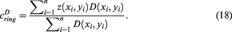
We simply calculate the average intensity c_ring of pixels contained in Ω _ring , and inpaint our region ${\Omega }^{*}$ down to this intensity. This gives us an image in which our first region is now representative of our second target region, allowing us to perform another segmentation, as shown in Figure 7. We will denote this method as M3.

Figure 7.

M1-3 1-3Both segmentof inpainting ${\Omega }^{*}$ by a constant intensity (visually not pleasing in column 1 but leading to Stage 2he bottomottom.development of computer assisted automated disease diagnostic . (a) Thresholded image. (b) Segmentation u₂. (c) Both segmentations. (d) Thresholded image. (e) Segmentation u₂. (f) Both segmentations.

Method M4. The above three methods can lead to successful Stage 2 segmentation on the new inpainted image in our tests. However, the inpainted region by thresholding to a constant intensity is visually visible in the inpainted image. To improve the visual quality, we consider the idea of M2 by the Normal distribution. We threshold each pixel in ${\Omega }^{*}$ individually to a number drawn from the normal distribution, with mean c_ring and variance in Ω _ring calculated as defined earlier. Denote this by M4.

Method M5. M4 may give good aesthetic results in some cases, for example in Figure 9 where we see it replicates the texture of the blood vessel very well, however for a homogeneous ${\Omega }_1$ , the normal distribution is unlikely to perform well and the image would look out of place. In order to replicate the texture of the surrounding pixels, a simple method would be to just copy and paste values of pixels in the ring to ${\Omega }^{*}$ inwards, repeating the sequence until all of ${\Omega }^{*}$ has been filled in. Here, we can either fill the pixels in row by row (Figure 8(a)), by spiralling inwards towards the center of ${\Omega }^{*}$ (Figure 8(b)), or completely randomly (Figure 8(c)). We recommend to fill in randomly, so that we don we dony, so that we donxels in row b occurring in the texture of the in-painted region.

Figure 8.

M5 5g.Randomlingntationsty (visualinpainting. (a) Row by row. (b) Spiralling. (c) Random.

In principle, the choice between M3-5 should not have too much of an effect on the second segmentation result as the average value of the region ${\Omega }^{*}$ after applying a particular method should be very similar to the average value of applying another. Figure 9 shows a comparison between using each method. A second segmentation is easily achievable using either. Visually we recommend a variant of M5.

Figure 9.

Comparison between M3 (constant), M4 (normal distribution) and M5 (inward extension). (a) M3. (b) M4. (c) M5. (d) M3. (e) M4. (f) M5.

Variational comparisons

In this section we make a comparison to two traditional variational in-painting methods detailed in Schönlieb, ¹⁸ firstly the Mumford-Shah method given by minimising the following energy:

$$\begin{array}{l}{F}_{MS}(z^{*},\chi )=\frac{1}{s}\left|\right|z^{*}-z|{|}_{L^s(\Omega \backslash {\Omega }^{*})}^s+\frac{\alpha }{2}{\int }_{\Omega }\chi |\nabla z^{*}{|}^2\text{d}\Omega \\ +\beta {\int }_{\Omega }\left(\mathrm{ϵ}\right|\nabla \chi {|}^2+\frac{{(1-\chi )}^2}{4\mathrm{ϵ}})\text{d}\Omega ,\end{array}$$

(15)

where χ is an approximation of the edges in the image introduced in Ambrosio and Tortorelli. ³

In addition, wee:///\\\\chenas03.cadmus.com\\smartedit\\Normalization\

$$\underset{z^{*}\in H^1\left(\Omega \right)}{\min }{\int }_{{\Omega }^{*}}|\nabla z^{*}{|}^{2}d\Omega \text{ , such that }{z}^{*}=z\in \Omega \backslash {\Omega }^{*}.$$

(16)

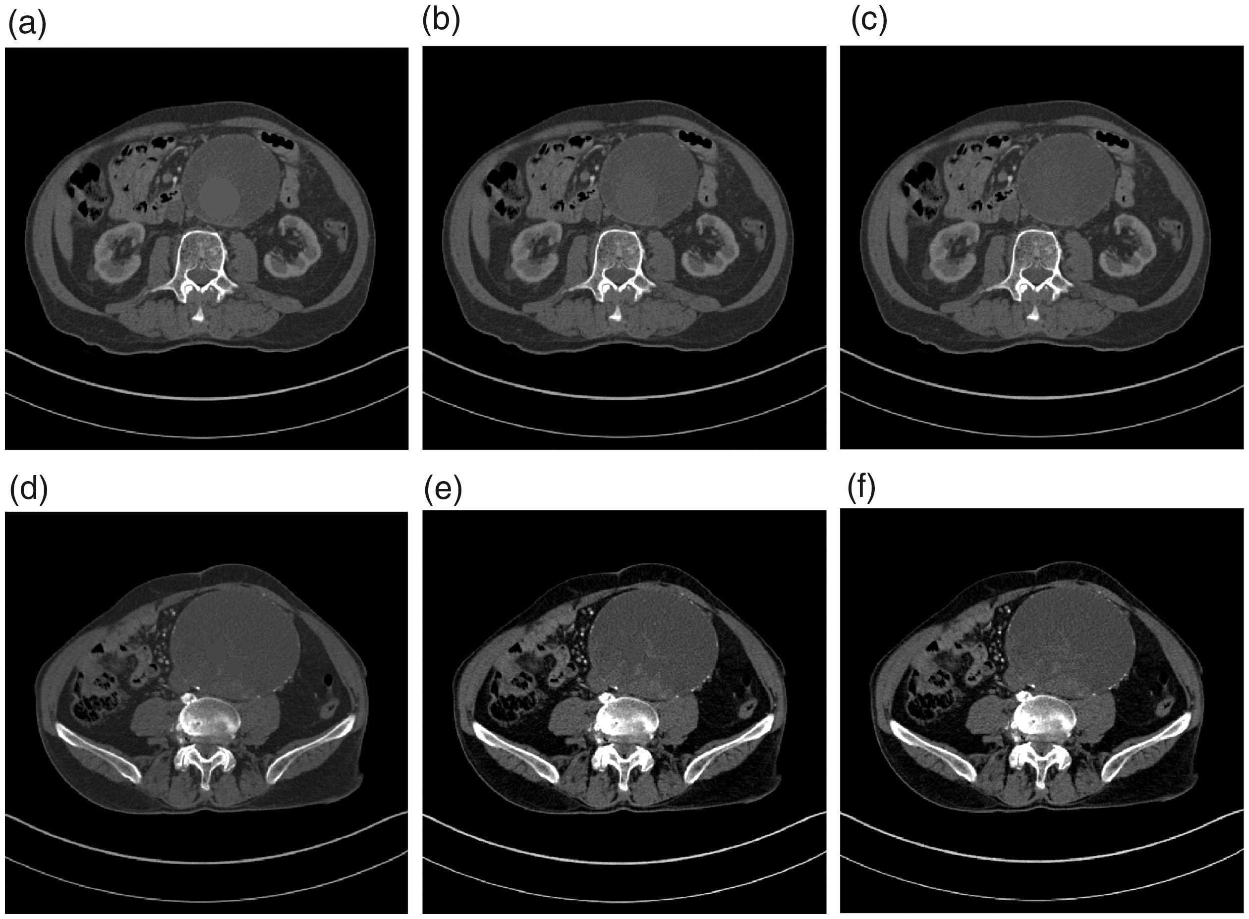
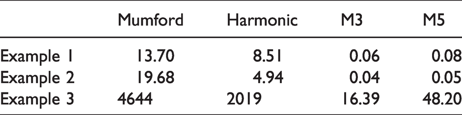
We consider three examples in total, showing the output for the first two examples in Figure 10, and the corresponding results using our methods are found in Figures 9 and 15 respectively. Example 3 is a large pathological colour image of dimension 9863 × 11,454 which we have tested for the sake of measuring the computation speed. Computation speed is given in Table 1. We see that, although the variational methods give similar results to our M3 and would therefore be suitable to use as an input for our second segmentation stage, the computation time is much larger. The in-painting step in our method is an intermediate step which allows us to obtain a second segmentation result, therefore speed is the only thing we should be concerned with.

Figure 10.

$z^{*}$ using variational inpainting models. (a) Ex1: Mumford-Shah output. (b) Ex1: Harmonic output. (c) Ex2: Mumford-Shah output. (d) Ex2: Harmonic output.

Table 1.

Speed (seconds) of each in-painting method.

	Mumford	Harmonic	M3	M5
Example 1	13.70	8.51	0.06	0.08
Example 2	19.68	4.94	0.04	0.05
Example 3	4644	2019	16.39	48.20

Distance weighted in-painting

The above recommended method M5 (and also others for this matter) would fail to yield an acceptable inpainted image if ${\Omega }^{*}$ and ${\Omega }_1$ share part of a boundary, because the threshold value out of the region surrounding ${\Omega }^{*}$ will be influenced by the intensity of both the second object desired and a neighbouring objects. We now address the mathematical challenge below by modifying the $\ell$ band in M3-5. This scenario can occur in practical images e.g. when diseases are present near the boundary of an organ.

It is possible to accommodate this particular case if a specific application occurs in the same position all the time, for example if object one is always on the left boundary of object two, we could simply just consider the average intensity of pixels in the right hand ring. However, for a general application we need an alternative solution.

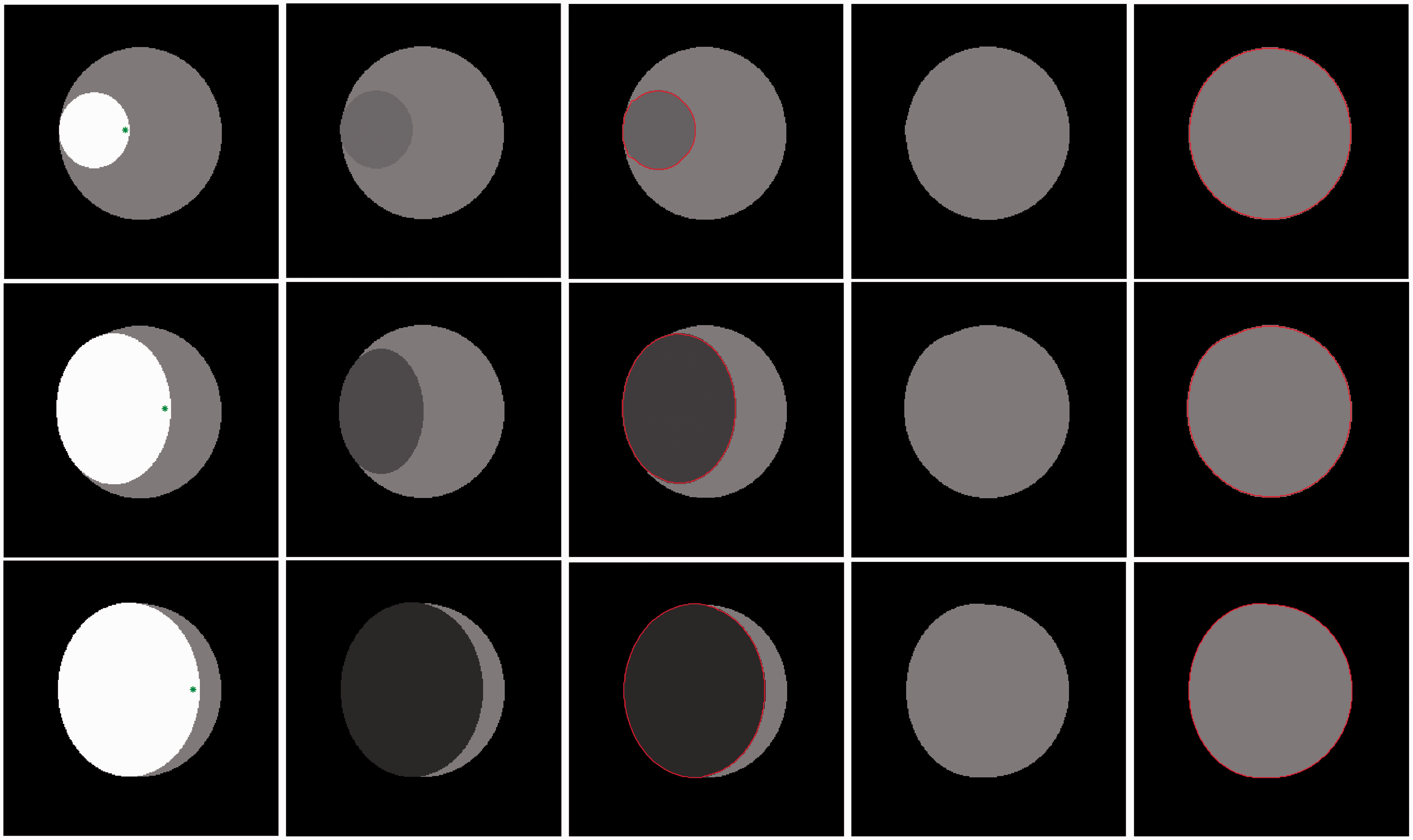
The second column of Figure 11 demonstrates the problem at the boundary using synthetic images. The more domain ${\Omega }^{*}$ touches the boundary/unwanted region, the smaller(darker) the threshold value within $\ell$ band becomes and the less suitable the region becomes for a second segmentation result.

Figure 11.

Column 1: Original image with user input. Column 2: Inpainted by M3. Column 3: Associated segmentation result from column two result. Column 4: Inpainted by our distance weighted method we present in section 4. Column 5: Associated segmentation result from column three result.

An easy solution would be to retrieve another marker from the user, indicating the second region, however this defeats the whole purpose of our method of segmenting two objects with one click. An alternative solution would be to ask the user to input their marker inside the first object close to the boundary between the two objects desired. Using this information, we can change our methods slightly.

M3 revisited: Instead of taking the average intensity of values near ${\Omega }^{*}$ , we could apply a weight to the intensities according to a weight function. The weight is designed to have a higher value for pixels close to the marker (i.e. the intensities of object two in ${\Omega }_1\backslash {\Omega }^{*}$ ). We use the Euclidean distance to weight the pixels. We consider $D(x,y)\in [0,1]$ to be the normalised Euclidean distance from the marker(s) $(x_{\mathcal{M}},y_{\mathcal{M}})$ to pixels contained in Ω _ring

$$D(x,y)=\{\begin{array}{l}\frac{\sqrt{{(x-x_{\mathcal{M}})}^2+{(y-y_{\mathcal{M}})}^2}}{\left|\right|\sqrt{{(x-x_{\mathcal{M}})}^2+{(y-y_{\mathcal{M}})}^2}|{|}_{L^{\infty }}},(x,y)\in {\Omega }_{\mathit{ring}},\hfill \\ 0,\text{otherwise},\hfill \end{array}$$

(17)

we can define c_ring to threshold the region by

$$c_{\mathit{ring}}^D=\frac{{\displaystyle {\sum }_{i=1}^{n}z}(x_i,y_i)D(x_i,y_i)}{{\displaystyle {\sum }_{i=1}^{n}D}(x_i,y_i)}.$$

(18)

This makes the thresholding value to be more representative of the second object, and so the Chan-Vese fitting term is more likely to work.

For difficult images, it might be more accurate to change our weighting function to only consider the closest, say 20%, pixels in Ω _ring , rather the entire region. Depending on the application this amount could change. We recommend only considering the nearest 20% of all pixels regardless, as this will provide a more realistic value; there is no reason to consider the furthest pixels away contained Ω _ring .

We see in Figure 11 in column 4, that with this new method, the inpainted image is much more representative of the second object, and isnag influenced by the black background. In Figure 12 we see the model work on the boundary even with an awkward shape.

Figure 12.

Using 20% as weight. (a) ${\Omega }^{*}$ and marker placement $\mathcal{M}$ . (b) Second segmentation. (c) Combined segmentation.

M5 revisited: The discussion so far shows an extension of M3 to manage in the case where ${\Omega }^{*}$ is near the boundary of ${\Omega }_1$ . In the synthetic images, performance is great, however using a single constant value to threshold ${\Omega }^{*}$ leads to a visible awkward looking region as is discussed in the previous section. Instead of extending M3, we can extend M5 in a similar way to attempt to maintain some of the texture of ${\Omega }_1$ . To do this, instead of copying and pasting the values of all the pixels in Ω _ring , we can set a cut off point, say, only copy 20% of the closest pixels to the marker point contained in Ω _ring .

Algorithmic summaries

Finally we summarise the main algorithms. All three algorithms must be used to find the two segmentations that we desire.

Algorithm 1 Segmentation algorithm

Input image z and parameters $\lambda ,\theta$ and ρ.

Calculate g and ${\mathcal{D}}_G$ .

Initialise $u^{(0)}$ such that se s orithmAll throf $\mathcal{M}$ .

for $k=1:\mathit{maxit}$ do

Update $c_1^{(k)}(u^{(k-1)}),c_2^{(k)}(u^{(k-1)})$ as in (5).

Update u^k and v^k as in (7) and (9) respectively

end for

$u\leftarrow u^{(k)}$ and set ${\Omega }_1=\{(x,y)|u(x,y)\ge 1/2\}$

(2) To inpaint domain ${\Omega }^{*}$ , based on $\mathbf{M}\mathbf{5}$ (other methods similar, see previous sections for details), we do the following:

Algorithm 2 Inpainting step M5

Input image z and domain to be inpainted ${\Omega }^{*}$ .

Initialise inpainted image $z^{*}:=z$ .

Obtain ${\Omega }^{\ell }$ by extending ${\Omega }^{*}$ out by $\ell$ pixels. Use ${\Omega }^{\ell }$ to find ${\Omega }_{\mathit{ring}}={\Omega }^{\ell }\backslash {\Omega }^{*}$ .

Collect intensity values of the nearest 20% of pixels in Ω _ring to $\mathcal{M}$ in a vector v.

for $(x,y)\in {\Omega }^{*}$ do

Update $z^{*}(x,y)=v(i)$ .

$i=i+1$ . If $i>\mathit{size}(v)$ , set i = 1.

End for

Output inpainted image $z^{*}$ .

(3) Finally we make use the same input $\mathcal{M}$ and segment the inpainted image $z^{*}$ .

Algorithm 3 Proposed two stage segmentation algorithm to segment and object or feature of two distinct intensities.

Input initial image z₁ and parameters ${\lambda }_1,{\theta }_1$ and ρ₁ to perform segmentation by algorithm 1, obtaining initial segmentation region ${\Omega }^{*}$ as output.

Input z₁ and ${\Omega }^{*}$ into algorithm 2 to inpaint the image, yielding z₂.

Input z₂ and parameters ${\lambda }_2,{\theta }_2,{\rho }_2$ to perform algorithm 1 again, this time using ${\Omega }^{*}$ as our initialisation.

Output ${\Omega }^{*}$ and ${\Omega }_1$ , two segmented regions.

(4) If we have a case in which our desired ${\Omega }_1$ has more than two distinct intensities contained inside it and running algorithm 3 outputs segmented regions capturing only two of the distinct regions, then we can instead in-paint the image and segment iteratively until the desired result is achieved. See Figure 15 for an example. In some cases, we could in principle use our method to hierarchically segment an entire image by iteratively segmenting and in-painting.

Numerical experiments

In this section we will demonstrate some results illustrating the principle of our method. With the geodesic distance, only a single point is required from the user inside the initial region of interest (however if the initial region ${\Omega }^{*}$ is disconnected, we need one click in each disconnected region). From that we obtain segmentation of the region, a thresholded image, and another segmentation performed on the new image. In all tests we set parameters from the segmentation model ρ = 1 and $dt=\frac{1}{8}$ , and for calculating the geodesic distance we fix $\mathrm{ϵ}={10}^{-3},\beta =1000$ and $\theta =0.1$ . This leaves us with only the λ and θ values in the segmentation model to vary.

Example 1: Disconnected stent

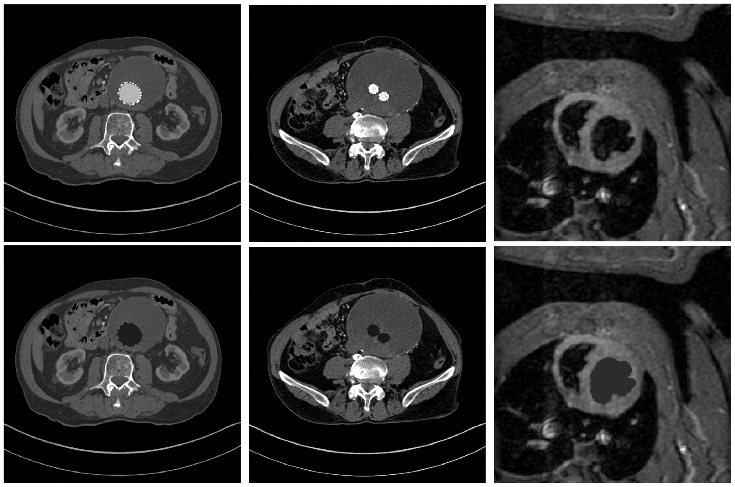
Figures 13 and 14 show a stent in an abdominal aortic aneurysm, with both images being 512 × 512. We would like to know the position of the stent relevant to the surrounding blood vessel, so this method lends itself well. Two clicks were required for the second image in Figure 13 as the stent is disconnected. From this, we obtain a realistic in-painted image with which we can perform a second segmentation and obtain very accurate results quickly.

Figure 13.

Stent in an abdominal aortic aneurysm. (a) Original image, z₁. (b) User input, $\mathcal{M}$ . (c) ${\Omega }^{*}$ . (d) Inpainted image. (e) Ω₁. (f) ${\Omega }^{*}$ and ${\Omega }_1$ .

Figure 14.

In this example we demonstrate the use of in-painting twice, requiring three segmentations due to the bright noise between the stent and the boundary of the blood vessel. (a) First segmentation, ${\Omega }_1^{*}$ . (b) First in-painted image z₂. (c) Second segmentation, ${\Omega }_2^{*}$ . (d) Second in-painted image z₃. (e) Third segmentation, ${\Omega }_1$ . (f) ${\Omega }_1^{*}$ and ${\Omega }_1$ .

Example 2: Stent with noise - multiple in-paintings

Figure 14 demonstrates using the method twice to obtain segmentation of the blood vessel. In this case there is noise present produced by the metal coated stents causing the interior of the aorta to be brighter than the rest of it. This example is different to the previous one as there are three distinct intensities contained in our desired ${\Omega }_1$ (the boundary of the blood vessel), due to noise. Therefore, we are required to segment and in-paint twice, before segmenting finally to obtain ${\Omega }_1$ . We use ${\lambda }_1={\lambda }_2={\lambda }_3=5$ and ${\theta }_1={\theta }_2={\theta }_3=20$ . This example requires one more in-painting step than what has been discussed

Example 3: Stent on boundary

We show another stent in an abdominal aortic aneurysm in Figure 15, in which ${\Omega }^{*}$ is lying on the boundary of ${\Omega }_1$ . In this case, it is important that the methods discussed in section 4 are implemented, as otherwise our inpainted image would be not be suitable for a second segmentation. The placement of the marker is placed as close to ${\Omega }_1$ as possible while still contained in ${\Omega }^{*}$ , as shown in Figure 15(b), and when we in-paint we only consider the closest 20% of pixels contained in Ω _ring .

Figure 15.

This figures shows a stent in an abdominal aortic aneurysm. In this case, ${\Omega }^{*}$ is touching the boundary of ${\Omega }_1$ . It is necessary in this case for the methods discussed in section 4 to be implemented, in order to obtain an appropriated in-painted image for an accurate ${\Omega }_1$ to be obtained. (a) Original image, z₁. (b) User input, $\mathcal{M}$ . (c) First segmentation, ${\Omega }^{*}$ . (d) In-painted image, z₂. (e) Second segmentation, Ω₁. (f) ${\Omega }^{*}$ and ${\Omega }_1$ .

Example 4: Ventricular walls

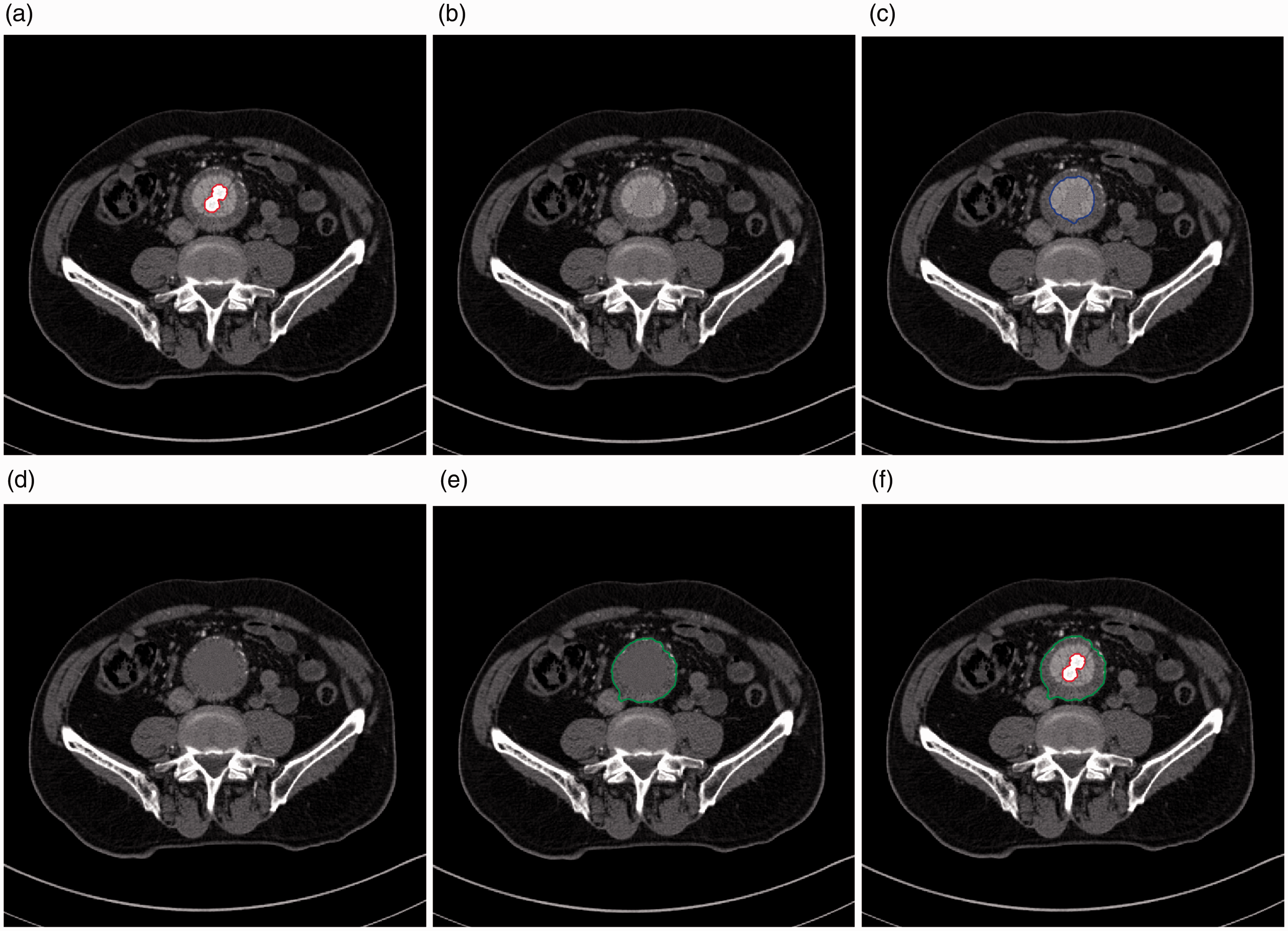
Figure 16 show an MRI of the heart of a rat. The method required clicking once in the two chambers (the dark regions inside the red contours of Figure 16(a)), which allowed us to obtain the inside region. We then inpainted choosing simply use $\mathbf{M}\mathbf{3}$ for this example, which allowed us to find ${\Omega }_1$ , the outline of the ventricular walls. The image size is small at 192 osing simply use s (the dark regions inside the red cont seconds. We use parameters ${\lambda }_1=1,{\theta }_1=20,{\lambda }_2=0.5,{\theta }_2=1.$

Figure 16.

Segmentation of MRI of a rat’s heart. (a) First segmentation, ${\Omega }^{*}$ . (b) Inpainted image, z₂. (c) Second segmentation, Ω₁. (d) ${\Omega }^{*}$ and ${\Omega }_1$ .

Example 6: Extension to colour

We show a brief example of our model being applied to a colour pathological image of multiple myeloma, given by Gupta and Gupta ²¹ ; Gupta et al.^22,23 So far we have only presented our method working for greyscale images, however it is easy to extend the framework to RGB. First the segmentation model (3) differs as we now have a vector valued image.

Let z_i be the ith channel of image z, i = 1, 2, 3 (in this example we have an RGB image), and let $c_1=(c_1^1,c_1^2,c_1^3)$ and $c_2=(c_2^1,c_2^2,c_2^3)$ be vectors corresponding to the average intensity inside and outside of Γ in each channel. We can therefore compose our fitting and distance term as $f_i={(z_i-c_1^i)}^2-{(z_i-c_2^i)}^2$ and ${\mathcal{D}}_i$ , where the calculation in (4) is calculated on z_i. Our equivalent colour segmentation model is now:

$$\begin{array}{l}\underset{u,c_1,c_2}{\min }{\displaystyle {\int }_{\Omega }g}|\nabla u|d\Omega +\lambda {\displaystyle \sum _{i=1}^3(}{\displaystyle {\int }_{\Omega }{f}_i}ud\Omega +\theta {\displaystyle {\int }_{\Omega }{\mathcal{D}}_i}ud\Omega )\\ +\alpha {\displaystyle {\int }_{\Omega }\nu }(u)d\Omega \end{array}$$

(19)

The in-painting step only differs in that the values of the pixels we fill in with are vector valued, like our image, so we just fill in the corresponding each channel separately with values from the vector valued pixels from Ω _ring .

Figure 17 shows a cell on the boundary, in which it is necessary to have employed our distance technique, involving placing the marker point $\mathcal{M}$ as close as possible to the second object (the light blue ellipse), but still inside the first (the purple circle).

Figure 17.

Colour example. (a) Original image, z₁. (b) User input, $\mathcal{M}$ . (c) First segmentation, ${\Omega }^{*}$ . (d) In-painted image, z₂. (e) Second segmentation, Ω₁. (f) ${\Omega }^{*}$ and ${\Omega }_1$ .

Example 7: Extension to 3D

Our inpainting method is easy to extend to 3D data, differing only is our image domain $\Omega \subset {ℝ}^3$ . Our segmentation model (3) extends easily to a third dimension, however of course our segmentation results ${\Omega }^{*}$ and ${\Omega }_1$ are now surfaces. The geodesic distance is solved using (4) with an extra dimension, and the method of solving the PDE is slightly different to the two-dimensional case, however the details are, again, contained in Zhao. ¹³

In principle the in-painting method is the same as in two-dimensions. To achieve M5, we perform segmentation to achieve a surface ${\Omega }^{*}$ , extend the surface outwards in the normal direction to obtain ${\Omega }^{\ell }$ , and then obtain ${\Omega }_{\mathit{ring}}={\Omega }^{\ell }\backslash {\Omega }^{*}.$ Note that despite Ω _ring not really being a ring in three dimensions, we keep the notation consistent to avoid confusion. We then take the intensity of voxels contained in Ω _ring , and use these intensities to fill in our region ${\Omega }^{*}$ as before.

Figure 18 shows a selection of slices of a 3D data set of an abdominal aortic aneurysm with a stent present. This particular set was done on image data of size $512\times 512\times 60$ , with a single click required to obtain an intial segmentation of the stent, ${\Omega }^{*}$ . From that we can obtain our in-painted 3D image and segment again, achieving a result for the blood vessel. In this particular example, as shown by the images, the stent begins as a single connected object at the top of the image data (top row), and in the middle bifurcates and disconnects into two seperate regions. The placement of the marker can be placed arbitrarily in any slice, regardless if on that particular slice the stent is disconnected, as in 3D the object is connected. To speed up the calculation of the geodesic distance, we place a marker on the top slice and two markers on the bottom, however in principle this result is achievable with a single click.

Figure 18.

Nine slices from a 3D dataset.

Conclusion

In this paper, we have presented a method of obtaining a second segmentation result from a segmented region without any further user interaction. We do this using a two stage approach, by segmenting an object, intelligently inpainting our image with a similar intensity to the object surrounding the segmented object, and performing the segmentation model a second time to obtain the surrounding object. We have compared and contrasted it to alternative approaches such as multiphase segmentation methods, and classic variational in-painting methods, and saw improved performance and ease of use contrasted to the former, and drastic speed increase contrasted to the latter.

A number of quick in-painting method have been discussed, all based on the same principle of using information from surrounding region Ω _ring . We have discussed the potential challenges of using these methods when the initial object ${\Omega }^{*}$ is on the boundary of ${\Omega }_1$ , and have suggested a potential solution with appropriate placement of the marker point $\mathcal{M}$ . We have then tested on many piecewise constant images, showing the effectiveness of our proposed method, as well as detailing an extension to both colour images, and 3D data.