A subspace type incremental two-dimensional principal component analysis algorithm

Abstract

Principal component analysis (PCA) has been a powerful tool for high-dimensional data analysis. It is usually redesigned to the incremental PCA algorithm for processing streaming data. In this paper, we propose a subspace type incremental two-dimensional PCA algorithm (SI2DPCA) derived from an incremental updating of the eigenspace to compute several principal eigenvectors at the same time for the online feature extraction. The algorithm overcomes the problem that the approximate eigenvectors extracted from the traditional incremental two-dimensional PCA algorithm (I2DPCA) are not mutually orthogonal, and it presents more efficiently. In numerical experiments, we compare the proposed SI2DPCA with the traditional I2DPCA in terms of the accuracy of computed approximations, orthogonality errors, and execution time based on widely used datasets, such as FERET, Yale, ORL, and so on, to confirm the superiority of SI2DPCA.

Introduction

The feature extraction is one of the most popular fields in computer vision and pattern recognition over the past three decades.^1–3 As an increase in the image information, a large amount of high-dimensional observation data are followed. ⁴ If we directly deal with high-dimensional data, we will face the problem of “dimensionality disaster”. ⁵ Thus, lots of dimensionality reduction algorithms have been proposed, such as Principal Component Analysis (PCA),^6,7 Linear Discriminant Analysis (LDA), ⁷ Neural Networks (NN), ⁸ Canonical Correlation Analysis (CCA) ⁹ and so on. PCA is one of the most well-known feature extraction and dimension reduction methods for high-dimensional data analysis.^10,11 In the online learning system, it is usually developed into the incremental PCA algorithm to alleviate the increasing numerical difficulties in computational costs, memory demands, and numerical stability.

Denote the data set in the form of the data matrix $X\in {ℝ}^{d\times n}$ , where d is the dimension of the data set and n is the number of data points in the data set. Without loss of generality, we assume X is centered, i.e., $X{1}_d=0$ , where $1_d\in {ℝ}^d$ is the vector of all ones, otherwise, we can preprocess X as $X\leftarrow X-\frac{1}{d}X{1}_d$ . To reduce the dimension of X from d to k where $k\ll d$ , PCA aims to find the first k principal eigenvectors corresponding to the first k largest eigenvalues of the covariance matrix $\Sigma =X{X}^{\text{T}}$ , ¹² and then projects the high-dimensional data onto the k-dimensional subspace spanned by these principal eigenvectors to achieve the purpose of dimensionality reduction.

In PCA-based feature extraction techniques, two-dimensional image training sample matrices must be previously converted into one-dimensional image vectors. This transformation leads to higher dimensional image sample vectors and a larger covariance matrix. In such a case, it is more difficult to accurately evaluate the principal eigenvectors of the larger covariance matrix. Furthermore, some structural information may be lost when sample images are transformed by the matrix-to-vector process.^13,14 Hence, Yang et al. ¹⁵ propose a two-dimensional PCA algorithm (2DPCA), which is based on two-dimensional matrices rather than one-dimensional vectors, to reduce time-consuming and maintain structural information.

PCA and 2DPCA algorithms mentioned above are usually performed in the batch environment. These methods are called batch methods and require that all training image sample data must be available before the principal components can be estimated. Nevertheless, batch methods are no longer satisfactory for the online learning system, which needs to update principal components for each arriving observation datum. Therefore, Oja ¹⁶ proposed an incremental PCA (IPCA) iteration

$$v^{(n)}=u^{(n-1)}+{\beta }^{(n-1)}{X}_{(:,j)}{X}_{(:,j)}^{\text{T}}{u}^{(n-1)}$$

(1a)

$$u^{(n)}=v^{(n)}/\left|\right|v^{(n)}|{|}_2$$

(1b)

to approximate the most significant principal component for observations arriving sequentially without explicitly calculating and saving the covariance matrix, where $X_{(:,j)}$ is the j-th column of X and ${\beta }^{(n-1)}>0$ is a stepsize, and after that the development of IPCA algorithms been active research subjects in the fields of data mining, data compression, feature extraction, and process monitoring for over three decades.^17,18 For example, the incremental principal component analysis methods based on updating the eigenvalue decomposition and singular value decomposition are presented in Li ¹⁹ and Zhao et al., ²⁰ respectively. Weng et al. ²¹ developed a candid covariance-free incremental principal component analysis (CCIPCA) algorithm for the faster convergence rate. Agraeal and Karmeshu ²² proposed a new incremental online feature extraction approach which is based on the principal component analysis in conjunction with perturbation theories. Similar to IPCA algorithms, an incremental 2DPCA algorithm (I2DPCA), developed in Ge et al., ²³ can directly estimate eigenvectors based on the original image sample matrix without computing the covariance matrix to overcome the loss of structural information. Some other works for the incremental PCA and 2DPCA algorithms can be found in literature.^24–26 However, these algorithms can be regarded as single-vector type algorithms for the eigenvalue computation problem, i.e., the associated iteration, such as (1), only computes the eigenvector corresponding to the largest eigenvalue. To calculate the second-order eigenvector, the data should be corrected by projecting them onto the orthogonal complementary space of the subspace spanned by $u^{(n)}$ . ²¹ It means that we must use the corrected data, i.e.

$${\tilde{X}}_{(:,j)}=X_{(:,j)}-u^{(n)}{(u^{(n)})}^{\text{T}}{X}_{(:,j)}$$

(2)

for the second-order eigenvector. In addition, it is well known that single-vector type methods can only find one copy of any multiple eigenvalues and may be very slow when the desired eigenvalues lie in a cluster. ²⁷ To compute all or some the copes of multiple eigenvalues and the associated eigenvectors, one prefers subspace type methods that are able to compute cluster eigenvalue problems much faster and more efficiently on modern computer architecture than single-vector methods.^28,29 Moreover, the second-order eigenvector computed based on (2) is usually not orthogonal to the first eigenvector. Orthogonality is a powerful and popular criterion in pattern recognition since an orthogonal projective system is less sensitive to the influence of data distribution and noises.^30–32 Motivated by these facts, in this paper, we will continue the efforts to extend increment algorithms by developing the subspaces type I2DPCA algorithm in order to extract the orthogonal eigenvectors with more efficiency and the higher accuracy of computed approximations.

The remainder of this paper is organized as follows. In Section 2, some basic concepts on the 2DPCA and I2DPCA algorithms are collected for our later developments. We describe the subspace type incremental two-dimensional principal component analysis algorithm in Section 3. In Section 4, numerical examples with face data sets (FERET, Yale, ORL) are presented to show the numerical behavior of the proposed algorithm and to support our analysis. Finally, concluding remarks are made in Section 5.

There are a few words for notations. Throughout this paper, ${ℝ}^{p\times q}$ is the set of all p × q real matrices and ${ℝ}^p={ℝ}^{p\times 1}$ . I_k is the k × k identity matrix. The superscript “ ${·}^{\text{T}}$ ” takes transpose only, and $\left|\right|·|{|}_2$ and $\left|\right|·|{|}_{\text{F}}$ denote the ${\ell }_2$ -norm of a vector and Frobenius norm of a matrix, respectively. For $X\in {ℝ}^{p\times q},X_{(:,j)}$ and $X_{(i,j)}$ are the j-th column and (i, j)-th entry of X, respectively. For scalars x_i for $1\le i\le k,\text{diag}(x_1,\dots ,x_k)$ denotes the diagonal matrix

$$\left[\begin{array}{ccc}{x}_1& \hspace{0.17em}& \hspace{0.17em}\\ \hspace{0.17em}& \ddots & \hspace{0.17em}\\ \hspace{0.17em}& \hspace{0.17em}& x_k\end{array}\right]$$

Incremental 2D principal component analysis

The 2DPCA algorithm proposed in Yang et al. ¹⁵ is based on two-dimensional image training sample matrices, and evaluates the empirical covariance matrix without needing to transform image matrices into vectors.

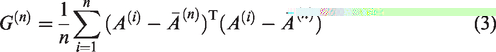
Suppose that there are n training samples in total, the ith training image is denoted by a matrix $A^{(i)}\in {ℝ}^{p\times q}$ where $i=1,2,\dots ,n$ . The empirical covariance matrix of image training samples set can be constructed by

$$G^{(n)}=\frac{1}{n}{\displaystyle \sum _{i=1}^n{(A^{(i)}-{\overline{A}}^{(n)})}^{\text{T}}}(A^{(i)}-{\overline{A}}^{(n)})$$

(3)

where ${\overline{A}}^{(n)}=\frac{1}{n}{\displaystyle {\sum }_{i=1}^n{A}^{(i)}}$ is the mean of the image training samples. Let $y^{(n)}\in {ℝ}^q$ with $\left|\right|y^{(n)}|{|}_2=1$ . The generalized total scatter criterion is defined as

$$J(y^{(n)})={(y^{(n)})}^{\text{T}}{G}^{(n)}{y}^{(n)}$$

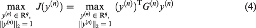
In fact, $J(y^{(n)})$ is the Rayleigh quotient of the covariance matrix on the projection vector $y^{(n)}$ . ³³ Then, the 2DPCA algorithm finds an optimal projection vector such that it maximizes

$$\underset{\hspace{0.17em}}{\underset{\begin{array}{c}{y}^{(n)}\in {ℝ}^q,\\ \left|\right|y^{(n)}|{|}_2=1\end{array}}{\max }}J(y^{(n)})=\underset{\hspace{0.17em}}{\underset{\begin{array}{c}{y}^{(n)}\in {ℝ}^q,\\ \left|\right|y^{(n)}|{|}_2=1\end{array}}{\max }}{(y^{(n)})}^{\text{T}}{G}^{(n)}{y}^{(n)}$$

(4)

Usually, only one optimal projection vector is not enough. When a set of projection vectors $\{y_1^{(n)},\dots ,y_k^{(n)}\}$ are needed where k < q, then $y_i^{(n)}$ for $i=2,\dots ,k$ can be obtained sequentially by maximizing $J(y_i^{(n)})$ subject to additional orthogonality constraints, i.e., $y_i^{(n)}$ required orthogonality against those vectors that are already computed. It is equivalent to solve the following optimization problem

$$\begin{array}{l}\underset{\hspace{0.17em}}{\underset{Y^{(n)}\in {ℝ}^{q\times k}}{\max }}\text{tr}\left({(Y^{(n)})}^{\text{T}}{G}^{(n)}{Y}^{(n)}\right)\\ \text{s}.\text{t}.{(Y^{(n)})}^{\text{T}}{Y}^{(n)}{\mathit{=I}}_k\end{array}$$

(5)

where $Y^{(n)}=[y_1^{(n)},\dots ,y_k^{(n)}]\in {ℝ}^{q\times k}$ . In general, the solution of (5) can be obtained by computing the eigenvalue decomposition of $G^{(n)}$ . Denote by ${\lambda }_i^{(n)}$ the eigenvalues of $G^{(n)}$ and order them as

$${\lambda }_1^{(n)}\ge {\lambda }_2^{(n)}\ge \cdots \ge {\lambda }_q^{(n)}$$

(6)

Then, $y_1^{(n)},\dots ,y_k^{(n)}$ are the eigenvectors corresponding to ${\lambda }_1^{(n)},\dots ,{\lambda }_k^{(n)}$ , i.e.

$$G^{(n)}{Y}^{(n)}=Y^{(n)}{\Lambda }^{(n)}\text{and}{(Y^{(n)})}^{\text{T}}{Y}^{(n)}=I_k$$

(7)

where ${\Lambda }^{(n)}=\text{diag}({\lambda }_1^{(n)},\dots ,{\lambda }_k^{(n)})$ .

The traditional 2DPCA algorithm is an offline learning algorithm, and it is also referred to as the batch 2DPCA algorithm. The reason is that it needs to acquire all the training samples information in advance. As new image training samples are input, the batch 2DPCA algorithm (5) usually discards the training acquisition in the past, and then recomputes the covariance matrix and the wanted eigenpairs by using all currently available training samples. When the number of training samples is large, the storing and calculating of recomputing the eigenvalue decomposition for newly added data are both very expensive. To tackle the above limitations, analogously to CCIPCA, ²¹ the I2DPCA algorithm is developed in Ge et al. ²³ as follows.

Let $A^{(n)}\in {ℝ}^{p\times q}$ be a newly added image training sample. Then, the overall mean is calculated by

$${\overline{A}}^{(n)}=\frac{n-1}{n}{\overline{A}}^{(n-1)}+\frac{1}{n}{A}^{(n)}$$

(8)

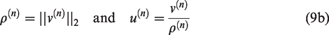
and the computed eigenvalue and the associated eigenvector are updated as

$$v^{(n)}=\frac{n-1-\ell }{n}{v}^{(n-1)}+\frac{1+\ell }{n}{({\widehat{A}}^{(n)})}^{\text{T}}{\widehat{A}}^{(n)}\frac{v^{(n-1)}}{\left|\right|v^{(n-1)}|{|}_2}$$

(9a)

$${\rho }^{(n)}=\left|\right|v^{(n)}|{|}_2\text{and}{u}^{(n)}=\frac{v^{(n)}}{{\rho }^{(n)}}$$

(9b)

where ${\widehat{A}}^{(n)}=A^{(n)}-{\overline{A}}^{(n)}$ and $\ell$ denotes the amnesic parameter with its range from 2 to 4. In (9 b), ${\rho }^{(n)}$ and $u^{(n)}$ are the estimations of the largest eigenvalue ${\lambda }_1^{(n)}$ and the corresponding eigenvector $y_1^{(n)}$ , respectively. To compute the other eigenvectors $y_{j+1}^{(n)}$ for $j\ge 1$ , the centered sample matrices must be subtracted from its projection on the estimated jth order eigenvector $u_j^{(n)}$ as (2), i.e.

$${\widehat{A}}_{j+1}^{(n)}={\widehat{A}}_j^{(n)}-{\widehat{A}}_j^{(n)}{u}_j^{(n)}{(u_j^{(n)})}^{\text{T}}$$

(10)

where ${\widehat{A}}_1^{(n)}={\widehat{A}}^{(n)}$ and $u_1^{(n)}=u^{(n)}$ . Then, as (9), we use

$$v_{j+1}^{(n)}=\frac{n-1-\ell }{n}{v}_{j+1}^{(n-1)}+\frac{1+\ell }{n}{({\widehat{A}}_{j+1}^{(n)})}^{\text{T}}{\widehat{A}}_{j+1}^{(n)}\frac{v_{j+1}^{(n-1)}}{\left|\right|v_{j+1}^{(n-1)}|{|}_2}$$

(11a)

$${\rho }_{j+1}^{(n)}=\left|\right|v_{j+1}^{(n)}|{|}_2\text{and}{u}_{j+1}^{(n)}=\frac{v_{j+1}^{(n)}}{{\rho }_{j+1}^{(n)}}$$

(11b)

to obtain $u_{j+1}^{(n)}$ approximating to $y_{j+1}^{(n)}$ . Here, though ${\widehat{A}}_{j+1}^{(n)}{u}_j^{(n)}=0$ by (10), it is clear that

$${(u_j^{(n)})}^{\text{T}}{u}_{j+1}^{(n)}=\frac{n-1-\ell }{n{\rho }_{j+1}^{(n)}}{(u_j^{(n)})}^{\text{T}}{v}_{j+1}^{(n-1)}$$

(12)

is usually not equal to zero. It leads that the computed eigenvectors are not orthogonal each other, which will be detailed in our numerical examples. One can orthogonalize the approximate eigenvectors by the Gram-Schmidt orthogonalization ³³ as a post-processing step of (11), but it needs to add extra computational cost and the calculated result in such way is generally not the optimal approximation of (5). ³⁰

The subspace type I2DPCA algorithm

To solve the problem mentioned at the end of previous section, in this section, we present a subspace type algorithm for I2DPCA when more than one eigenvectors are required. Our motivation is from early work on the incremental principal component analysis given by Oja and Karhunen, ³⁴ where they introduced a subspace type extension of the stochastic gradient ascent algorithm (SGA) algorithm. We denote it by the SSGA algorithm which is given by

$$V^{(n)}=U^{(n-1)}+{\beta }^{(n-1)}{X}_{(:,j)}{X}_{(:,j)}^{\text{T}}{U}^{(n-1)}$$

(13a)

$$U^{(n)}=V^{(n)}{P}^{(n)}$$

(13b)

where $P^{(n)}$ is a normalization matrix to make $U^{(n)}$ have orthonormal columns. The nearly optimal convergence rate for the iteration (13) is proved in the recent paper. ³⁵ It is natural to generalize the SSGA algorithm for 2 D sample image matrices as

$$V^{(n)}=U^{(n-1)}+{\beta }^{(n-1)}{({\widehat{A}}^{(n)})}^{\text{T}}{\widehat{A}}^{(n)}{U}^{(n-1)}$$

(14a)

$$U^{(n)}=V^{(n)}{P}^{(n)}$$

(14b)

where $U^{(n-1)}\in {ℝ}^{q\times k}$ , and such a $P^{(n)}\in {ℝ}^{k\times k}$ is chosen as $P^{(n)}={[{(V^{(n)})}^{\text{T}}{V}^{(n)}]}^{-1/2}$ in literature.^34,35

In the above process, notice that $U^{(n-1)}$ in the right-hand side of the iteration (14a) is normalized, i.e., ${(U^{(n-1)})}^{\text{T}}{U}^{(n-1)}=I_k$ , but the second term can take any magnitude which depends on the magnitude of the 2 D sample image matrix $A^{(n)}$ . In case $A^{(n)}$ is a very small magnitude, the second term will be too small to make any updating in the new estimation of $V^{(n)}$ . If $A^{(n)}$ has a large magnitude, the second term will dominate the right-hand side of (14a). Hence, similar to Weng et al., ²¹ to balance the role of the first and second terms, we derive our subspace type I2DPCA algorithm from the eigenvalue decomposition of $G^{(n)}$ . Using the notations of the previous section, let $Z^{(n)}=Y^{(n)}{\Lambda }^{(n)}$ and write $Y^{(n)}=U^{(n-1)}+\Delta Y^{(n-1)}$ . Suppose that $U^{(n-1)}$ is equal to $Y^{(n-1)}$ , i.e., $G^{(n-1)}{U}^{(n-1)}=U^{(n-1)}{\Lambda }^{(n-1)}$ . Then, according to the definition of eigenvalue decomposition, we have

$$\begin{array}{l}{Z}^{(n)}=Y^{(n)}{\Lambda }^{(n)}=G^{(n)}{Y}^{(n)}=\frac{1}{n}{\displaystyle \sum _{i=1}^n{({\widehat{A}}^{(i)})}^{\text{T}}}{\widehat{A}}^{(i)}{Y}^{(n)}\\ =\frac{1}{n}{\displaystyle \sum _{i=1}^{n-1}{({\widehat{A}}^{(i)})}^{\text{T}}}{\widehat{A}}^{(i)}{Y}^{(n)}+\frac{1}{n}{({\widehat{A}}^{(n)})}^{\text{T}}{\widehat{A}}^{(n)}{Y}^{(n)}\\ =\frac{n-1}{n}\frac{1}{n-1}{\displaystyle \sum _{i=1}^{n-1}{({\widehat{A}}^{(i)})}^{\text{T}}}{\widehat{A}}^{(i)}{Y}^{(n)}+\frac{1}{n}{({\widehat{A}}^{(n)})}^{\text{T}}{\widehat{A}}^{(n)}{Y}^{(n)}\\ =\frac{n-1}{n}{G}^{(n-1)}{Y}^{(n)}+\frac{1}{n}{({\widehat{A}}^{(n)})}^{\text{T}}{\widehat{A}}^{(n)}{Y}^{(n)}\\ =\frac{n-1}{n}{G}^{(n-1)}(U^{(n-1)}+\Delta Y^{(n-1)})\\ +\frac{1}{n}{({\widehat{A}}^{(n)})}^{\text{T}}{\widehat{A}}^{(n)}(U^{(n-1)}+\Delta Y^{(n-1)})\\ =\frac{n-1}{n}{G}^{(n-1)}{U}^{(n-1)}+\frac{1}{n}{({\widehat{A}}^{(n)})}^{\text{T}}{\widehat{A}}^{(n)}{U}^{(n-1)}\\ +G^{(n)}\Delta Y^{(n-1)}\\ =\frac{n-1}{n}{U}^{(n-1)}{\Lambda }^{(n-1)}+\frac{1}{n}{({\widehat{A}}^{(n)})}^{\text{T}}{\widehat{A}}^{(n)}{U}^{(n-1)}\\ +G^{(n)}\Delta Y^{(n-1)}\end{array}$$

(15)

As the process of iterations, it naturally hopes that the approximation is gradually close to $Y^{(n)}$ , i.e., $\Delta Y^{(n-1)}$ having a tiny magnitude. Therefore, by simply regarding $\Delta Y^{(n-1)}$ as 0, we apply the iteration

$$V^{(n)}=\frac{n-1}{n}{U}^{(n-1)}{\Lambda }^{(n-1)}+\frac{1}{n}{({\widehat{A}}^{(n)})}^{\text{T}}{\widehat{A}}^{(n)}{U}^{(n-1)}$$

(16)

to approximate $Z^{(n)}$ .

Next, to establish the relationship between $V^{(n)}$ and $Y^{(n)}$ , let the eigenvalue decomposition of $G^{(n)}$ be

$$\begin{array}{l}{G}^{(n)}=[Y^{(n)},Y_{\perp }^{(n)}]\left[\begin{array}{ll}{\Lambda }^{(n)}& 0\\ 0& {\Lambda }_{\perp }^{(n)}\end{array}\right]\left[\begin{array}{l}{(Y^{(n)})}^{\text{T}}\\ {(Y_{\perp }^{(n)})}^{\text{T}}\end{array}\right]\\ =Y^{(n)}{\Lambda }^{(n)}{(Y^{(n)})}^{\text{T}}+Y_{\perp }^{(n)}{\Lambda }_{\perp }^{(n)}{(Y_{\perp }^{(n)})}^{\text{T}}\end{array}$$

(17)

where $[Y^{(n)},Y_{\perp }^{(n)}]$ is a q × q orthonormal matrix. By (16), it follows that

$$\begin{array}{l}{V}^{(n)}=\frac{n-1}{n}{G}^{(n-1)}{U}^{(n-1)}+\frac{1}{n}{({\widehat{A}}^{(n)})}^{\text{T}}{\widehat{A}}^{(n)}{U}^{(n-1)}\\ =G^{(n)}{U}^{(n-1)}=G^{(n)}(Y^{(n)}-\Delta Y^{(n-1)})\\ =Y^{(n)}{\Lambda }^{(n)}{(Y^{(n)})}^{\text{T}}{Y}^{(n)}+Y_{\perp }^{(n)}{\Lambda }_{\perp }^{(n)}{(Y_{\perp }^{(n)})}^{\text{T}}{Y}^{(n)}\\ -G^{(n)}\Delta Y^{(n-1)}\\ =Y^{(n)}{\Lambda }^{(n)}-Y^{(n)}{\Lambda }^{(n)}{(Y^{(n)})}^{\text{T}}\Delta Y^{(n-1)}\\ -Y_{\perp }^{(n)}{\Lambda }_{\perp }^{(n)}{(Y_{\perp }^{(n)})}^{\text{T}}\Delta Y^{(n-1)}\\ =Y^{(n)}{\Lambda }^{(n)}\left(I-{(Y_{\perp }^{(n)})}^{\text{T}}\Delta Y^{(n-1)}\right)\\ -Y_{\perp }^{(n)}{\Lambda }_{\perp }^{(n)}{(Y_{\perp }^{(n)})}^{\text{T}}\Delta Y^{(n-1)}\\ \approx Y^{(n)}{D}^{(n)}\end{array}$$

(18)

where $D^{(n)}={\Lambda }^{(n)}(I-{(Y_{\perp }^{(n)})}^{\text{T}}\Delta Y^{(n-1)}$ ). That means the approximation of $Y^{(n)}$ can be obtained by orthogonalizing the columns of $V^{(n)}$ . Though several ways can be used to realize the purpose, such as ${[{(V^{(n)})}^{\text{T}}{V}^{(n)}]}^{-1/2}$ , we prefer the QR factorization of $V^{(n)}$ . The reason is that compared to ${[{(V^{(n)})}^{\text{T}}{V}^{(n)}]}^{-1/2}$ , the QR decomposition needs less computation cost and performs better numerical stability. Let the QR decomposition of $V^{(n)}$ be $V^{(n)}=U^{(n)}{R}^{(n)}$ where $U^{(n)}$ and $R^{(n)}$ are the Q-factor and R-factor of $V^{(n)}$ , respectively. Then, $U^{(n)}$ will be an approximation of $Y^{(n)}$ .

In addition, it is noted that ${\Lambda }^{(n-1)}$ is unknown in (16). As the definition of $D^{(n)}$ in (18), the matrix $D^{(n-1)}$ can be considered as the perturbation of ${\Lambda }^{(n-1)}$ with a multiplication structure, ³⁶ and its diagonal elements are very close to the diagonal entries of ${\Lambda }^{(n-1)}$ when $\Delta Y^{(n-2)}$ has a tiny magnitude. Based on the QR decomposition $V^{(n-1)}=U^{(n-1)}{R}^{(n-1)}$ , it is natural to use the diagonal elements of $R^{(n-1)}$ as estimations of the eigenvalues. Therefore, our incremental iteration can be written as

$$V^{(n)}=\frac{n-1}{n}{\tilde{U}}^{(n-1)}+\frac{1}{n}{({\widehat{A}}^{(n)})}^{\text{T}}{\widehat{A}}^{(n)}{U}^{(n-1)}$$

(19a)

$$U^{(n)}{R}^{(n)}=V^{(n)}\text{and}{\tilde{U}}^{(n)}=U^{(n)}{R}_D^{(n)}$$

(19b)

where $R_D^{(n)}=\text{diag}(R_{(1:1)}^{(n)},\dots ,R_{(k:k)}^{(n)})$ and ${\tilde{U}}^{(n-1)}=U^{(n-1)}{R}_D^{(n-1)}$ . Compared to the SSGA algorithm (14), $(n-1)/n$ and $1/n$ are the weights for the last estimate and the new data here, respectively, and ${\tilde{U}}^{(n-1)}$ is without normalization though it has orthogonal columns.

We summarize what we have done in this section in Algorithm 1, i.e., the subspace type incremental 2 D principal component analysis algorithm. We denote it by SI2DPCA for convenience. Finally, a few remarks regarding Algorithm 1 are in order:

The initial matrices $U^{(0)},{\tilde{U}}^{(0)}$ and ${\overline{A}}^{(0)}$ in Algorithm 1 are from the initial learning system which contains n₀ samples. Let its empirical covariance matrix be $G^{(0)}$ . Then, ${\overline{A}}^{(0)}$ is the mean of these n₀ sample matrices, and we set $U^{(0)}$ and ${\tilde{U}}^{(0)}$ satisfying $G^{(0)}{U}^{(0)}=U^{(0)}{\Lambda }^{(0)},{(U^{(0)})}^{\text{T}}{U}^{(0)}=I_k$ and ${\tilde{U}}^{(0)}=U^{(0)}{\Lambda }^{(0)}$ where ${\Lambda }^{(0)}=\text{diag}({\lambda }_1^{(0)},\dots ,{\lambda }_k^{(0)})$ with ${\lambda }_1^{(0)},\dots ,{\lambda }_k^{(0)}$ being the first k largest eigenvalues of $G^{(0)}$ .

As (9a), to speed up the convergence of the estimation, the amnesic parameter $\ell$ is also applied at step 5 of Algorithm 1 to give a larger weight for new samples. Typically, $\ell$ is from 2 to 4. In our numerical example, we just simply take $\ell =2$ .

At step 6, to compute the QR decomposition of $V^{(i)}$ with economy-size, we use the MATLAB built-in function qr( $V^{(i)}$ ,0) to obtain the matrices $U^{(i)}$ and $R^{(i)}$ where $U^{(i)}\in {ℝ}^{q\times k}$ with ${(U^{(i)})}^{\text{T}}{U}^{(i)}=I_k$ and $R^{(i)}$ is a k × k upper triangular matrix.

Compared to the single-vector I2DPCA algorithm (11), Algorithm 1 does not need to correct the sample matrices when several eigenvectors are required, and the approximate eigenvectors extracted from the QR decomposition to make sure the orthogonality, i.e., ${(U^{(i)})}^{\text{T}}{U}^{(i)}=I_k$ always holds in Algorithm 1. Additionally, Algorithm 1 due to its ability in updating all approximate eigenvectors of interest at the same time is looked forward to lower time cost.

Algorithm 1. The subspace type I2DPCA algorithm (SI2DPCA).

Input: Initialization $U^{(0)},{\tilde{U}}^{(0)},{\overline{A}}^{(0)}$ and n₀, and newly added 2 D sample image matrices $A^{(1)},A^{(2)},\dots ,A^{(n)}$ .

Output: The matrix composed of the first k orthogonal eigenvectors.

1: for $i=1,2,\dots ,n$ , the following steps do

2:  $m=n_0+i$ ,

3:  ${\overline{A}}^{(i)}=\frac{m-1}{m}{\overline{A}}^{(i-1)}+\frac{1}{m}{A}^{(i)}$ ,

4:  ${\widehat{A}}^{(i)}=A^{(i)}-{\overline{A}}^{(i)}$ ,

5:  $V^{(i)}=\frac{m-1-\ell }{m}{\tilde{U}}^{(i-1)}+\frac{1+\ell }{m}{({\widehat{A}}^{(i)})}^{\text{T}}{\widehat{A}}^{(i)}{U}^{(i-1)}$ ,

6: compute the QR factorization of $V^{(i)}$ to get $U^{(i)}$ and $R^{(i)}$ ,

7: let $R_D^{(i)}=\text{diag}(R_{(1:1)}^{(i)},\dots ,R_{(k:k)}^{(i)})$ and ${\tilde{U}}^{(i)}=U^{(i)}{R}_D^{(i)}$ .

8: end for

Numerical example

To demonstrate the effectiveness and efficiency of our proposed SI2DPCA algorithm, we compare it with the I2DPCA ²³ and SSGA (14) algorithms on some publicly available datasets. Our goal is to compute the first 8 principal component vectors, i.e., $y_j^{(n)}$ for $1\le j\le 8$ . We select the parameters ${\beta }^{(n-1)}=1/n$ in SSGA (14) as Weng et al. ²¹ In demonstrating the quality and orthogonality of computed approximations, we calculate the cosine of acute angles ${\theta }_j^{(i)}$ between $u_j^{(i)}$ and $y_j^{(n)}$

$$\cos {\theta }_j^{(i)}=\frac{\left|{(u_j^{(i)})}^{\text{T}}{y}_j^{(n)}\right|}{{\left|\left|u_j^{(i)}\right|\right|}_2{\left|\left|y_j^{(n)}\right|\right|}_2}$$

(20)

and the orthogonality errors ${\eta }^{(i)}$ and ${\epsilon }^{(i)}$ defined by

$${\eta }^{(i)}=\left|{(u_1^{(i)})}^{\text{T}}{u}_2^{(i)}\right|,{\epsilon }^{(i)}={\left|\left|{(U^{(i)})}^{\text{T}}{U}^{(i)}-I_k\right|\right|}_{\text{F}}$$

(21)

where $y_j^{(n)}$ are computed by the batch 2DPCA algorithm with MATLAB’s function eig on $G^{(n)}$ , which are considered to be the “exact” eigenvalues for test purposes, and $u_j^{(i)}=U_{(:,j)}^{(i)}$ in Algorithm 1. The orthogonality errors ${\eta }^{(i)}$ and ${\epsilon }^{(i)}$ monitor the orthogonality between $u_1^{(i)}$ and $u_2^{(i)}$ , and the columns of $U^{(i)}$ , respectively. It is noted that

$${\eta }^{(i)}\le {\left|\left|u_1^{(i)}\right|\right|}_2{\left|\left|u_2^{(i)}\right|\right|}_2\le 1$$

(22)

All the experiments in this paper are executed on a Windows 10 (64 bit) Laptop-Intel(R) Core(TM) i5-4210U CPU 1.70 GHz, 4 GB of RAM using MATLAB 2018a with machine epsilon $2.22\times {10}^{-16}$ in double-precision floating-point arithmetic. Each random experiment is repeated 10 times independently, then the average numerical results are reported.

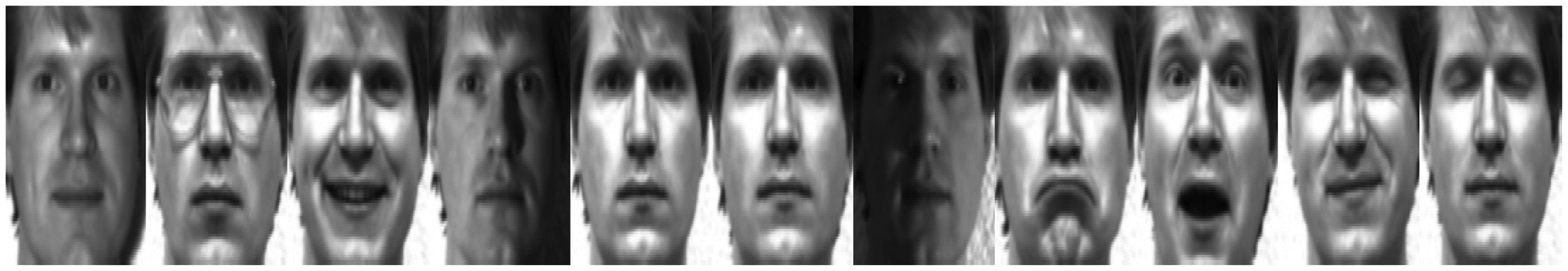
Example 1 (Experiments on the FERET dataset). The FERET dataset (http://www.nist.gov/itl/iad/ig/colorferet.cfm) is a large face image dataset for face recognition. There are 1400 images of 200 individuals (71 females and 129 males), including frontal views of faces with different facial expressions, lighting conditions, and photographing angle. We manually crop the face portion of the image and then normalized it with the same resolution of 80 × 80 pixels. The normalized images of one individual are shown in Figure 1.

Figure 1.

Seven images of one person from the FERET dataset.

In this example, one sample is selected randomly from the entire database as the initial learning system, and remaining samples are applied for testing incremental algorithms. We compare the accuracy of computed approximations $\cos {\theta }_j^{(i)}$ and orthogonality errors defined in (20) and (21), respectively, the CPU time in seconds, and the image reconstruction for the SSGA, I2DPCA, and SI2DPCA algorithms in the FERET dataset. Figure 2 presents the convergence behavior of SSGA, I2DPCA and SI2DPCA for computing the first 8 eigenvectors. To the best of our knowledge, if $\cos {\theta }_j^{(i)}$ trends to 1, it means incremental methods have good agreement with batch methods, but the corresponding cosine values of the SSGA algorithm fluctuate dramatically, and the largest one is not higher than 75%. A similar phenomenon also appears in the single-vector version of SGA. ²¹ In addition, in Figure 2, it is not difficult to find that I2DPCA and SI2DPCA have better accuracy than SSGA. With the increasing number of samples, $\cos {\theta }_j^{(i)}$ of the first 8 approximate eigenvectors of the I2DPCA and SI2DPCA algorithms gradually are close to or reach 1. However, the quality of the computed approximations of SI2DPCA still outperforms than I2DPCA.

Figure 2.

Convergence behavior of SSGA, I2DPCA and SI2DPCA with the first four eigenvectors and the later four ones, respectively.

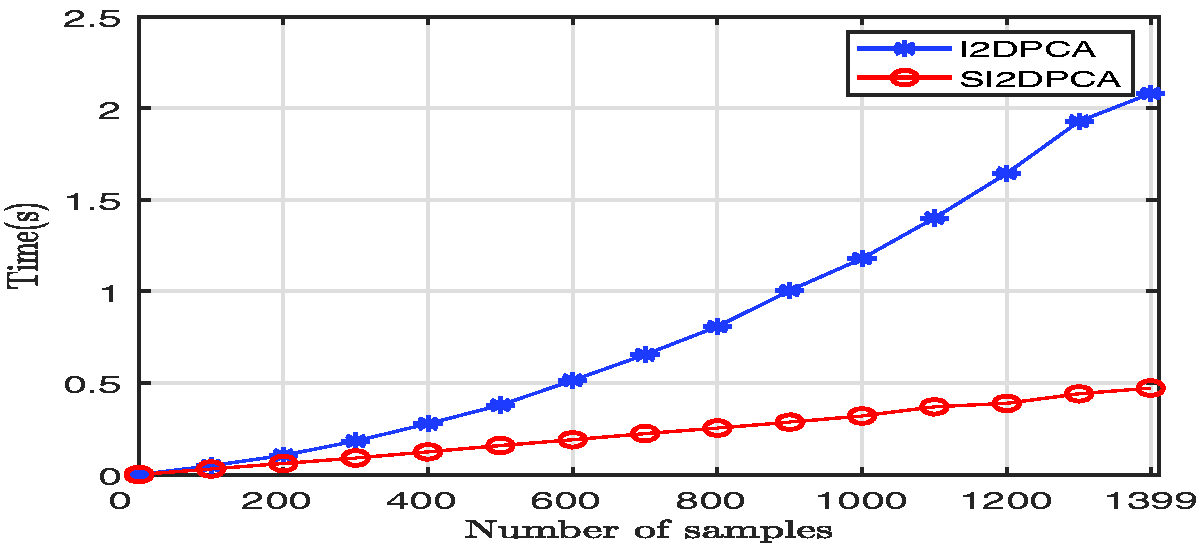
Notice that SSGA and SI2DPCA are both subspace type algorithms. It leads to that the SSGA algorithm performs almost the same numerical results in orthogonality errors and CPU time as SI2DPCA, which are not collected in our numerical examples. Therefore, in what follows, we only discuss the orthogonality errors and CPU time for SI2DPCA and I2DPCA algorithms, which are reported in Figures 3 and 4, respectively. It is demonstrated by Figure 3 that the orthogonality errors ${\eta }^{(i)}$ and ${\epsilon }^{(i)}$ of SI2DPCA are held around ${10}^{-15}$ , which is near to the double-precision of floating-point arithmetic, while those of I2DPCA are close to ${10}^{-1}$ except the first one coming from the initial system. That means the loss of orthogonality constraints on the extracted eigenvectors in the equation (5) has happened in the first iteration of I2DPCA for calculating the second-order eigenvector, but the SI2DPCA algorithm always keeps the orthogonality very well, which indicates that extracted principal component vectors are mutually uncorrelated. Computational time with respect to the number of samples is presented in Figure 4. It is observed that, compared to I2DPCA, the SI2DPCA algorithm reduces remarkably the computational time. Specifically, in Figure 4, when the number of samples is increased, SI2DPCA has a more obvious advantage in terms of the CPU time than I2DPCA. That means if the larger the sample size is referred, the difference in the CPU time will be more dramatic.

Figure 3.

Orthogonality errors ${\eta }^{(i)}$ (left) and ${\epsilon }^{(i)}$ (right) of I2DPCA and SI2DPCA.

Figure 4.

Comparison of the required CPU time in seconds for I2DPCA and SI2DPCA under the increasing of samples.

In this example, we also consider the reconstructed image of sample $A^{(i)}$ based on the computed eigenvectors. It is noted $[Y^{(n)},Y_{\perp }^{(n)}]$ is orthonormal in the eigen-decomposition of $G^{(n)}$ (17). Thus

$$\begin{array}{l}{A}^{(i)}=A^{(i)}[Y^{(n)},Y_{\perp }^{(n)}]\left[\begin{array}{l}{(Y^{(n)})}^{\text{T}}\\ {(Y_{\perp }^{(n)})}^{\text{T}}\end{array}\right]\\ =A^{(i)}{Y}^{(n)}{(Y^{(n)})}^{\text{T}}+A^{(i)}{Y}_{\perp }^{(n)}{(Y_{\perp }^{(n)})}^{\text{T}}\end{array}$$

(23)

As stated in Yang et al., ¹⁵ $A_k^{(i)}=A^{(i)}{Y}^{(n)}{(Y^{(n)})}^{\text{T}}$ is of the same size as the sample $A^{(i)}$ and represents the reconstructed image of $A^{(i)}$ . Usually, the exact $Y^{(n)}$ is not available. It is natural that we use the computed approximations $U^{(n)}$ to replace with $Y^{(n)}$ to get ${\tilde{A}}_k^{(i)}=A^{(i)}{U}^{(n)}{(U^{(n)})}^{\text{T}}$ . Figure 5 shows the reconstructed images ${\tilde{A}}_k^{(i)}$ with k from 1 to 8. It is exhibited that the reconstructed images become clearer with the number of eigenvectors is increased. Notice that, when k = 8, the image reconstructed by our method has a change in the mouth, which is similar to the original image appearing in the last image of Figure 1, while that of I2DPCA is still the same as k = 7 in this example.

Figure 5.

Reconstructed images based on I2DPCA (upper) and SI2DPCA (lower) with k varying from 1 to 8.

Example 2 (Experiments on the Yale Dataset). Face-image variations in the Yale dataset (https://computervisiononline.com/dataset/1105138686) include illumination (left-light, center-light, and right-light), facial expression (normal, happy, sad, sleepy, surprised, and a wink) and with or without glasses. In our experiment, 15 individuals with 165 images are selected. All images are grayscale and normalized with resolution 100 × 100 pixels. We show eleven images of one individual from the Yale dataset in Figure 6.

Figure 6.

Eleven images of one person from the Yale dataset.

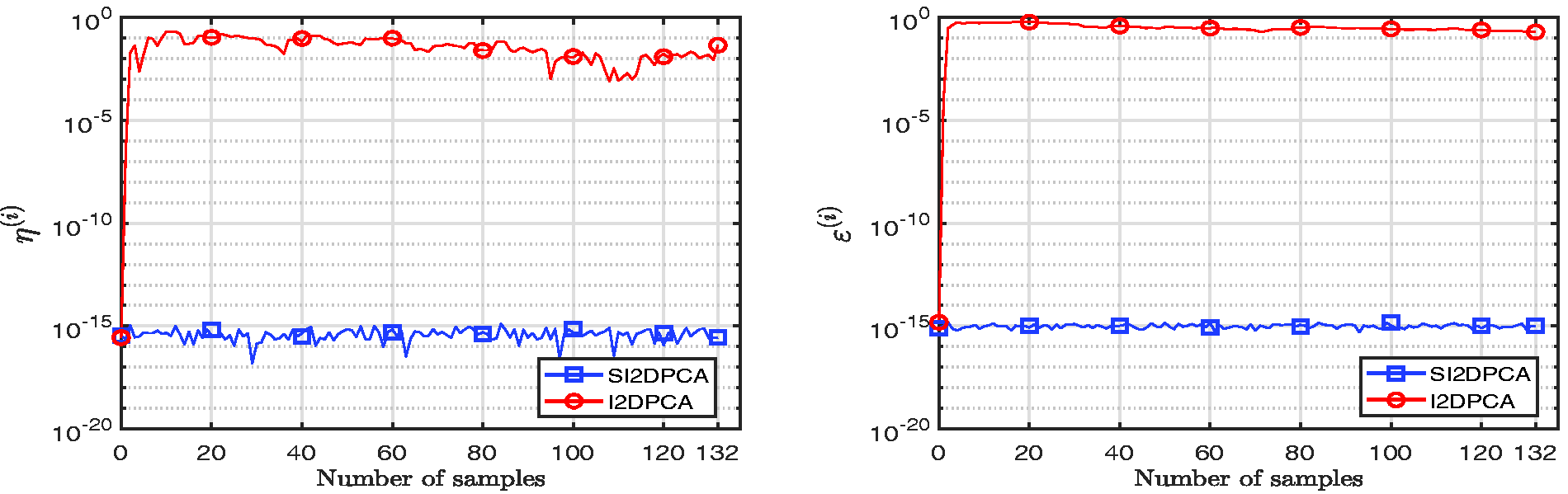
We randomly choose 20% samples for the initial system, and the rest samples are used for incremental learning, i.e., 33 and 132 image samples, respectively. The accuracy of computed approximations $\cos {\theta }_j^{(i)}$ , and orthogonality errors ${\eta }^{(i)}$ and ${\epsilon }^{(i)}$ are plotted in Figures 7 and 8, respectively. They exhibit similar numerical behavior as Figures 2 and 3. In particular, in such a case, the SSGA algorithm is still not convergence by Figure 7, and all approximated eigenvectors computed by SI2DPCA are all close enough to 1, which performs superior to I2DPCA on the accuracy of computed approximations. From Figure 8, we observe that the calculated approximated eigenvectors by I2DPCA are not mutually orthogonal as well in this example, since their orthogonality errors ${\eta }^{(i)}$ and ${\epsilon }^{(i)}$ go from $3\times {10}^{-1}$ to 1, while orthogonality errors ${\eta }^{(i)}$ and ${\epsilon }^{(i)}$ of SI2DPCA are always between ${10}^{-16}$ and ${10}^{-15}$ .

Figure 7.

Convergence behavior of SSGA, I2DPCA and SI2DPCA for computing the first 8 eigenvectors.

Figure 8.

Orthogonality errors ${\eta }^{(i)}$ (left) and ${\epsilon }^{(i)}$ (right) of I2DPCA and SI2DPCA.

For the required CPU time, as shown in Figure 9(a), we consider comparing the difference between the I2DPCA and SI2DPCA algorithms with the number of wanted eigenvectors from k = 1 to k = 8. It is demonstrated that, as the number of wanted eigenvectors increased, the computational time of SI2DPCA increases significantly, but the CPU time of SI2DPCA does not change obviously, which is mainly due to subspace type methods calculating the k eigenvectors at one time when a new sample is input. Additionally, when k = 8, we repeat the I2DPCA and SI2DPCA algorithms 50, 250, 500 and 1000 times, respectively, and collect the associated average execution time in Figure 9(b) to show the efficiency of SI2DPCA.

Figure 9.

Comparison of the required CPU time in seconds for I2DPCA and SI2DPCA with increasing the number of wanted eigenvectors (a) and the average execution time with different times of repetition (b).

Example 3 (Experiments on the ORL, AR, PIE and JAFFE Dataset). The ORL dataset (https://www.cl.cam.ac.uk/research/dtg/attarchive/facedatabase.html) contains 400 face images of 40 distinct persons. The size of ORL images is 92 × 112 pixels with 256 gray levels. The images are collected by volunteers at different times, different lighting, different facial expressions (blinking or closed eyes, smiling or no-smiling), and facial details (wearing glasses or no-glasses). Ten example images of one person from the ORL dataset are shown in Figure 10.

Figure 10.

Ten images of one person from the ORL dataset.

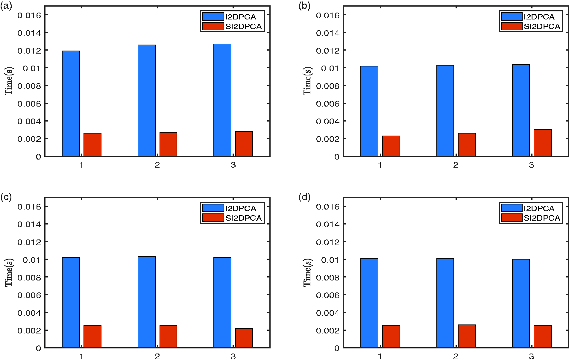
We take the five image samples selected randomly from all samples as “old” samples for exact calculations, and remaining samples are for incremental methods. Numerical results in Figures 11 and 12 clearly show that SI2DPCA outperforms significantly in the computational approximations and orthogonality in this example. As in Han et al., ³⁷ we consider the required CPU time in seconds of newly added samples based on the initial train sample number being 285, 315, 335 and 355, respectively. The number of newly added samples is set to 15 each time, and the numerical results of new samples added 3 times are recorded in Figure 13. It is not difficult to find that the incremental learning time of I2DPCA and SI2DPCA is almost unchanged in such a case. Regardless of the size of the initial training set, the SI2DPCA algorithm always reduces remarkably the computational time.

Figure 11.

Convergence behavior of SSGA, I2DPCA and SI2DPCA for calculating the first 8 eigenvectors.

Figure 12.

Orthogonality errors ${\eta }^{(i)}$ (left) and ${\epsilon }^{(i)}$ (right) of I2DPCA and SI2DPCA.

Figure 13.

Computational time of I2DPCA and SI2DPCA added 15 samples each time with the number of initial training sets being 285 (a), 315 (b), 335 (c) and 355 (d), respectively.

In this example, we also make a summary comparison of SSGA, I2DPCA, and SI2DPCA based on the datasets appeared in Table 1, i.e., AR (http://rvl1.ecn.purdue.edu/ aleix/aleix_face_DB.html), PIE (http://www.flintbox.com/public/project/4742/) and JAFFE, ³⁸ which also details the number of row and column of image matrices p and q, respectively, and the number of image samples n of these three datasets. The average of $\sin {\theta }_j^{(n)}$ for $j=1,\dots ,8$ where ${\theta }_j^{(i)}$ is defined in (20), together with ${\eta }^{(n)},{\epsilon }^{(n)}$ and CPU time in seconds are collected in Table 2. Similar comments we made at Examples 1 and 2 are still valid here as well.

Table 1.

The detail of AR, PIE and JAFFE datasets.

Problems	AR dataset	PIE dataset	JAFFE
Size of image matrices p × q	40 × 40	64 × 64	256 × 256
Number of image samples n	2600	1632	214

Table 2.

Comparison of SSGA, I2DPCA and SI2DPCA based on AR, PIE and JAFFE datasets.

Experiments	$\sin {\theta }_j^{(n)}(1\le j\le 8)$	${\epsilon }^{(n)}$	${\eta }^{(n)}$	CPU time (s)
AR dataset
SSGA	0.9206	$4.5042\times {10}^{-13}$	$1.3309\times {10}^{-13}$	0.2804
I2DPCA	0.3050	0.1182	0.0038	0.3499
SI2DPCA	0.1635	$1.0176\times {10}^{-15}$	$6.7931\times {10}^{-16}$	0.0927
PIE dataset
SSGA	0.9544	$2.963\times {10}^{-12}$	$4.2186\times {10}^{-13}$	0.2962
I2DPCA	0.3402	0.1349	0.0660	2.2273
SI2DPCA	0.0892	$9.7239\times {10}^{-16}$	$4.4816\times {10}^{-16}$	0.1729
JAFFE dataset
SSGA	0.9717	$1.0674\times {10}^{-13}$	$1.5359\times {10}^{-14}$	0.1818
I2DPCA	0.5038	0.2170	0.0067	2.3380
SI2DPCA	0.3903	$1.2225\times {10}^{-15}$	$6.6933\times {10}^{-16}$	0.1708

Conclusion

Like CCIPCA, ²¹ the essence of incremental two-dimensional PCA (I2DPCA) should be the incremental updating of one eigenvector at a time which leads to the non-orthogonality of the approximate eigenvectors. To remedy the problem, in this paper, we proposed a subspace type incremental 2DPCA algorithm (SI2DPCA), i.e., Algorithm 1, to incrementally update the eigenspace in a streaming environment. Thus, it can deal with volumes of additional data more efficiently.

To test the computational properties of SI2DPCA, we used SI2DPCA in a real-life streaming environment in which data are coming in the form of random. We conducted various tests on datasets with either the number of image samples n < 1000 (Yale, ORL and JAFFE datasets), or n > 1000 (FERET, AR and PIE dataset). We can summarize the advantages of SI2DPCA as follows: (1) SI2DPCA performs far superior to I2DPCA in terms of the accuracy of computed approximations; (2) SI2DPCA is able to effectively overcome the problem that the calculated eigenvectors are not mutually orthogonal in the existing I2DPCA algorithm; (3) SI2DPCA has very high memory and speed efficiency due to it can extract several eigenvectors in one-pass computation. These improvements will play a vital role in the processing streaming data analysis and online learning system of large datasets. Better numerical results in the computational approximations and orthogonality bring forth clearer reconstructed images, as shown in Figure 5.

From the point of view that the 2DPCA algorithm ¹⁵ can be considered as a one-directional 2DPCA algorithm, the developments of Algorithm 1 can be made to work for the bidirectional 2DPCA algorithm ² without much difficulty, but we do not detail this in this paper.