Sage Journals: Discover world-class research

Abstract

With the wide application of intelligent sensors and internet of things (IoT) in the smart job shop, a large number of real-time production data is collected. Accurate analysis of the collected data can help producers to make effective decisions. Compared with the traditional data processing methods, artificial intelligence, as the main big data analysis method, is more and more applied to the manufacturing industry. However, the ability of different AI models to process real-time data of smart job shop production is also different. Based on this, a real-time big data processing method for the job shop production process based on Long Short-Term Memory (LSTM) and Gate Recurrent Unit (GRU) is proposed. This method uses the historical production data extracted by the IoT job shop as the original data set, and after data preprocessing, uses the LSTM and GRU model to train and predict the real-time data of the job shop. Through the description and implementation of the model, it is compared with KNN, DT and traditional neural network model. The results show that in the real-time big data processing of production process, the performance of the LSTM and GRU models is superior to the traditional neural network, K nearest neighbor (KNN), decision tree (DT). When the performance is similar to LSTM, the training time of GRU is much lower than LSTM model.

Keywords

LSTM smart job shop big data deep learning

Introduction

Driven by industry 4.0,¹ the Internet of things (IoT)^2,3 technology is more and more widely used in industrial production. By virtue of RFID,⁴ embedded system,⁵ sensor network⁶ and software technology, the IoT realizes real-time monitoring of various production data of work in progress. Through the analysis of the collected production and manufacturing big data,⁷ the enterprise can complete the production task according to the plan. Industrial big data usually refers to a large amount of time-series data generated by industrial equipment in the factory at a high speed,⁸ which is more valuable than general big data. However, the current trend in industrial systems is to use different big data engines to process large amounts of data that cannot be processed by common infrastructure. Therefore, in recent years, more and more machine learning has been applied to solve the processing problem of big data in the smart job shop.^9,10

At present, big data technology has been applied to some specific production scenarios, such as scheduling, process optimization, fault tracking, process optimization, etc., most of them are machine learning, neural network, data mining, etc.¹¹ In the actual manufacturing process, most of the data collected by RFID is time series data,^12,13 which has a strong time correlation. Traditional machine learning and deep learning methods cannot effectively use the time correlation of data, while LSTM is widely used in machine translation, dialogue generation, coding and decoding technology, precisely because it is very suitable for dealing with the time series highly related problems. Therefore, this paper will take the forecast production plan as an example, establish the LSTM^14,15 and GRU^16,17 model to process the production process data, predict whether to reschedule the production plan, and help the production manager to complete the original production plan task on time.

The rest of this paper is arranged as follows. The second section reviews some research related to this study. The third section briefly introduces the LSTM and GRU models and their construction. The experimental and analysis results are shown in section ‘Experiment’. Finally, the conclusions and suggestions for future study are outlined.

Literature review

Traditional machine learning methods already have a lot of examples in the processing of big data in the production process. The traditional machine learning method has many examples in the processing of big data in the production process. For example, Tirkel et al. selected 19 features (wafer batch serial number, loading time, processing time, etc.) as the key indicators in the operation, and used decision tree and neural network model to predict the flow time in semiconductor manufacturing.¹⁸ Junliang Wang et al. proposed a big data analysis method. Firstly, the feature set was constructed, the dimension was reduced by the entropy-based feature selection method, and then a parallel cycle time forecasting model was used to predict the cycle time.¹⁹ In order to further improve the performance of the internal maturity of the Fab, the fuzzy C mean back propagation network method is combined with the nonlinear programming model to predict the completion time and cycle time.²⁰ However, due to the multicollinearity, high-dimensional feature space and timing of manufacturing data, the traditional shallow neural network model lacks the generalization and fitting ability to deal with manufacturing big data.²¹ Also, most of the previous studies need domain experts to extract features to reduce the input dimension, resulting in the final prediction results heavily dependent on engineering features.

As a major breakthrough in the field of artificial intelligence, deep learning has achieved far better performance than machine learning in many fields, such as voice, natural language, vision, etc. Through multi-layer cascading, deep learning can automatically carry out feature learning on high-dimensional data, so that experts in the field can no longer select features manually. For example, He M. et al. proposed a bearing fault diagnosis method based on deep learning, which used the optimized deep learning structure and neural network to diagnose bearing fault. It could accurately classify all kinds of bearing faults under different working conditions.²² Fang Weiguang et al. proposed a manufacturing execution remaining time prediction method based on deep learning to learn the representative characteristics from high-dimensional manufacturing big data, so as to achieve stable and accurate prediction of the remaining time.²³ However, these in-depth learning models do not take into account the time correlation of production process data. LSTM can automatically select how many historical data to use as the influencing factors of the current prediction results, make better use of the time correlation in production and manufacturing data, and extract more features from the original data for analysis.

Most of the data generated in the production process of smart job shop is time series data. The LSTM and GRU models have strong temporal and spatial correlation, which have great advantages in the processing of time series data. Therefore, this paper uses LSTM and GRU models to process the big data generated in the production process of smart job shop, and studies the performance of LSTM and GRU models.

Introduction to LSTM model and GRU model

RNN was originally used in the language model because it was able to remember long-term dependencies. However, with the increase of time delay, the gradient of RNNs may disappear by expanding RNNs into a very deep feedforward neural network. In order to solve the problem of gradient vanishing, an RNN structure with forgetting unit, such as LSTM and GRU, is proposed, which enables the storage unit to determine when to forget some information and then determine the optimal time delay. The rest of this section describes the structure of the LSTM and GRU models.

LSTM

In the traditional neural network, there is no connection between the neurons in the same hidden layer, so the timing of the input data at the same time cannot be well reflected. The structure of a standard recurrent neural network (RNN) is shown in Figure 1. Given an input sequence $x = (x_{1}, \dots, x_{T})$ , RNN calculates the hidden layer vector sequence $h = (h_{1}, \dots h_{T})$ and output vector sequence $y = (y_{1}, \dots y_{T})$ by iterating from t = 1 to t.

h_{t} = φ (W_{x h} x_{t} + W_{h h} h_{t - 1} + b_{h})

(1)

y_{t} = W_{h y} h_{t} + b_{y}

(2)

where

W

term represents the weight matrix, such as

W_{x h}

is the hidden weight matrix of the input;

b

term represents the bias vector, such as

b_{h}

is the hidden bias vector, and

φ

is the hidden layer activation function.

Figure 1.

Standard recurrent neural network.

Generally, $φ$ is a sigmoid function, and LSTM is a special RNN model. Its architecture performs better in processing data by purposefully storing information in cells. Figure 2 shows a cell of a single LSTM. In the LSTM model used in this paper, the $φ$ function in RNN is realized by the following composite functions:

Z_{i} = σ (W_{x i} x_{t} + W_{h i} h_{t - 1} + W_{c i} c_{t - 1} + b_{i})

(3)

Z_{f} = σ (W_{x f} x_{t} + W_{h f} h_{t - 1} + W_{c f} c_{t - 1} + b_{f})

(4)

c_{t} = Z_{f} c_{t - 1} + Z_{i} \tanh (W_{x c} x_{t} + W_{h c} h_{t - 1} + b_{c})

(5)

Z_{o} = σ (W_{x o} x_{t} + W_{h o} h_{t - 1} + W_{c o} c_{t - 1} + b_{o})

(6)

h_{t} = Z_{o} \tanh (c_{t})

(7)

Figure 2.

Cell structure.

Where $σ$ is the sigmoid function, and $Z_{i}$ 、 $Z_{f}$ 、 $Z_{o}$ and $c$ are the activation vectors of input gate, forgetting gate, output gate and cell respectively. Their dimensions are the same as hidden vector $h$ . The specially designed gate structure in LSTM is used to control the passing rate of information to the cell. It can selectively let information pass. They include a sigmoid function and pointwise multiplication operation. The sigmoid layer outputs a value between 0 and 1, which represents how many passes each part. That means, 0 represents “no passing” and 1 represents “all passing”.

This paper uses a two-layer LSTM model architecture. The specific structure is shown in Figure 3. Deep LSTM can stack multiple LSTM hidden layers, and the output sequence of the previous layer is the input sequence of the next layer, so that the whole model has more powerful processing power.¹³

Figure 3.

Two-layer LSTM model.

GRU

GRU is a variant of LSTM. Although the structure of GRU is simpler than that of LSTM, the effect is not decreased. GRU model has only two door functions: update door and reset door. Update gate is used to control the degree to which the state information of the previous time is brought into the current state. That is to say, the larger the value of the update gate is, the more the state information of the previous time is brought in. Reset gate controls how much information of the previous state is written into the current candidate set. The smaller the reset gate is, the less the information of the previous state is written. The mathematical formula of GRU is as follows:

z_{t} = σ (w_{z} x_{t} + u_{z} h_{t - 1})

(8)

r_{t} = σ (w_{r} x_{t} + u_{r} h_{t - 1})

(9)

{\hat{h}}_{t} = \tanh (r_{t} u h_{t - 1} + w x_{t})

(10)

h_{t} = (1 - z_{t}) {\hat{h}}_{t} + z_{t} h_{t - 1}

(11)

The above equation shows the four basic operation stages of GRU, and gives an intuitive explanation of its working principle. The specific internal structure is shown in Figure 4.

Figure 4.

GRU storage structure.

Experiment

In this paper, LSTM, GRU, KNN, DT and traditional neural network models are used to train the real-time data of job shop production process, predict its rescheduling problem, and show the performance of different models in processing the real-time data of production process by comparison.

Experimental data

In order to verify the efficiency of LSTM model in processing job shop manufacturing process data, this method is applied to the actual job shop. The experimental data comes from the RFID driven smart job shop of famous equipment manufacturing enterprise in Shanghai, as shown in Tables 1 and 2 The serial number represents different parts, M1 represents the first process, a total of six processes; the last four are rescheduling decisions of the actual job shop.

Table 1.

Raw data of six features for the first process.

Num.	M1
Num.	Remaining work	Current time	Delivery time	Time remaining	Time remaining/Remaining work	Time remaining-Remaining work/Remaining work
1	19	1.5	34	32.5	1.7105	0.7105
2	19	1.67	34	32.33	107016	0.7016
3	19	1.92	34	32.08	1.6884	0.6884
4	19	2.17	34	31.83	1.6753	0.6753
5	19	3.08	34	30.92	1.6274	0.6274
6	19	2.42	34	31.58	1.6621	0.6621
…	…	…	…	…		…
262	12.37	22.52	34	11.48	0.9286	–0.0714

Table 2.

Raw data of rescheduling decision.

Num.	M2-M6	program
Num.	…	Maintain	Right shift	Local	Global
1	…	1	0	0	0
2	…	1	0	0	0
3	…	1	0	0	0
4	…	1	0	0	0
5	…	0	0	0	1
6	…	0	0	0	1
…	…	…	…	…	…
262	…	0	0	0	1

Before processing data, machine learning needs domain experts to extract or select features from data, which is easy to cause feature loss. And the result also depends on engineering features. The structure of deep learning can automatically process high-dimensional data and learn the original data features. Therefore, based on the use of the original data set, this paper also selects the artificial data set features, and selects the optimal scheme through the comparison of experimental results.

As shown in Tables 1 and 2, each process has six features, a complete part has 36 features in total. In order to study the deeper relationship between each feature of the original data and the rescheduling scheme, this paper divides the original data into six data sets after preprocessing.

Original data set. (recorded as data set 1)

42 data sets composed of original data set plus accumulated time error. (recorded as data set 2)

18 data sets composed of remaining working hours, current time and delivery time of each operation. (recorded as data set 3)

Only the accumulated time error items of each operation are selected, 7 data sets. (recorded as data set 4)

Each operation is selected 24 data sets consisting of accumulated time error, remaining work, current time and delivery time of operation. (recorded as data set 5)

4 new data sets are generated after 42 original data sets are dimensioned down. (recorded as data set 6)

Experimental content

LSTM model training

Firstly, 262 rescheduling decision data points are selected as sample data according to the historical manufacturing data collected by RFID equipment, as shown in Tables 1 and 2 Seventy percent of the data are randomly selected as training samples and the remaining thirty percent as test samples. Then, several super parameter settings are determined in advance, such as the number of hidden layers and the number of LSTM layers. The grid search method is used to select the appropriate search range and search all points to determine the optimal value. For example, the number of neurons in the hidden layer is selected from (50 < hidden_size < 1500) to select the global optimal value. According to the experimental results, the number of hidden layers is 120 and the number of LSTM layers is 2. The optimal combination is obtained to achieve the best performance of the LSTM model. Because the rescheduling prediction in this paper belongs to the classification problem, the cross-entropy loss function and accuracy (predict_right_number/sum_number) are used to measure the gap between the actual value and the predicted value.

Figure 5 shows the changing trend of the loss value of training set with training times, and Figure 6 shows the changing trend of accuracy rate of test set with training times. It can be clearly observed that loss is decreasing with the training, and the accuracy is increasing with the training. Finally, the loss is reduced to 0.004, and the accuracy is increased to 0.975. Loss tends to converge with the training times, indicating that the model is stable, well trained and no over fitting phenomenon.

Figure 5.

Loss of training set (LSTM).

Figure 6.

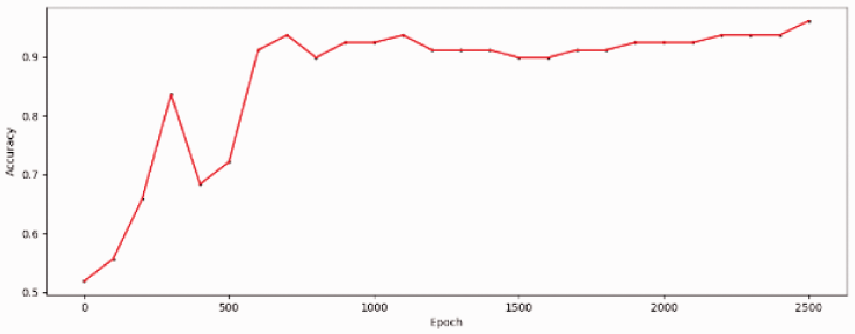
Accuracy of test set (LSTM).

When training the LSTM model, it can be seen from Figure 5 that there is an obvious rebound in the loss curve at 1900 times of training, because the loss of LSTM is flat to the change of parameters, some places are steep, when using gradient descent and encountering particularly steep places, it will jump out of local optimum, so the loss will suddenly increase, which is a normal phenomenon.

GRU model training

The data preprocessing of GRU model is the same as that of LSTM, and then the grid search method is used to determine several super parameter values in GRU model, such as the number of hidden layers and GRU layers. Through experiments, the number of hidden layers is 180, and the number of GRU layers is 2, which can make the performance of the model reach the best. Because of the same classification problem, the loss function and accuracy judgment of GRU model are the same as those of LSTM model.

Figure 7 shows the trend of loss with training times in the training set, and Figure 8 shows the trend of accuracy with training times in the test set. From the training results, it can be observed that the loss of the model decreases continuously with the increase of training times, and the accuracy of the test set increases continuously, which proves that the effect of the model is constantly becoming stronger. Finally, the loss decreased to 0.003 and the accuracy increased to 0.961.

Figure 7.

Loss of training set (GRU).

Figure 8.

Accuracy of test set (GRU).

GRU model training process also has the same problems as LSTM model training. Loss does not continue to decline with the number of training, but has ups and downs. The reason for this phenomenon is caused by local optimum, which is the same as LSTM.

Training comparison of different models with different data sets

In order to show the advantages of the LSTM and GRU models more clearly, this paper compares the performance of KNN, DT, and traditional neural network models. For more clearly, accuracy is an only index to measure the performance of the model, and these model data sets have passed five cross validation using the same data set for training and testing. Finally, each model is cycled 50 times, and the average and variance are used as the final score of each model.

KNN: As a traditional machine learning algorithm, k-Nearest Neighbor directly uses the scikit-learn deployment model. Firstly, the parameters of the KNN model, such as n-neighbor, weights and algorithm, are optimized by grid search, and the optimal setting of the model is determined.

DT: Decision Tree and KNN are both traditional machine learning algorithms, so scikit-learn is also used to deploy its training model, and grid search is used to optimize the parameters such as criterion, max_depth and splitter in the model, so as to achieve the optimal performance of the model.

Traditional neural network: back propagation neural network model is built by Tensor Flow framework, only one hidden layer is used to compare and deep learn differences. Firstly, the number of neurons in the hidden layer is searched, and the optimal setting is selected. After optimization, the network structure model of 36–500-4 is obtained. Relu is selected as the activation function, and the output layer is linear output with a learning rate of 0.01. Finally, to prevent over fitting, the dropout is set as 0.5.

After training and learning different data sets with different models, the results are as shown in Figures 9 to 14.

Figure 9.

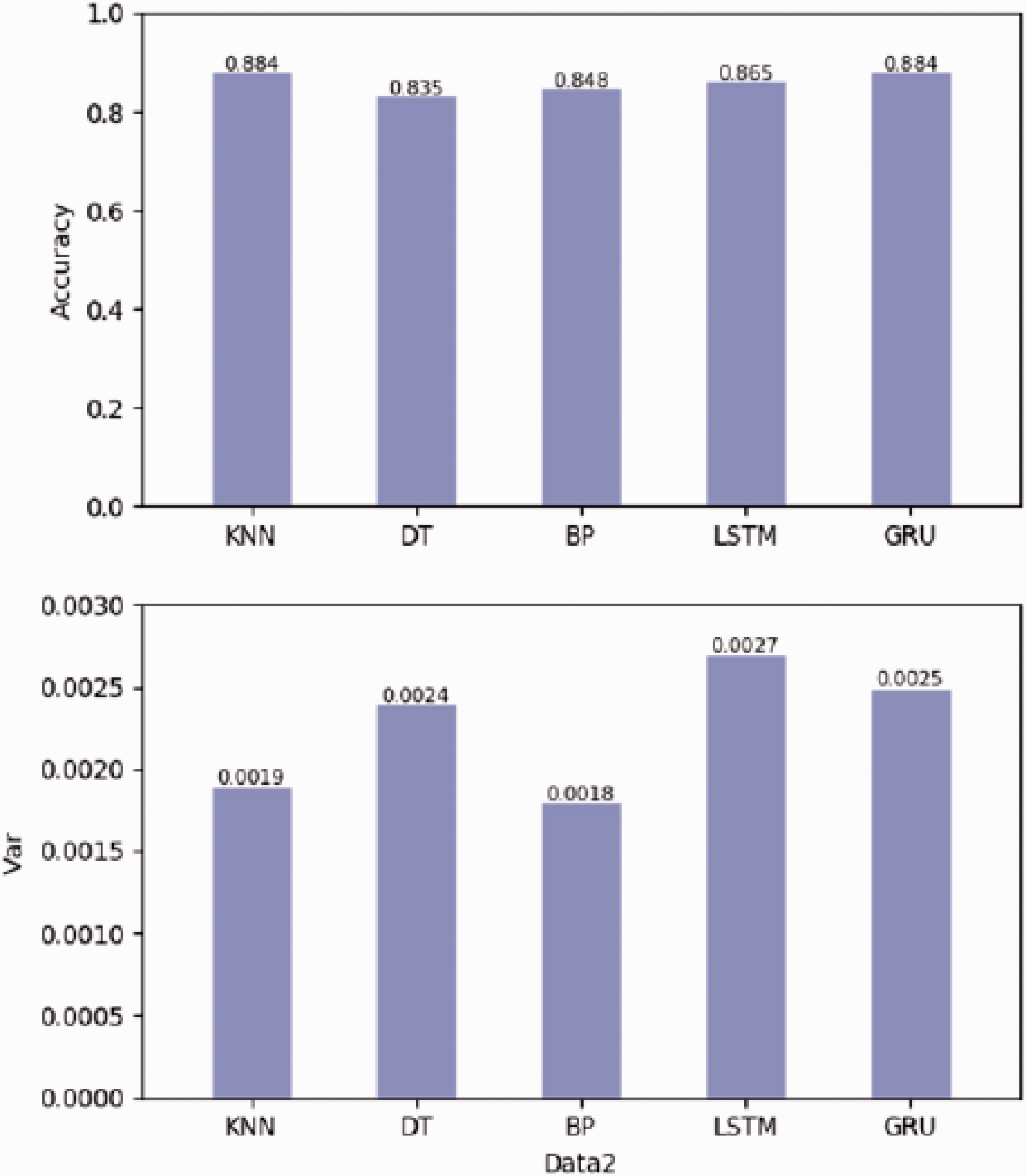
Data set 1 experimental results.

Figure 10.

Data set 2 experimental results.

Figure 11.

Data set 3 experimental results.

Figure 12.

Data set 4 experimental results.

Figure 13.

Data set 5 experimental results.

Figure 14.

Data set 6 experimental results.

Analysis of experimental results

First of all, according to the training results of each model in the original data set (data set 1), it can be seen that the accuracy of the traditional machine learning method and single hidden layer neural network prediction are lower than that of the LSTM and GRU models. Especially the BP model is far lower than that of LSTM and GRU, which cannot automatically extract features from the high-dimensional original data. Therefore, the prediction results are the worst, with only 41.2% accuracy. Although KNN and DT are lower than LSTM, they are also much higher than BP model. This means that traditional machine learning can automatically extract some features from the original data, but not the whole data set. The LSTM and GRU models use a multi hidden layer architecture, with a unique memory structure inside. They can selectively store the processing results of the previous time. When processing data at the current time point, they use the current input data and combine the previous impact factors stored by themselves to output the results. If the output of the current time is not associated with the previous data, they can also choose to forget the previously stored data. Only the current data input is used for processing and output to the next time point. Therefore, LSTM and GRU models can extract some features that traditional machine learning and BP models cannot. The results of variance show that the stability of each model is almost the same.

Additionally, according to the comparison of six data sets, it can be seen that LSTM and GRU are superior to the other three models in the processing of different data sets. And LSTM and GRU models can extract features that cannot be processed by other models. By comparing the structure of LSTM and GRU models with other models, it can be easily concluded that this is because of time feature. The variation of RNN can extract the time feature, and the forgetting gate and the reset gate can make the previous processing result as the input of the current time. LSTM and GRU models make their final prediction accuracy slightly higher than other models by processing time correlation. Therefore, data with time correlation, such as industrial big data, is more suitable to use LSTM and GRU models.

In addition to the influencing factors of time correlation, there are many abnormal data in the data set of job shop, and the structure of LSTM and GRU model can control whether the current input data can enter the current processing, so if there is abnormal data, LSTM and GRU model can also remove it and do not participate in the operation.

The performance of LSTM and GRU on different data sets is similar, but the internal storage unit structure of GRU is simpler than that of LSTM. Therefore, the speed of GRU is much faster than that of LSTM when training the model. And with the more layers of LSTM, the training time of GRU and LSTM will be more different. Through the experimental comparison, it can be concluded that GRU model takes far less time than LSTM model when the prediction effect is almost the same as LSTM model. Therefore, GRU model is better than LSTM model in processing industrial data.

To sum up, LSTM and GRU models have the advantages of big data processing of production process that traditional machine learning and BP neural network do not have, and GRU has more obvious advantages than LSTM through experiments.

Conclusion

As one of the most promising tools for deep learning, RNN has been applied to speech recognition, machine translation, text generation, emotion classification, video behavior recognition and other fields because of its unique cell structure which can store information, analyze and process complex content in information. In this paper, LSTM and GRU are applied to the processing of manufacturing big data. It is found that they have a natural advantage in processing the structure of manufacturing big data. Their unique storage structure can not only remove the noise in the data, but also extract the time characteristics of the data, and make more accurate prediction of the results. Compared with the traditional machine learning method and BP neural network, they have a significant improvement.

In the training process of LSTM and GRU models, there is often a loss value fluctuation, which causes the decrease of accuracy. Sometimes the final accuracy is not as high as the value in the training process, so the code can be improved, such as setting the loss threshold, selecting the model with higher accuracy value as the output result. With the research of RNN model, there are many revised RNN models. In the future work, a more suitable RNN model for processing manufacturing data should be found through improving LSTM and GRU.

Footnotes

Declaration of Conflicting Interests

The author(s) declared no potential conflicts of interest with respect to the research, authorship, and/or publication of this article.

Funding

The author(s) disclosed receipt of the following financial support for the research, authorship, and/or publication of this article: This work is financially supported by the China Postdoctoral Science Foundation under Grant 2018M643727, Natural Science Foundation of Shanxi Province under Grant 2019JM-099, National Natural Science Foundation of China under Grant 51975463.

ORCID iD

Chuang Wang

References

Hermann

Pentek

Otto

Design principles for industrie 4.0 scenarios. In: 2016 49th Hawaii international conference on system sciences (HICSS). Piscataway, NJ: IEEE, 2016, pp.3928–3937.

Da Xu

Internet of things in industries: a survey. IEEE Trans Ind Inf 2014; 10: 2233–2243.

Al-Fuqaha

Guizani

Mohammadi

, et al. Internet of things: a survey on enabling technologies, protocols, and applications. IEEE Commun Surv Tutorials 2015; 17: 2347–2376.

Want

An introduction to RFID technology. IEEE Pervasive Comput 2006; 5: 25–33.

Niu

Liu

Gao

, et al. Energy efficient task assignment with guaranteed probability satisfying timing constraints for embedded systems. IEEE Trans Parallel Distrib Syst 2014; 25: 2043–2052.

Akyildiz

Sankarasubramaniam

, et al. A survey on sensor networks. IEEE Commun Magaz 2002; 40: 102–114.

Zhong

Newman

Huang

, et al. Big data for supply chain management in the service and manufacturing sectors: challenges, opportunities, and future perspectives. Comput Ind Eng 2016; 101: 572–591.

Yin

Kaynak

Big data for modern industry: challenges and trends [point of view]. Proc Ieee 2015; 103: 143–146.

Rao

Babu

Shankar

, et al. Mining association rules based on Boolean algorithm – a study in large databases. IJMLC 2013; 3: 347–351.

10.

Barr

Bi-objective optimization based on compromise method for horizontal fragmentation in relational data warehouses. IJMLC 2013; 3: 250–254.

11.

Gierej

Big data in the industry-overview of selected issues. Manage Syst Prod Eng 2017; 25: 251–254.

12.

Satapathy

Maheshwari

Sai Hanuman

, et al. Integrated PSO and DE for data clustering. IJMLC 2012; 2: 839–843.

13.

Ritter

Advanced data processing in the business network system. IJMLC 2013; 3: 190–194.

14.

Hochreiter

Schmidhuber

Long short-term memory. Neural Comput 1997; 9: 1735–1780.

15.

Graves

Jaitly

Mohamed

Hybrid speech recognition with deep bidirectional LSTM. In: 2013 IEEE workshop on automatic speech recognition and understanding. Piscataway, NJ: IEEE, 2013, pp.273–278.

16.

Cho

Van Merriënboer

Gulcehre

, et al. Learning phrase representations using RNN encoder-decoder for statistical machine translation. arXiv Preprint arXiv:1406.1078, 2014;

17.

Mou

Ghamisi

Zhu

XX.

Deep recurrent neural networks for hyperspectral image classification.IEEE Trans Geosci Remote Sensing 2017; 55: 3639–3655.

18.

Tirkel

Forecasting flow time in semiconductor manufacturing using knowledge discovery in databases. Int J Prod Res 2013; 51: 5536–5548.

19.

Wang

Zhang

Big data analytics for forecasting cycle time in semiconductor wafer fabrication system. Int J Prod Res 2016; 54: 7231–7244.

20.

Chen

Wang

YC.

Incorporating the FCM–BPN approach with nonlinear programming for internal due date assignment in a wafer fabrication plant. Rob Comput-Integr Manuf 2010; 26: 83–91.

21.

Takeuchi

Ito

Fukumi

Novel approximate statistical algorithm for large complex datasets. IJMLC 2012; 2: 720–724.

22.

Deep learning based approach for bearing fault diagnosis. IEEE Trans Ind Applicat 2017; 53: 3057–3065.

23.

Fang

Guo

Liao

, et al. Big data driven jobs remaining time prediction in discrete manufacturing system: a deep learning-based approach. Int J Prod Res 2020; 58: 2751–2716.