An adaptive Cahn-Hilliard equation for enhanced edges in binary image inpainting

Abstract

We consider the Cahn-Hilliard equation for solving the binary image inpainting problem with emphasis on the recovery of low-order sets (edges, corners) and enhanced edges. The model consists in solving a modified Cahn-Hilliard equation by weighting the diffusion operator with a function which will be selected locally and adaptively. The diffusivity selection is dynamically adopted at the discrete level using the residual error indicator. We combine the adaptive approach with a standard mesh adaptation technique in order to well approximate and recover the singular set of the solution. We give some numerical examples and comparisons with the classical Cahn-Hillard equation for different scenarios. The numerical results illustrate the effectiveness of the proposed model.

Introduction

Image inpainting is a fundamental problem in image processing. It has interesting applications and has wide applications in different imaging fields, such as medical imaging, photoshop, augmented reality, robotic and even in daily life (see e.g., Bertalmio et al.^1,2; Chan and Shen ³ ; Esedoglu and Shen ⁴ ). It refers to restoring a damaged image with missing information. Various mathematical models have been proposed and discussed for this problem with different success rate. Among them, partial differential equations (PDEs) are widely used, and they showed good success mainly for cartoon and binary images Chan and Shen. ³ In this work, we are interested in the Cahn-Hilliard equation (CHE) and its application in binary images inpainting. The Cahn-Hilliard equation originally refers to the authors Cahn and Hilliard ⁵ and was introduced to phenomenologically describe the evolution of an interface between two state phases. It is a fourth-order semi-linear PDE which is derived from the $H^{-1}$ -gradient flow of the following Ginzburg-Landau energy

$$\frac{1}{2}{\displaystyle {\int }_{\Omega }|}\nabla u{|}^2+\frac{W(u)}{{\mathrm{ϵ}}^2}\text{d}x$$

(1)

where

$$W(u)=(1-u^2)u^2$$

is a smooth free energy Elliott, ⁶ called double-well potentials, which models the phase separation.

For binary image inpainting, Cahn-Hilliard equation was first exploited by Bertozzi et al.^7,8 by considering the following modified version

$$-\Delta (\Delta u-\frac{1}{{\mathrm{ϵ}}^2}W\prime (u))+\lambda (f-u)=0,\text{in}\Omega$$

(2)

Equation (2) is obtained by incorporating the fidelity part $\lambda (f-u)$ which keeps the image u close to the observed data f in the damaged domain $\Omega \mathrm{\setminus }D$ , where $D\subset \Omega$ is the user-supplied inpainting region and

$$\lambda (x)={\lambda }_0{\chi }_{\Omega \mathrm{\setminus }D}$$

where ${\chi }_{\Omega \mathrm{\setminus }D}$ is the indicator function of the subdomain $\Omega \mathrm{\setminus }D$ and ${\lambda }_0>0$ . The two state phases modelled by the Cahn-Hilliard equation can be seen as homogeneous regions in the image, while the interface between them plays the role of an edge. Because the double well potential W vanishes only at the values 0 and 1, the model (2) is appropriate for inpainting only two scale images.

A non-smooth version of Cahn-Hilliard equation was used in Bosch et al. ⁹ ; Blowey and Elliott^10,11 in image inpainting by considering the following non-smooth double obstacle potential

$$W(u)=\psi (u)+I_{[0,1]}(u)$$

(3)

where $\psi (u)=\frac{1}{2}u(1-u)$ and $I_{[0,1]}(u):=\{\begin{array}{l}\frac{1}{2}u(1-u),0\le u\le 1,\hfill \\ +\infty ,\text{Otherwise}.\hfill \end{array}$

This non-smooth double obstacle potential has the advantage of giving more intense colors and it then reveals the high contrast and the edges in the image. In this case, the full model consists in solving the following PDEs

$$-\Delta (\Delta u-\frac{1}{{\mathrm{ϵ}}^2}(\psi \prime (u)+\mu )+\lambda (f-u)=0,\text{in}\Omega$$

(4)

$$\mu \in \partial {\beta }_{[0,1]}(u)$$

(5)

$$0\le u\le 1\text{in}\Omega$$

(6)

$$\frac{\partial u}{\partial n}=\frac{\partial \Delta u}{\partial n}=0\text{on}\partial \Omega$$

(7)

where $\partial {\beta }_{[0,1]}(u)$ denotes the sub-differential of the non-smooth part

$${\beta }_{[0,1]}(u)={\displaystyle {\int }_{\Omega }{I}_{[0,1]}}\text{d}x$$

The system (4) to (7) leads to a variational inequality which requires the use of Lagrange multipliers associated with the constraints in equation (6). Those constraints can be also relaxed using Moreau-Yosida regularization, see Bosch et al. ⁹

The edge quality when using Cahn-Hilliard like models in image inpainting is related to the choice of the parameter ϵ, which usually affects the sharpness of the edges. A large value of ϵ is always needed in order to join edges over large distances, whereas, in the same time, small value is preferred to sharpen the edges as the contrast depends on the ϵ-jump. Thus, choosing ϵ to be constant, whether it is large or small, in the classical Cahn-Hilliard equation is not always relevant to inpaint large damaged areas due to the trade-off between inpainting of large areas and the sharpness of edges, see Bertozzi et al.^7,8; Bertozzi and Schönlieb. ¹² In practice, the authors in Bertozzi et al., ⁷ Bertozzi and Schönlieb ¹² used two step-process; they began the numerical computation with a large value of ϵ to reach a steady state. Then, they switch to a new system with a small value of ϵ using the previous result (i.e. computed with large ϵ) as initial data in order to sharpen the edges. This numerical adjustment of ϵ can be seen as an adaptive choice for ϵ, however, subjected to a hand tuning and being uniform in the entire domain.

In this work, we propose a model which can cope with the compromise between the inpainting of large areas and the sharpness of edges. We consider a weighted Cahn-Hilliard equation by adding a diffusion function α. More precisely, the model is given by the following equation

$$\{\begin{array}{l}{\partial }_{t}u-\Delta ({\Delta }_{\alpha }u-\frac{1}{{\mathrm{ϵ}}^2}W\prime (u))+\lambda (f-u)=0,\text{in}\Omega ,\hfill \\ {\Delta }_{\alpha }u-\frac{1}{{\mathrm{ϵ}}^2}W\prime (u)=0,\text{on}\partial \Omega ,\hfill \\ u=f,\text{on}\partial \Omega ,\hfill \end{array}$$

(8)

where ${\Delta }_{\alpha }:=\text{div }(\alpha (x)\nabla u)$ . The diffusion function α, which encodes different scales in the image, is dynamically chosen in order to control the amount of the smoothing of the operator. The benefits of the proposed approach have two folds:

1. The inpainting of large damaged domains by choosing the parameter ϵ sufficiently large.

2. The recovery of the fine features of the initial image by controlling the diffusion function α locally and adaptively depending on the position $x\in \Omega$ . This will help to achieve an inpainting process with high-contrasted and sharp edges.

In equation (8), we have chosen to use the smooth Cahn-Hilliard model, as it is more convenient for the numerical computation comparing to the non-smooth one. Equation (8) is obtained by considering the $H^{-1}$ gradient flow of the following Ginzburg-Landau type energy

$$E_1(u)={\displaystyle {\int }_{\Omega }\frac{\alpha (x)}{2}}|\nabla u{|}^2+\frac{W(u)}{{\mathrm{ϵ}}^2}\text{d}x$$

(9)

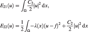
while the second fitting part can be derived from a gradient flow in L² for the following energy

$$E_2(u)=\frac{1}{2}{\displaystyle {\int }_{\Omega }\lambda }(x){(f-u)}^2\text{d}x$$

(10)

The aim is to simultaneously inpaint and sharpen the edges across large damaged domain. In fact, the parameter ϵ will deal with the inpainting a large damaged domain, while α will recover the singularities and sharp edges.

The article is organized as follows: In the next section, we show the well posedness of the stationary equation related to equation (8). Then, we construct a linearized version of equation (8) based on the convexity-splitting method. In the penultimate section is dedicated to the introduction of the adaptive strategy for the selection of the diffusion parameter α based on the residual error indicator. Finally, different numerical examples are outlined in Section 5 to show the efficiency and robustness of the proposed method.

H¹-weak solution of the stationary equation

We suppose that the domain Ω is partitioned into N disjoint sub-domains ${({\Omega }_{\ell })}_{\ell }$ such that α is given by the piecewise constant scalar function

$$\alpha ={\alpha }_{\ell },\text{in }{\Omega }_{\ell }$$

We denote ${\alpha }_m={\min }_{1\le \ell \le N}{\alpha }_{\ell }>0$ and ${\alpha }_M={\max }_{1\le \ell \le N}{\alpha }_{\ell }$ . For simplicity, we will use the homogeneous boundary condition of $u{|}_{\partial \Omega }=f{|}_{\partial \Omega }=0$ , and this condition is not a restrictive. Let $H^{-1}{(\Omega )}^{\hspace{0.17em}}$ be the dual space of $H_0^1(\Omega )$ ,

$${〈\phi ,\psi 〉}_{-1}:={\displaystyle {\int }_{\Omega }\nabla }{\Delta }^{-1}\phi \nabla {\Delta }^{-1}\psi \text{d}x$$

and induced by the following norm

$$\left|\right|\phi |{|}_{-1}:=\sqrt{{\displaystyle {\int }_{\Omega }{(\nabla {\Delta }^{-1}\phi )}^2}\text{d}x}$$

where the operator ${\Delta }^{-1}·$ is the inverse of the negative Laplacian with homogeneous Dirichlet boundary conditions. A weak solution of the stationary problem which corresponds to equation (8) is defined as a function u in the space $H_0^1(\Omega )$ such that

$${〈\alpha \nabla u,\nabla \varphi 〉}_2+{〈\frac{W\prime (u)}{{\mathrm{ϵ}}^2},\varphi 〉}_2-{〈\lambda (f-u),\varphi 〉}_{-1}=0,\forall \varphi \in H_0^1(\Omega )$$

(11)

and which, equivalently, solves the following system

$$\{\begin{array}{l}-{\Delta }_{\alpha }u+\frac{W\prime (u)}{{\mathrm{ϵ}}^2}+{\Delta }^{-1}({\lambda }_0(u-f))=0,\text{in}\Omega ,\hfill \\ {\Delta }_{\alpha }u+\frac{W\prime (u)}{{\mathrm{ϵ}}^2}=0,\text{on}\partial \Omega \hfill \end{array}$$

(12)

Proposition 1. For ${\lambda }_0\ge \frac{C}{{\mathrm{ϵ}}^4{\alpha }_{\mathit{min}}}$ , where C is a positive constant depending only on $\left|\Omega \right|,\left|D\right|$ , and W. For $f\in L^2(\Omega )$ , the weak problem (11) admits a solution $u\in H^1(\Omega )$ .

Proof. The proof can be done similarly to Bertozzi and Schönlieb ¹² ; Burger et al. ¹³ using classical calculus of variation analysis and fixed point techniques.

Theorem 2.1. Let $f\in L^2(\Omega )$ , the initial-boundary value problem (8) possesses a unique solution u which belongs to

$$C([0,T];L^2(\Omega ))\cap L^2(0,T;V),\mathrm{for every }T>0.$$

Proof. The proof is based on the results in Bertozzi et al. ⁷

Numerical algorithm

In this section, we present the numerical algorithm that we use to approximate the solution of the proposed modified Cahn-Hilliard evolution equation (8). More precisely, we use a semi-implicit approach called convexity splitting (CS) method (see Eyre ¹⁴ ) which was originally proposed by Yuille and Rangarajan ¹⁵ to solve general optimization problems. It was also applied for different nonlinear models such as the Cahn-Hilliard and Ohta-Kawasaki models (see Bertozzi and Schönlieb ¹² ; Kim and Shin ¹⁶ ). The idea of CS is to divide the energies (9) and (10) into two parts; a convex plus a concave one. The convex part is then treated implicitly, while the concave part is treated explicitly. We refer the reader to Elsey and Wirth ¹⁷ ; Hale ¹⁸ ; Shin et al. ¹⁹ for more details and various type of applications.

In our case, equation (8) can be written as

$${\partial }_{t}u=-\nabla E(u)$$

where $E(u)=E_1(u)-E_2(u)$ . Note that E₁ and E₂ are the functional given in equations (9) and (10), respectively. Then, we apply the convexity splitting scheme to the two parts $E_1(u)$ in equation (9) and $E_2(u)$ in equation (10) separately. More precisely, we write $E_1=E_{11}-E_{12}$ where

$$\begin{array}{l}{E}_{11}(u)=\frac{1}{2}{\displaystyle {\int }_{\Omega }\alpha }(x)|\nabla u{|}^2+\frac{C_1}{2}|u{|}^2\text{d}x,\\ E_{12}(u)={\displaystyle {\int }_{\Omega }-}\frac{1}{{\mathrm{ϵ}}^2}W(u)+\frac{C_1}{2}|u{|}^2\text{d}x\end{array}$$

It is clear that E₁₁ is strictly convex for any $C_1\ge 0$ , and the functional E₁₂ is strictly convex for all $\mathrm{ϵ}{C}_1>1$ . Similarly, assuming $E_2=E_{21}-E_{22}$ where

$$\begin{array}{l}{E}_{21}(u)={\displaystyle {\int }_{\Omega }\frac{C_2}{2}}|u{|}^2\text{d}x,\\ E_{22}(u)=\frac{1}{2}{\displaystyle {\int }_{\Omega }-}\lambda (x)(u-f{)}^2+\frac{C_2}{2}|u{|}^2\text{d}x\end{array}$$

E₂₂ is strictly convex if and only if $C_2>{\lambda }_0$ . Let $\Delta t$ be the discrete time step width, and write $t^n=n\Delta t$ , with $n=1,2,\dots ,T/\Delta t-1$ . In addition, let $u^n(x)$ be the approximate solution of the corresponding time-discrete numerical scheme of u(x, t) at time $t=t^n$ . Hence, the resulting time-stepping scheme for the splitting choices of the energies E₁ and E₂ is

$$\begin{array}{l}\frac{u^{n+1}-u^n}{\Delta t}=-{\nabla }_{H^{-1}}(E_{11}(u^{n+1})-E_{12}(u^n))\\ -{\nabla }_{L^2}(E_{21}(u^{n+1})-E_{22}(u^n))\end{array}$$

where ${\nabla }_{H^{-1}}$ and ${\nabla }_{L^2}$ are the descent gradients with respect to the $H^{-1}$ - and L²-inner product, respectively.

We obtain the following scheme

$$\begin{array}{l}\frac{u^{n+1}-u^n}{\Delta t}+\Delta {\Delta }_{\alpha }{u}^{n+1}-C_1\Delta u^{n+1}+C_2{u}^{n+1}\\ =\Delta \left(\frac{W\prime (u^n)}{{\mathrm{ϵ}}^2}\right)+\lambda (x)(u^n-f)-C_1\Delta u^n+C_2{u}^n\end{array}$$

(13)

Remark 1. In Bertozzi and Schönlieb, ¹² the authors proved that this time-stepping scheme is unconditionally stable in the sense that the numerical solution ${(u^n)}_{n\ge 0}$ is uniformly bounded on a finite time interval. The stability proof of this scheme in our case requires some modifications and the result still holds.

Space discretization

For space discretization, we will use mixed finite element method. We introduce the following auxiliary function

$$w^{n+1}=-{\Delta }_{\alpha }{u}^{n+1}+\frac{W\prime (u^n)}{{\mathrm{ϵ}}^2}$$

(14)

Then, from the PDEs (equation (13)), we get the following system

$$\{\begin{array}{l}\frac{u^{n+1}-u^n}{\Delta t}-\Delta w^{n+1}-C_1\Delta u^{n+1}+C_2{u}^{n+1}\hspace{0.17em}\hfill \\ =\lambda (x)(u^n-f)-C_1\Delta u^n+C_2{u}^n,\text{ in }\Omega ,\hfill \\ w^{n+1}=-{\Delta }_{\alpha }{u}^{n+1}+\frac{W\prime (u^n)}{{\mathrm{ϵ}}^2},\text{ in }\Omega ,\hfill \\ u^{n+1}=w^{n+1}=0,\text{ on }\partial \Omega \hfill \end{array}$$

(15)

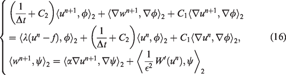
Multiplying the first and the second equations in equation (15) by two test functions $\varphi ,\psi \in H_0^1(\Omega )$ , respectively, then integrating over Ω, we obtain for all $\varphi \in H_0^1(\Omega )$ and $\psi \in H_0^1(\Omega )$ the following weak formulation

$$\{\begin{array}{l}(\frac{1}{\Delta t}+C_2){〈u^{n+1},\varphi 〉}_2+{〈\nabla w^{n+1},\nabla \varphi 〉}_2+C_1{〈\nabla u^{n+1},\nabla \varphi 〉}_2\hfill \\ ={〈\lambda (u^n-f),\varphi 〉}_2+(\frac{1}{\Delta t}+C_2){〈u^n,\varphi 〉}_2+C_1{〈\nabla u^n,\nabla \varphi 〉}_2,\hfill \\ {〈w^{n+1},\psi 〉}_2={〈\alpha \nabla u^{n+1},\nabla \psi 〉}_2+{〈\frac{1}{{\mathrm{ϵ}}^2}W\prime (u^n),\psi 〉}_2\hfill \end{array}$$

(16)

Proposition 2. For a fixed $u^n\in H_0^1(\Omega )$ , the system (16) has a unique solution $(u^{n+1},w^{n+1})\in H_0^1(\Omega )\times H_0^1(\Omega )$ .

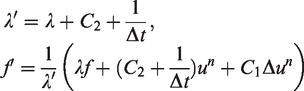
Proof. For a given $f\in L^2(\Omega ),u^n\in H_0^1(\Omega )$ , and let C₁, C₂, and $\Delta t$ are positive constants. We define

$$\begin{array}{l}\lambda \prime =\lambda +C_2+\frac{1}{\Delta t},\\ f\prime =\frac{1}{\lambda \prime }\left(\lambda f+(C_2+\frac{1}{\Delta t})u^n+C_1\Delta u^n\right)\end{array}$$

Then, with the above notations, the system (15) is equivalent to

$$\{\begin{array}{l}-{\Delta }_{\alpha }{u}^{n+1}-{\Delta }^{-1}(\lambda \prime (f\hspace{0.17em}\prime -u^{n+1}))=-\frac{W\prime (u^n)}{{\mathrm{ϵ}}^2},\text{ in }\Omega ,\hfill \\ {\Delta }_{\alpha }{u}^{n+1}+\frac{W\prime (u^n)}{{\mathrm{ϵ}}^2}=0,\text{ on }\partial \Omega \hfill \end{array}$$

(17)

Moreover, for fixed $u^n\in H_0^1(\Omega )$ , similarly to the system (12), we can prove equation (17) admits a unique solution $u^{n+1}$ . In addition, it is clear that the pair $(u^{n+1},w^{n+1}=-{\Delta }_{\alpha }{u}^{n+1}+\frac{W\prime (u^n)}{{\mathrm{ϵ}}^2})$ satisfies the system (16). To prove the uniqueness, let $(u_1^{n+1},w_1^{n+1})\in H_0^1(\Omega )\times H_0^1(\Omega )$ be another solution of the system (16). For all $(\varphi ,\psi )\in H_0^1(\Omega )\times H_0^1(\Omega )$ , we then have

$$\{\begin{array}{l}{〈\nabla (w^{n+1}-w_1^{n+1}),\nabla \varphi 〉}_2+{〈\lambda \prime (u^{n+1}-u_1^{n+1}),\varphi 〉}_2=0,\hfill \\ {〈\alpha \nabla (u^{n+1}-u_1^{n+1}),\nabla \psi 〉}_2-{〈w^{n+1}-w_1^{n+1},\psi 〉}_2=0\hfill \end{array}$$

(18)

Let ${({\zeta }_{\ell })}_{\ell =1}^I$ be a partition of unity associated to the decomposition ${({\Omega }_{\ell })}_{\ell =1}^I$ , and picking $\psi ={\alpha }_{\ell }^{-1}{\zeta }_{\ell }(w^{n+1}-w_1^{n+1})$ , in the second equation, we have the identity

$$\begin{array}{l}{\displaystyle {\int }_{{\Omega }_{\ell }}{\alpha }_{\ell }^{-1}}{\zeta }_{\ell }{(w^{n+1}-w_1^{n+1})}^2\text{d}x\\ ={\displaystyle {\int }_{{\Omega }_{\ell }}{\alpha }_{\ell }}\nabla (u^{n+1}-u_1^{n+1}){\alpha }_{\ell }^{-1}\nabla {\zeta }_{\ell }(w^{n+1}-w_1^{n+1})\text{d}x,\\ \forall \ell =1,\cdots ,I\end{array}$$

(19)

Integrating by parts twice the right-hand side and summing up, we obtain

$$\begin{array}{l}{\displaystyle \sum _{\ell =1}^I{\alpha }_{\ell }^{-1}}{\displaystyle {\int }_{{\Omega }_{\ell }}{\zeta }_{\ell }}{(w^{n+1}-w_1^{n+1})}^2\text{d}x\\ ={\displaystyle {\int }_{\Omega }{\alpha }_{\ell }}\nabla (u^{n+1}-u_1^{n+1})\nabla (w^{n+1}-w_1^{n+1})\text{d}x\ge 0\end{array}$$

(20)

By choosing the test function $\varphi =u^{n+1}-u_1^{n+1}$ in the first equation, using equation (20) and the positivity of C₁, C₂ and λ, we obtain

$$\begin{array}{l}{〈\lambda \prime (u^{n+1}-u_1^{n+1}),u^{n+1}-u_1^{n+1}〉}_2\\ =-{〈\nabla (u^{n+1}-u_1^{n+1}),\nabla (w^{n+1}-w_1^{n+1})〉}_2\le 0\end{array}$$

From the nonnegativity of $\lambda \prime$ , we get

$${〈\lambda \prime (u^{n+1}-u_1^{n+1}),u^{n+1}-u_1^{n+1}〉}_2=0$$

Therefore, $u^{n+1}=u_1^{n+1}$ , and consequently, $w^{n+1}=w_1^{n+1}$ .

Finite element discretization and adaptive strategy

In order to find the solution of this problem, we apply the finite element method. Let h > 0, Ω _h be a polygonal subset of Ω and ${\mathbb{T}}_h$ be a nondegenerate triangulation of the discrete domain Ω _h where each triangle or quadrilateral $K\in {\mathbb{T}}_h$ has maximum diameter bounded by h, satisfying the usual admissibility assumptions, i.e. the intersection of two different elements is either empty, a vertex, or a whole edge. We denote by $P_1(K)$ the space of all polynomials defined on triangular elements K. We introduce the following discrete space

$$X_h=\left\{v_h\in C(\overline{\Omega })|\forall K\in {\mathbb{T}}_h,v_h{|}_K\in P_1(K)\right\}\cap H_0^1(\Omega )$$

The finite discretization of equation (16) is defined by the following algebraic system

$$\begin{array}{l}(C_2+1/\Delta t)\mathbf{M}{u}^{n+1}+C_1\mathbf{K}{u}^{n+1}+\mathbf{K}{w}^{n+1}\\ =(C_2+1/\Delta t)\mathbf{M}{u}^n+C_1\mathbf{K}{u}^n+{\mathbf{M}}^{\lambda }{u}^n-\mathbf{F},\\ \mathbf{M}{w}^{n+1}-{\mathbf{K}}^{\alpha }{u}^{n+1}=\mathbf{R}\end{array}$$

where

$$\begin{array}{l}{\mathbf{M}}_{i,j}=(v_i,v_j),{\mathbf{M}}_{i,j}^{\lambda }=(\lambda v_i,v_j),\hspace{0.17em}\hfill \\ {\mathbf{K}}_{i,j}=(\nabla v_i,\nabla v_j),{\mathbf{K}}_{i,j}^{\alpha }=(\alpha \nabla v_i,\nabla v_j),\hspace{0.17em}\hfill \\ {\mathbf{F}}_i=(\lambda f,v_i),{\mathbf{R}}_i=(\frac{1}{{\mathrm{ϵ}}^2}W\prime (u^n),v_i)\hfill \end{array}$$

$(.,.)$ denotes the discrete L²-inner product, and ${\left\{v_i\right\}}_{i\in J}$ be a basis of X_h with J is the set of all vertices. We write the above system as follows

$$\left[\begin{array}{cc}{\mathbf{A}}_1& \mathbf{K}\\ -{\mathbf{K}}^{\alpha }& \mathbf{M}\end{array}\right]\left[\begin{array}{c}{u}^{n+1}\\ w^{n+1}\end{array}\right]=\left[\begin{array}{c}{\mathbf{b}}_1^n\\ {\mathbf{b}}_2^n\end{array}\right]$$

(21)

where ${\mathbf{A}}_1=(C_2+1/\Delta t)\mathbf{M}+C_1\mathbf{K},{\mathbf{b}}_1^n={\mathbf{A}}_1{u}^n+{\mathbf{M}}^{\lambda }{u}^n-\mathbf{F}$ and ${\mathbf{b}}_2^n=\mathbf{R}$ .

Adaptivity

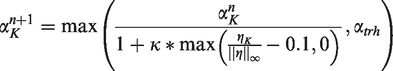
As mentioned in the introduction, the diffusion parameter α plays an important role in the inpainting process. Therefore, it is of interest to choose it based on a satiable strategy. Hence, we use an adaptive local procedure based on a residual error indicator. For each element K ∈  ${\mathbb{T}}_h$ , we use the following local discrete energy

$${\eta }_K={\alpha }_K^{\frac{1}{2}}\left|\right|\nabla u_h|{|}_{L^2(K)}$$

(22)

which contains information about the error distribution of the computed solution u_h and also acts as an edge detector. In fact, the discontinuities (edges) are contained in regions where the brightness changes abruptly and therefore where this error indicator is large. Thus, quantity is well suited to locally control and select the diffusion coefficient α using an adaptive strategy, see Belhachmi and Frédéric ²⁰ ; Theljani et al.^21,22 During the adaptation, we use the following formula for each triangle K

$${\alpha }_K^{n+1}=\max \left(\frac{{\alpha }_K^n}{1+\kappa *\max \left(\frac{{\eta }_K}{\left|\right|\eta |{|}_{\infty }}-0.1,0\right)},{\alpha }_{\mathit{trh}}\right)$$

where α_trh is a threshold parameter and κ is a coefficient chosen to control the rate of decreasing in α. In addition, we use a mesh-adaptation technique allowing a tight location of the singularities. It also permits both the refinement (near the edges) and the coarsening of the grid (in homogeneous area) in order to best fit the geometry of the image and to make the method considerably fast. The build mesh is done iteratively until a maximum number of iterations are reached. Our algorithm is described as follows.

Algorithm 1: Adaptive algorithm based image inpainting

1. Initialization: Start with the initial grid ${\mathbb{T}}_h^0$ and $\alpha (x)={\alpha }^0$ .

2. Iterations: For fixed function $\alpha (x)={\alpha }^k$ and mesh ${\mathbb{T}}_h^k$ , compute $u^{k+1}$ so using convexity splitting (CS) method.

 (a) Perform mesh adaptation to get the new mesh ${\mathbb{T}}_h^{K+1}$ with mesh refinement step (in our case using the metric adaptation with FreeFem++).

(b) Perform a local choice of $\alpha (x)$ to obtain new functions ${\alpha }_{k+1}$ .

3. Go to step (2) until convergence.

Remark 2. The advantages of this algorithm rely in two points: First, we make the “optimal” choice of the function α, following the map furnished by the error indicator ${({\eta }_K)}_{K\in T_h}$ , on each element K in order to approximate correctly the edges. Second, we build an adapted mesh ${\mathbb{T}}_h^1$ (in the sense of the finite element method, i.e. with respect to the parameter h) by cutting the elements K, close to the jump sets of u_h into a finite number of smaller elements to fit the edges, while, far from these jumps, the grid is coarsened.

Numeric

We present some numerical experiments to show the efficiency of our approach for image inpainting, and we compare it with classical Cahn-Hilliard equation Bertozzi et al. ⁷ In all examples, the damaged regions are marked with red and gray colors.

We use the Structural Similarity Index Measurement (SSIM) as an evaluation metric to compare both models and which is given by the following formula

$$\text{SSIM}=\frac{(2{\mu }_I{\mu }_{I_0}+c_1)(2{\sigma }_{I_1{I}_0}+c_2)}{({\mu }_I^2+{\mu }_{I_0}^2+c_1)({\sigma }_I^2+{\sigma }_{I_0}^2+c_2)}$$

where μ, ${\sigma }^2$ , σ are the mean, the variance, the covariance, respectively, and c₁ and c₂ are two positive parameters. The SSIM allows to estimate the quality of a reconstructed image with respect to its original version image. It takes a value between 0 and 1 where closer to 1 means a better inpainting process.

In Figure 1, we have chosen the same image presented by the authors Bertozzi et al. ⁷ The result using classical Cahn-Hilliard equation in Figure 1(b) was computed in a two steps process. In the first step, the authors solved their equation with a large value of ϵ, e.g. $\mathrm{ϵ}=0.1$ , until getting steady-state solution. In this step, the level lines are smoothly continued into the missing domain. In a second step, the previous result from step 1 was used as an initial time condition $u_{\alpha }^0$ for a smaller ϵ (e.g., $\mathrm{ϵ}=0.01$ ) in order to sharpen the contours. From the result of our model in Figure 1(c), we can see the corners are accurately approximated and the edges are properly and sharply inpainted contrary to the result of the classical Cahn-Hilliard model (Figure 1(b)). We also display in Figure 2 the evolution of the mesh at iteration 0, 3, 7 and 20, respectively. The first is the initial mesh ${\mathbb{T}}_h^0$ which is regular such that every node corresponds to a pixel in the image and the last one is the final coarsed mesh.

Figure 1.

Destroyed binary image and the solutions of the different models. (a) Damaged image, (b) model of Bertozzi et al., ⁷ SSIM = 0.89 and (c) New model, SSIM = 0.92.

Figure 2.

The adopted mesh refinement with iterations. (a) Iteration 0, (b) Iteration 3, (c) Iteration 7 and (d) Iteration 20.

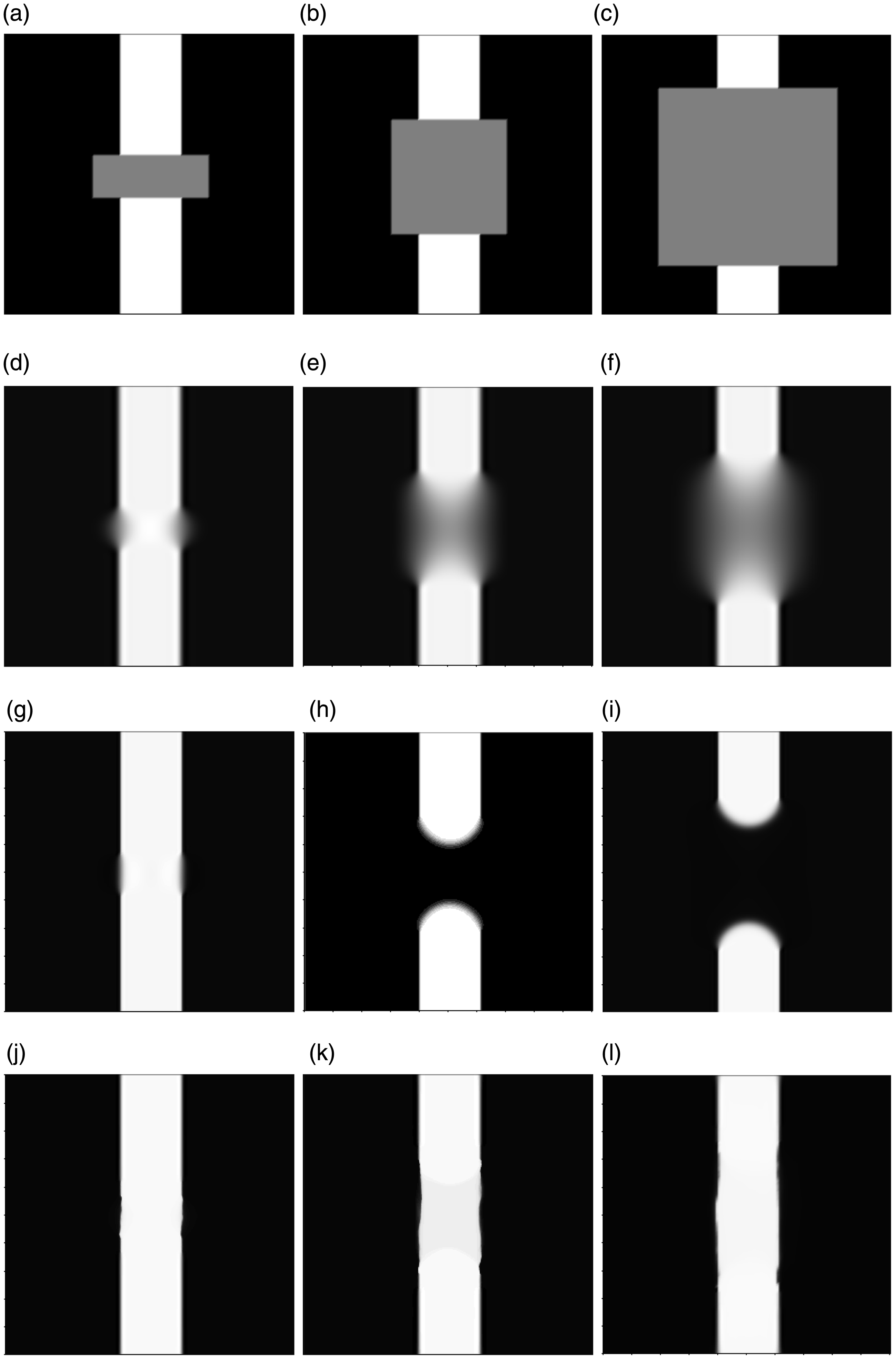
In the Figure 3, we compare both models in inpainting edges across large distance by considering three different inpainting scenarios (first line in Figure 3). The images in the second line were obtained using the classical Cahn-Hilliard model, where $\mathrm{ϵ}=0.8$ in all the domain Ω. The value $\mathrm{ϵ}=0.8$ is large enough and allows to join the both sides of the damaged stripe for the three scenarios. However, it leads to a very blurred edge because the contrast of the latter depends on the ϵ-jump. In another hand, if we choose a small value, i.e. $\mathrm{ϵ}=0.01$ (third line of Figure 3), the model is able to join the edges only for non-large damaged domain and fails to join them across large domains. Contrary, our proposed approach, see last line in Figure 3, gives successful result as the stripe is well inpainted and the edges are sharply recovered in all scenarios. We used $\mathrm{ϵ}=0.8$ in all the image domains Ω in order to match the edges and we adapted the diffusion function α to recover the singularities of the image, i.e. edges. Thus, we reconstruct edges across large domain and keeping them sharp enough. We tabulate the number of iterations and the SSIM values for the different models and the different scenarios in Table 1. It is clear that our model gives better results among in terms of SSIM and also necessitates less iterations.

Figure 3.

First line: Three different inpainting domains. Second line: Restored images by classical Cahn-Hilliard ( $\mathrm{ϵ}=0.8$ ). Third line: Restored images by classical Cahn-Hilliard ( $\mathrm{ϵ}=0.01$ ). Fourth one: Restored images by new model.

Table 1.

or comparison between the different models related to the example in Figure 3.

	Figure 3 (a)		Figure 3 (b)		Figure 3 (c)
	SSIM	#Iter.	SSIM	#Iter.	SSIM	#Iter.
Cahn-Hilliard with $\mathrm{ϵ}=0.8$	0.93	10	0.9	15	0.88	20
Cahn-Hilliard with $\mathrm{ϵ}=0.01$	0.97	20	0.85	26	0.83	26
New model	0.98	8	0.97	12	0.95	20

SSIM: Structural Similarity Index Measurement.

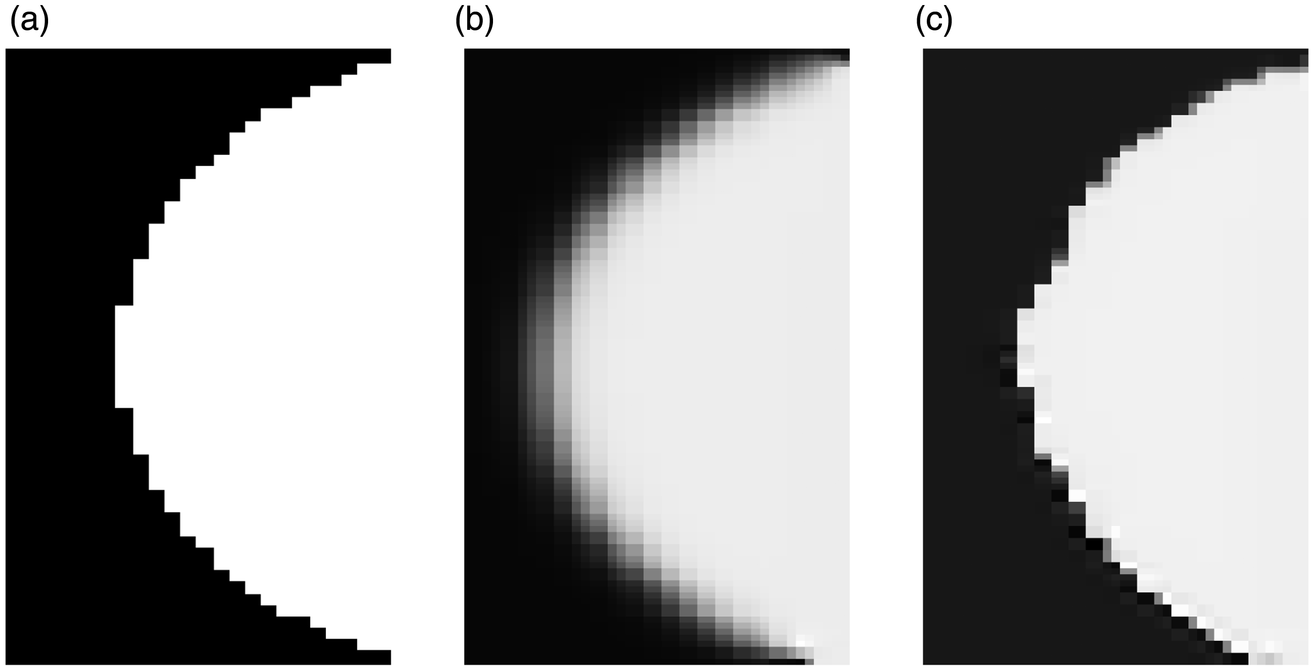
In Figure 4, we test our model in reconstructing damaged part of a disk in order to show the efficiency of the adaptive strategy for curvature reconstruction. Figure 4(a) is the initial damaged image f (inpainting region in red). In Figure 4(b), we display the inpainted images using the classical Cahn-Hilliard model for $\mathrm{ϵ}=0.01$ and after 16 time-iterations. The reconstructed edges clearly are blurred. In Figure 4(c), we show the result of our adaptive strategy using the error indicators η_K in equation (22). We initialized the algorithm with large value of α = 10 and we performed only 6 adaptive iterations to obtain. We also display zoomed regions in Figure 5 to highlight the main visual differences between the different results. The zoom captions prove that our model can effectively sharpen edges and preserve curvatures.

Figure 4.

From left to right: Damaged image, Cahn-Hiliard equation with constant $\alpha =0.01$ (SSIM = 0.96) and new model (SSIM = 0.98). (a) Damaged image, (b) Classical Cahn-Hiliard and (c) new model.

Figure 5.

Zoom captions from the test in Figure 4. (a) Referenced image, (b) Classical Cahn-Hiliard equation with α is fixed constant and (c) new model.

The last example in Figure 6 deals with real application for a binary QR-code image inpainting. It gives a promising result for corners and large gap reconstruction. The efficiency of our new approach can be seen in all the image domains, and in particular in the damaged region. In fact, all corners and edges were well reconstructed.

Figure 6.

From left to right and top to bottom: The referenced image, damaged image, restored image by the new model at iterations 4 and 33. (a) The referenced image, (b) damaged image, (c) new model at iteration 4, SSIM = 0.81 and (d) new model after 33 iterations, SSIM = 0.97.

Conclusion

In this paper, we have addressed a new approach for binary image inpainting problem based on a weighted Cahn-Hilliard equation. The weight parameter controls the over-smoothness of the operator and is chosen locally and adaptively based on the residual error indicator in each pixel of the image. In the numerical computation, we used the splitting convexity method in order to linearise the proposed non-linear equation. The experiment results show the good performance in recovering well enhanced edges in comparison with classical Cahn-Hilliard model.

References

1.
BertalmioMBertozziASapiroG. Navier-Stokes, fluid dynamics, and image and video inpainting. In: Proceedings of the international conference on computer vision and pattern recognition, Hauai, HI, 8-14 December, New York: IEEE, 2001, pp.355–362.
2.
BertalmioMSapiroGCasellesV, et al. Image inpainting. In: Proceedings of the 27th annual conference on computer graphics and interactive techniques. New York: ACM, 2000, pp.417–427.
3.
ChanTShenJ.Mathematical models for local non-texture inpainting. SIAM J Appl Math2002;
62: 1019–1043.
CahnJHilliardE.Free energy of a nonuniform system. I. Interfacial free energy. J Chem Phys1989;
28.
6.
ElliottCM. The Cahn-Hilliard model for the kinetics of phase separation. In: Mathematical models for phase change problems. Berlin: Springer, 1989, pp.35–73.
7.
BertozziAEsedogluSGilletteA.Analysis of a two-scale Cahn-Hilliard model for image inpainting. Multiscale Model Simul2007;
6: 913–936.
8.
BertozziAEsedogluSGilletteA.Inpainting of binary images using the Cahn-Hilliard equation. IEEE Trans Image Process2007;
16: 285–291.
9.
BoschJKayDStollM, et al.
Fast solvers for Cahn-Hilliard inpainting. SIAM J Imaging Sci2014;
7: 67–97.
10.
BloweyJFElliottCM.The Cahn-Hilliard gradient theory for phase separation with non-smooth free energy part I: mathematical analysis. Eur J Appl Math1991;
2: 233–280.
11.
BloweyJFElliottCM.The Cahn-Hilliard gradient theory for phase separation with non-smooth free energy part II: numerical analysis. Eur J Appl Math1992;
3: 147–179.
12.
BertozziASchönliebC-B.Unconditionally stable schemes for higher order inpainting. Commun Math Sci2011;
9: 413–457.
13.
BurgerMHeLSchönliebC-B.Cahn-Hilliard inpainting and a generalization for grayvalue images. SIAM J Imaging Sci2009;
2: 1129–1167.
14.
EyreDJ. An unconditionally stable one-step scheme for gradient systems. Unpublished article, 1998.
KimJShinJ.An unconditionally gradient stable numerical method for the Ohta-Kawasaki model. Bull Korean Math Soc2017;
54: 145–158.
17.
ElseyMWirthB.A simple and efficient scheme for phase field crystal simulation. Esaim: M2an2013;
47: 1413–1432.
18.
HaleJK.Asymptotic behavior of dissipative systems, no. 25 in mathematical surveys and monographs 025.
Providence, RI:
American Mathematical Society, 1988.
19.
ShinJLeeHGLeeJY.Unconditionally stable methods for gradient flow using convex splitting Runge–Kutta Scheme. J Comput Phys2017;
347: 367–381.
20.
BelhachmiZHechtF.Control of the effects of regularization on variational optic flow computations. J Math Imaging Vis2011;
40: 1–19.
21.
TheljaniABelhachmiZKallelMand Moakher M. A multiscale fourth-order model for the image inpainting and low-dimensional sets recovery. Math Meth Appl Sci2017;
40: 3637–3650.
22.
TheljaniABelhachmiZMoakherM.High-order anisotropic diffusion operators in spaces of variable exponents and application to image inpainting and restoration problems. Nonlinear Analysis: Real World Appl2019;