Sage Journals: Discover world-class research

Abstract

In this paper, we present firstly several one-step iterative methods including classical Newton’s method and Halley’s method for root-finding problem based on Thiele’s continued fraction. Secondly, by using approximants of the second derivative and the third derivative, we obtain an improved iterative method, which is not only two-step iterative method but also avoids calculating the higher derivatives of the function. Analysis of its convergence shows that the order of convergence of the modified iterative method is four for a simple root of the equation. Finally, to illustrate the efficiency and performance of the proposed method, we give some numerical experiments and comparison.

Keywords

Nonlinear equation Thiele’s continued fraction Viscovatov algorithm iterative method order of convergence

Introduction

In the last years, many higher order iterative methods have been developed to solve a root-finding problem. Iterative algorithm is an interesting and very ancient subject (see literature^1–19 and references therein), due to the importance of the topic in numerical analysis, engineering and applied problems such as economics analysis, physics, dynamical models, and so on.^20–23 In general, by using a variant of different techniques, such as Taylor series,^24–26 decomposition,^4,5,9 quadrature^2,12 and homotopy methods,^13,14 these iterative methods could be derived.

We consider a nonlinear equation f(x) = 0. Suppose that $f (x) \in C^{n} [a, b], n = 1, 2, 3, \dots$ and let $x^{*} \in [a, b]$ satisfy $f (x^{*}) = 0$ . It is well known that Newton’s method as below

x_{k + 1} = x_{k} - \frac{f (x_{k})}{f^{'} (x_{k})}

(1)

is a good choice for finding the approximate root of f(x) = 0, which is a one-step iterative method and has quadratic convergence for a simple zero of the nonlinear equation, as shown in the works.^24–26 If two steps of Newton iterative method are seen as one step, Traub considered the following iteration in Traub²⁴

{\begin{array}{l} y_{k} = x_{k} - \frac{f (x_{k})}{f^{'} (x_{k})}, \\ x_{k + 1} = y_{k} - \frac{f (y_{k})}{f' (y_{k})}, k = 0, 1, 2, \dots \end{array}

The two-step Newton’s method is fourth-order convergent. Apparently, this iterative method depends on the first derivatives at point x_k and another point y_k. This kind of dependence can spend more time to the application for the two-step Newton’s method. Moreover, the two-step method requires two function evaluations and two first derivative evaluations per iteration. Thus, both to reduce the total number of new function evaluations (that is, the values of f and its derivatives $f^{'}$ ) per iteration and to keep the order of convergence, constructing an efficient iterative method is the main motivation of this work.

In this paper, we start with using a continued fraction to establish several one-step iterative methods including classical Newton’s method and Halley’s method for solving nonlinear equations. In order to avoid calculating the high-order derivatives of the function, then we employ the approximants of the higher derivatives to improve the presented iterative method. As a result, we construct an iterative formula without calculating the high-order derivatives. Unlike the above two-step Newton’s method, the proposed method only requires to calculate the values of the function f twice and the derivative $f^{'}$ at x_k once for each iteration step. It is clear that the advantage of the proposed method can save mathematical labor by eliminating one derivative evaluation at y_k. Furthermore, we prove that the order of convergence of the modified iterative method is four for a simple root of the equation. At last, we give some numerical experiments and comparison to illustrate the efficiency and performance of the proposed method.

The rest of this paper is organized as follows. In the next section we present some preliminaries for Thiele’s continued fraction and of iterative methods. In the subsequent section, we propose firstly several one-step iterative scheme based on the expansion of Thiele’s continued fraction. Then, we improve the presented iterative method to obtain an iterative formula without calculating the high-order derivatives, and we prove that the modified method is fourth-order convergent at least. In the penultimate section, we give numerical examples to show the performance of the presented method and compare it with other high-order methods. Finally, we draw conclusions from the experiment results of numerical examples in the last section.

Preliminaries

In this section, we briefly recall some basic definitions and results for Thiele’s continued fraction and the relative speed of convergence of iterative schemes. Some surveys and complete literatures on continued fractions and the speed of convergence of iterative methods could be found in Tan et al.,^27,28 Traub,²⁴ Gautschi²⁵ and Burden et al.²⁶ For simplicity throughout this paper we let $ℝ$ stand for a real numbers set.

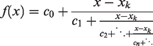
Definition 2.1 Assume ${c_{i} | c_{i} \in ℝ, i = 0, 1, 2, \dots}$ and ${x_{j} | x_{j} \in ℝ, j = 0, 1, 2, \dots}$ are two sets of real numbers. The continued fraction as below

c_{0} + \frac{x - x_{0}}{c_{1} + \frac{x - x_{1}}{c_{2} + ⋱ + \frac{x - x_{n - 1}}{c_{n} + ⋱}}}

(2)

is called Thiele’s continued fraction.

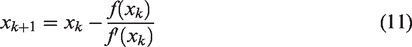
Definition 2.2 For equation (2) in Definition 2.1, the following continued fraction

c_{0} + \frac{x - x_{0}}{c_{1} + \frac{x - x_{1}}{c_{2} + ⋱ + \frac{x - x_{n - 1}}{c_{n}}}}

(3)

is defined as the n-th truncated Thiele’s continued fraction.

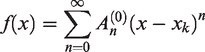
Let $A_{i}^{(0)}$ denote the coefficients of Taylor polynomial as

A_{i}^{(0)} = \frac{f^{(i)} (x_{k})}{i!}, i = 0, 1, 2, \dots

For the relation between the coefficients $A_{i}^{(0)}, i = 0, 1, 2, \dots$ , of Taylor’s expansion and the coefficients $c_{i} \in ℝ, i = 0, 1, 2, \dots$ , of Thiele’s continued fraction, we provide straightforward a lemma as follows without trying to prove it.

Lemma 2.1 (Viscovatov algorithm) Suppose that the function f(x) is n times differentiable on an interval $[a, b]$ . If f(x) can be expanded into the following Thiele’s continued fraction about the point $x_{k} \in [a, b]$

f (x) = c_{0} + \frac{x - x_{k}}{c_{1} + \frac{x - x_{k}}{c_{2} + ⋱ + \frac{x - x_{k}}{c_{n} + ⋱}}}

and Taylor series about the point x_k

f (x) = \sum_{n = 0}^{\infty} A_{n}^{(0)} {(x - x_{k})}^{n}

where

A_{n}^{(0)} = \frac{f^{(n)} (x_{k})}{n!}, n = 0, 1, 2, \dots

. Then the coefficients

c_{n}, n = 0, 1, 2, \dots

, can be calculated by using Viscovatov algorithm as follows^27,28

{\begin{array}{l} c_{0} = A_{0}^{(0)}, \\ c_{1} = 1 / A_{1}^{(0)}, \\ A_{i}^{(1)} = - A_{i + 1}^{(0)} / A_{1}^{(0)}, i \geq 1, \\ c_{l} = A_{1}^{(l - 2)} / A_{1}^{(l - 1)}, l \geq 2, \\ A_{i}^{(l)} = A_{i + 1}^{(l - 2)} - c_{l} A_{i + 1}^{(l - 1)}, i \geq 1, l \geq 2 \end{array}

On the other hand, we look back upon the relative speed of convergence of the iterative scheme. Firstly, we need to give a procedure for measuring how rapidly a sequence converges. Secondly, we require a definition for determining the speed of an iterative scheme.

Definition 2.3 Assume a sequence ${x_{k}}_{k = 0}^{\infty}$ converges to ξ, with $x_{k} \neq ξ$ for all $k, k = 0, 1, 2, \dots$ . If there exist two positive constants γ and τ such that

\lim_{k \to \infty} \frac{| x_{k} - ξ |}{| x_{k - 1} - ξ |^{τ}} = γ

(4)

then

{x_{k}}_{k = 0}^{\infty}

converges to ξ of order τ, and γ is called asymptotic error constant.

Definition 2.4 Assume a sequence ${x_{k}}_{k = 0}^{\infty}$ is generated by using an iterative technique of the form $x_{k} = φ (x_{k - 1})$ , for an initial approximation x₀ and each $k \geq 1$ . If the sequence ${x_{k}}_{k = 0}^{\infty}$ converges to the solution $ξ = φ (ξ)$ of order τ, then the order of convergence of the iterative scheme $x_{k} = φ (x_{k - 1})$ is said to be τ.

The iterative methods

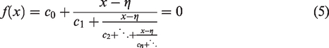
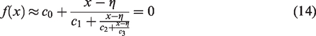
Now, we consider iterative methods to find a simple root of a nonlinear equation f(x) = 0. Let p be a simple root of the equation f(x) = 0 and suppose that η is an initial guess sufficiently close to p. Using Thiele’s continued fraction, we have

f (x) = c_{0} + \frac{x - η}{c_{1} + \frac{x - η}{c_{2} + ⋱ + \frac{x - η}{c_{n} + ⋱}}} = 0

(5)

where η is the initial approximation for a zero. It follows from Viscovatov algorithm (Lemma 2.1) that

c_{0} = f (η)

(6)

c_{1} = \frac{1}{f^{'} (η)}

(7)

c_{2} = - \frac{2 {f^{'}}^{2} (η)}{f^{″} (η)}

(8)

and

c_{3} = \frac{3 {f^{″}}^{2} (η)}{2 {f^{'}}^{2} (η) f^{‴} (η) - 3 f^{'} (η) {f^{″}}^{2} (η)}

(9)

Considering the first truncated Thiele’s continued fraction for equation (5), we have

c_{0} + \frac{x - η}{c_{1}} = 0

Solving for $x - η$ yields

x - η = - c_{0} c_{1}

(10)

From equation (10), we can have easily

x = η - c_{0} c_{1}

This sets the stage for the following Newton’s method. Letting $η = x_{k}$ and $x = x_{k + 1}$ , then we get

Algorithm 3.1 Starting with an initial approximation x₀ and considering equations (6) and (7), we can obtain the iterative sequence ${x_{k}}_{k = 0}^{\infty}$ by

x_{k + 1} = x_{k} - \frac{f (x_{k})}{f^{'} (x_{k})}

(11)

for all k > 0.

Algorithm 3.1 is the well-known Newton’s method for root-finding of nonlinear equation. The order of its convergence is quadratic.^24–26

Also, taking into account the second truncated Thiele’s continued fraction for equation (5), one can have

c_{0} + \frac{x - η}{c_{1} + \frac{x - η}{c_{2}}} = 0

Solving for x gives

x = η - \frac{c_{0} c_{1} c_{2}}{c_{0} + c_{2}}

(12)

which sets the stage for the following method. Letting

η = x_{k}

and

x = x_{k + 1}

, then we have

Algorithm 3.2 Starting with an initial approximation x₀ and considering equations (6) to (8), one can get the iterative sequence ${x_{k}}_{k = 0}^{\infty}$ by

x_{k + 1} = x_{k} - \frac{2 f (x_{k}) f^{'} (x_{k})}{2 {f^{'}}^{2} (x_{k}) - f (x_{k}) f^{″} (x_{k})}

(13)

for all k > 0.

Algorithm 3.2 is known as Halley’s method for solving nonlinear equation, which has cubic convergence.^25,26

Again, by using the third truncated Thiele’s continued fraction for f(x) expanded about x_k, one has the following approximation formula

f (x) \approx c_{0} + \frac{x - η}{c_{1} + \frac{x - η}{c_{2} + \frac{x - η}{c_{3}}}} = 0

(14)

Substituting equation (10) into equation (14) gives

c_{0} + \frac{x - η}{c_{1} + \frac{x - η}{c_{2} + \frac{- c_{0} c_{1}}{c_{3}}}} = 0

(15)

Solving equation (15) for x yields

x = η - \frac{{(c_{0} c_{1})}^{2} - c_{0} c_{1} c_{2} c_{3}}{c_{0} c_{1} - (c_{0} + c_{2}) c_{3}}

(16)

Let us set equation (16) as the stage for a new method, and use $η = x_{k}$ and $x = x_{k + 1}$ in equation (16). Then we obtain the following iterative method.

Algorithm 3.3 Starting with an initial approximation x₀ and replacing equation (16) with equations (6) to (9), the iterative sequence ${x_{k}}_{k = 0}^{\infty}$ is generated by the following iterative scheme

x_{k + 1} = x_{k} - \frac{f (x_{k}) \begin{array}{l} (6 f^{' 2} (x_{k}) f^{″} (x_{k}) - 3 f (x_{k}) {f^{″}}^{2} (x_{k}) \\ + 2 f (x_{k}) f^{'} (x_{k}) f^{‴} (x_{k})) \end{array}}{{2 f' (x_{k}) \begin{array}{l} (3 f^{' 2} (x_{k}) f^{″} (x_{k}) - 3 f (x_{k}) {f^{″}}^{2} (x_{k}) \\ + f (x_{k}) f^{'} (x_{k}) f^{‴} (x_{k})) \end{array}}}

(17)

for all $k ⩾ 1$ .

Algorithm 3.3 is a one-step method, which could be used for solving nonlinear equation. Obviously, in order to implement this iterative method, we have to calculate the second derivative and the third derivative of the function f(x), which may cause inconvenience. For the sake of overcoming the drawback, we introduce approximants of the second derivative and the third derivative by means of Taylor series, which is a very important idea and plays a significant part in developing some iterative methods without calculating the higher derivatives. To be more precise, letting $y_{k} = x_{k} - f (x_{k}) / f' (x_{k})$ , and then expanding $f (y_{k})$ into third Taylor series about the point x_k yields

\begin{array}{l} f (y_{k}) \approx f (x_{k}) + f' (x_{k}) (y_{k} - x_{k}) \\ + \frac{1}{2!} f ″ (x_{k}) {(y_{k} - x_{k})}^{2} + \frac{1}{3!} f^{'''} (x_{k}) {(y_{k} - x_{k})}^{3} \end{array}

which means

f^{‴} (x_{k}) \approx \frac{3 f^{2} (x_{k}) f' (x_{k}) f ″ (x_{k}) - 6 f (y_{k}) f^{' 3} (x_{k})}{f^{3} (x_{k})}

(18)

Substituting equation (18) into equation (17), one can get the following iterative method.

Algorithm 3.4 Starting with an initial approximation x₀, the iterative sequence ${x_{k}}_{k = 0}^{\infty}$ is generated by the following iterative scheme

x_{k + 1} = x_{k} - \frac{{\begin{matrix} 4 f (x_{k}) f (y_{k}) {f^{'}}^{4} (x_{k}) - 4 f^{3} (x_{k}) f^{' 2} (x_{k}) f^{″} (x_{k}) \\ + f^{4} (x_{k}) {f^{″}}^{2} (x_{k}) \end{matrix}}}{{\begin{matrix} 4 f (y_{k}) f^{' 5} (x_{k}) + 2 f^{2} (x_{k}) f^{″} (x_{k}) \\ (f (x_{k}) f^{″} (x_{k}) - 2 f^{' 2} (x_{k})) \end{matrix}}}

(19)

where

y_{k} = x_{k} - \frac{f (x_{k})}{f' (x_{k})}

for all

k ⩾ 1

It is obvious to see that the iterative method equation (19) needs to calculate the second derivative of the function f(x). In order to avoid computing the second derivative, we introduce an approximant of the second derivative by using Taylor series. Similarly, expanding $f (y_{k})$ into second Taylor series about the point x_k yields

\begin{matrix} f (y_{k}) \approx f (x_{k}) + (y_{k} - x_{k}) f^{'} (x_{k}) + \frac{1}{2!} {(y_{k} - x_{k})}^{2} f^{″} (x_{k}) \end{matrix}

which implies

f^{″} (x_{k}) \approx \frac{2 f (y_{k}) {f^{'}}^{2} (x_{k})}{f^{2} (x_{k})}

(20)

Using equation (20) in equation (19), one can get the following iterative method free from second derivatives.

Algorithm 3.5 Starting with an initial approximation x₀, the iterative sequence ${x_{k}}_{k = 0}^{\infty}$ is generated by the following iterative scheme

y_{k} = x_{k} - \frac{f (x_{k})}{f^{'} (x_{k})}

(21)

x_{k + 1} = x_{k} - \frac{(f (x_{k}) - f (y_{k})) f (x_{k})}{(f (x_{k}) - 2 f (y_{k})) f^{'} (x_{k})}

(22)

for all $k ⩾ 1$ .

Algorithm 3.4 and Algorithm 3.5 are two-step iterative methods. Especially for Algorithm 3.5, it does not require to compute the high-order derivatives. But more importantly, the characteristic of Algorithm 3.5 is that per iteration it requires two evaluations of the function and one of its first derivative. The efficiency of this method is better than that of the well-known other methods involving the second-order derivative of the function.

Convergence analysis

In this section we take into account the convergence criteria of Algorithm 3.5.

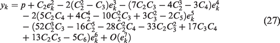
Theorem 4.1 Let $p \in [a, b]$ be a solution of the equation f(x) = 0. Suppose, in addition, that f(x) is sufficiently differentiable function in a neighborhood of the point p. If the initial approximation x₀ is sufficiently near to p, then the order of convergence of the two-step iterative scheme defined by Algorithm 3.5 is four.

Proof. By assumption, p is a solution of the equation f(x) = 0, so f(p) = 0. Let e_k be the error at k-th iteration, then one has $e_{k} = x_{k} - p$ . Consider the Taylor polynomial for $f (x_{k})$ expanded about p, one can have

\begin{array}{l} f (x_{k}) = f^{'} (p) e_{k} + \frac{1}{2!} f^{″} (p) e_{k}^{2} + \frac{1}{3!} f^{‴} (p) e_{k}^{3} + \frac{1}{4!} f^{(4)} (p) e_{k}^{4} \\ + \frac{1}{5!} f^{(5)} (p) e_{k}^{5} + \frac{1}{6!} f^{(6)} (p) e_{k}^{6} + O (e_{k}^{7}) \end{array}

(23)

f (x_{k}) = f' (p) (C_{1} e_{k} + C_{2} e_{k}^{2} + C_{3} e_{k}^{3} + C_{4} e_{k}^{4} + C_{5} e_{k}^{5} + C_{6} e_{k}^{6} + O (e_{k}^{7}))

(24)

f^{'} (x_{k}) = f^{'} (p) (C_{1} + 2 C_{2} e_{k} + 3 C_{3} e_{k}^{2} + 4 C_{4} e_{k}^{3} + 5 C_{5} e_{k}^{4} + 6 C_{6} e_{k}^{5} + O (e_{k}^{6}))

(25)

where $C_{i} = \frac{1}{i!} \frac{f^{(i)} (p)}{f^{'} (p)}, i = 1, 2, \dots$ . It is clear that $C_{1} = 1$ . From equations (24) and (25), one has

\begin{array}{l} \frac{f (x_{k})}{f^{'} (x_{k})} = e_{k} - C_{2} e_{k}^{2} + 2 (C_{2}^{2} - C_{3}) e_{k}^{3} + (7 C_{2} C_{3} - 4 C_{2}^{3} - 3 C_{4}) e_{k}^{4} \\ + 2 (5 C_{2} C_{4} + 4 C_{2}^{4} - 10 C_{2}^{2} C_{3} + 3 C_{3}^{2} - 2 C_{5}) e_{k}^{5} \\ + (52 C_{2}^{3} C_{3} - 16 C_{2}^{5} - 28 C_{2}^{2} C_{4} - 33 C_{2} C_{3}^{2} \\ + 17 C_{3} C_{4} + 13 C_{2} C_{5} - 5 C_{6}) e_{k}^{6} + O (e_{k}^{7}) \end{array}

(26)

Substituting equation (26) into equation (21) in Algorithm 3.5, one can get

\begin{array}{l} y_{k} = p + C_{2} e_{k}^{2} - 2 (C_{2}^{2} - C_{3}) e_{k}^{3} - (7 C_{2} C_{3} - 4 C_{2}^{3} - 3 C_{4}) e_{k}^{4} \\ - 2 (5 C_{2} C_{4} + 4 C_{2}^{4} - 10 C_{2}^{2} C_{3} + 3 C_{3}^{2} - 2 C_{5}) e_{k}^{5} \\ - (52 C_{2}^{3} C_{3} - 16 C_{2}^{5} - 28 C_{2}^{2} C_{4} - 33 C_{2} C_{3}^{2} + 17 C_{3} C_{4} \\ + 13 C_{2} C_{5} - 5 C_{6}) e_{k}^{6} + O (e_{k}^{7}) \end{array}

(27)

Using Taylors series for $f (y_{k})$ expanded about p, we have

\begin{array}{l} f (y_{k}) = f' (p) [C_{2} e_{k}^{2} - 2 (C_{2}^{2} - C_{3}) e_{k}^{3} - (7 C_{2} C_{3} - 5 C_{2}^{3} - 3 C_{4}) e_{k}^{4} \\ - 2 (5 C_{2} C_{4} + 6 C_{2}^{4} - 12 C_{2}^{2} C_{3} + 3 C_{3}^{2} - 2 C_{5}) e_{k}^{5} \\ + (28 C_{2}^{5} - 73 C_{2}^{3} C_{3} + 34 C_{2}^{2} C_{4} + 37 C_{2} C_{3}^{2} \\ - 17 C_{3} C_{4} - 13 C_{2} C_{5} + 5 C_{6}) e_{k}^{6} + O (e_{k}^{7})] \end{array}

(28)

Therefore, combining equations (24) and (28), one can have

\begin{array}{l} (f (x_{k}) - f (y_{k})) f (x_{k}) \\ = f^{' 2} (p) [e_{k}^{2} + C_{2} e_{k}^{3} + 2 C_{2}^{2} e_{k}^{4} - (3 C_{2}^{3} - 6 C_{2} C_{3} - C_{4}) e_{k}^{5} \\ + (7 C_{2}^{4} - 15 C_{2}^{2} C_{3} + 5 C_{3}^{2} + 8 C_{2} C_{4} - 2 C_{5}) e_{k}^{6} \\ + (44 C_{2}^{3} C_{3} - 16 C_{2}^{5} - 24 C_{2} C_{3}^{2} - 22 C_{2}^{2} C_{4} \\ + 14 C_{3} C_{4} + 10 C_{2} C_{5} - 3 C_{6}) e_{k}^{7} + O (e_{k}^{8})] \end{array}

(29)

Also, from equations (24), (28) and (25), one has

\begin{array}{l} (f (x_{k}) - 2 f (y_{k})) f^{'} (x_{k}) \\ = {f^{'}}^{2} (p) [e_{k} + C_{2} e_{k}^{2} + 2 C_{2}^{2} e_{k}^{3} - (2 C_{2}^{3} - 5 C_{2} C_{3} + C_{4}) e_{k}^{4} \\ + (4 C_{2}^{4} - 8 C_{2}^{2} C_{3} + 3 C_{3}^{2} + 6 C_{2} C_{4} - 2 C_{5}) e_{k}^{5} \\ - (8 C_{2}^{5} - 20 C_{2}^{3} C_{3} + 8 C_{2} C_{3}^{2} + 12 C_{2}^{2} C_{4} \\ - 7 C_{3} C_{4} - 7 C_{2} C_{5} + 3 C_{6}) e_{k}^{6} \\ - 4 (28 C_{2}^{6} - 91 C_{2}^{4} C_{3} - 9 C_{3}^{3} + 44 C_{2}^{3} C_{4} \\ + 5 C_{4}^{2} + 73 C_{2}^{2} C_{3}^{2} - 18 C_{2}^{2} C_{5} \\ + 9 C_{3} C_{5} + 6 C_{2} C_{6} - 46 C_{2} C_{3} C_{4}) e_{k}^{7} + O (e_{k}^{8})] \end{array}

(30)

Dividing equation (29) by equation (30) gives

\begin{array}{l} \frac{(f (x_{k}) - f (y_{k})) f (x_{k})}{(f (x_{k}) - 2 f (y_{k})) f' (x_{k})} \\ = e_{k} + (C_{2} C_{3} - C_{2}^{3}) e_{k}^{4} \\ + 2 (2 C_{2}^{4} + C_{3}^{2} + C_{2} C_{4} - 4 C_{2}^{2} C_{3}) e_{k}^{5} + O (e_{k}^{6}) \end{array}

(31)

So, from equation (22) in Algorithm 3.5, equation (31) and $e_{k + 1} = x_{k + 1} - p$ , one can obtain

\begin{array}{l} x_{k + 1} = p + (C_{2}^{3} - C_{2} C_{3}) e_{k}^{4} \\ - 2 (2 C_{2}^{4} + C_{3}^{2} + C_{2} C_{4} - 4 C_{2}^{2} C_{3}) e_{k}^{5} + O (e_{k}^{6}) \end{array}

(32)

that is

e_{k + 1} = (C_{2}^{3} - C_{2} C_{3}) e_{k}^{4} + O (e_{k}^{5})

(33)

which shows that the order of convergence of Algorithm 3.5 is four according to Definition 2.3 and Definition 2.4. We have shown Theorem 4.1.□

Numerical examples

In order to verify the performance of the fourth-order method defined by Algorithm 3.5 (abbreviated as Alg.3.5), we present some numerical results on some test equations. Also, we compare their results with Newton’s method (NM for short), Halley’s method (HM for short) and the modified Householder method (MHM for short) with fourth-order convergence that suggested by Noor and Gupta.¹¹ Starting with an given initial approximation x₀, all numerical computations are carried out by using Mathematica software. For $ε = 10^{- 14}$ , we choose the following stopping criteria so that the computer programs for iterative computations are terminated when the criteria are satisfied simultaneously:

$| x_{k + 1} - x_{k} | < ε$

$| f (x_{k + 1}) | < ε$

The test equations are presented as below, most of them could be found in the literatures^17–19 or some references mentioned previously.

\begin{array}{l} f_{1} (x) = x^{2} - e^{x} - 3 x + 2 = 0, f_{2} (x) = x^{3} + 4 x^{2} - 25 = 0, \\ f_{3} (x) = \cos x - x = 0, f_{4} (x) = x^{3} - 10 = 0, \\ f_{5} (x) = x^{2} - x e^{x} + \cos x = 0, f_{6} (x) = x^{2} + \sin \frac{x}{5} - \frac{1}{4} = 0, \\ f_{7} (x) = e^{x^{2} + 7 x - 30} - 1 = 0, f_{8} (x) = \sin^{2} x - x^{2} + 1 = 0 \end{array}

Displayed in Table 1 are the different test equations $f_{i} = 0, i = 1, 2, \dots, 8$ , the initial approximation x₀, the number of iterations k to approximate the solution, the approximate solution x_k, the values $| x_{k} - x_{k - 1} |$ and $| f (x_{k}) |$ . From Table 1, it is clear that Algorithm 3.5 is compatible with the method such as NM, HM and MHM.

Table 1.

Numerical experiments and comparison for different iterative methods.

Method	Equation	x ₀	k	x_k	$\| x_{k} - x_{k - 1} \|$	$\| f (x_{k}) \|$
NM	$f_{1} = 0$	3.6	8	0.25753028543986076045536730493724178138	$6.52 \times 10^{- 29}$	$3.50 \times 10^{- 46}$
HM	$f_{1} = 0$	3.6	6	0.25753028543986076045536730493724178138	$4.79 \times 10^{- 37}$	$1.57 \times 10^{- 46}$
MHM	$f_{1} = 0$	3.6	5	0.25753028543986076045536730493724178138	$1.89 \times 10^{- 22}$	$1.18 \times 10^{- 45}$
Alg.3.5	$f_{1} = 0$	3.6	4	0.25753028543986076045536730493724178138	$2.54 \times 10^{- 19}$	$4.87 \times 10^{- 44}$
NM	$f_{2} = 0$	3.5	7	2.03526848118195915354755041547361249916	$6.36 \times 10^{- 28}$	$2.90 \times 10^{- 47}$
HM	$f_{2} = 0$	3.5	6	2.03526848118195915354755041547361249916	$1.97 \times 10^{- 39}$	$5.77 \times 10^{- 47}$
MHM	$f_{2} = 0$	3.5	5	2.03526848118195915354755041547361249916	$8.23 \times 10^{- 36}$	$1.28 \times 10^{- 45}$
Alg.3.5	$f_{2} = 0$	3.5	4	2.03526848118195915354755041547361249916	$3.44 \times 10^{- 30}$	$3.08 \times 10^{- 45}$
NM	$f_{3} = 0$	1	5	0.73908513321516064165531208767387340401	$6.39 \times 10^{- 21}$	$1.51 \times 10^{- 41}$
HM	$f_{3} = 0$	1	4	0.73908513321516064165531208767387340401	$3.37 \times 10^{- 29}$	$5.06 \times 10^{- 49}$
MHM	$f_{3} = 0$	1	4	0.73908513321516064165531208767387340401	$1.18 \times 10^{- 35}$	$3.31 \times 10^{- 48}$
Alg.3.5	$f_{3} = 0$	1	3	0.73908513321516064165531208767387340401	$1.09 \times 10^{- 18}$	$7.46 \times 10^{- 47}$
NM	$f_{4} = 0$	–1	7	2.15443469003188372175929356651935049526	$1.70 \times 10^{- 22}$	$1.87 \times 10^{- 43}$
HM	$f_{4} = 0$	–1	7	2.15443469003188372175929356651935049526	$6.00 \times 10^{- 19}$	$4.59 \times 10^{- 44}$
MHM	$f_{4} = 0$	–1	5	2.15443469003188372175929356651935049526	$1.14 \times 10^{- 34}$	$2.71 \times 10^{- 47}$
Alg.3.5	$f_{4} = 0$	–1	5	2.15443469003188372175929356651935049526	$1.02 \times 10^{- 33}$	$9.66 \times 10^{- 43}$
NM	$f_{5} = 0$	2	8	0.63915409633200758106478062050024025359	$5.71 \times 10^{- 21}$	$6.21 \times 10^{- 41}$
HM	$f_{5} = 0$	2	5	0.63915409633200758106478062050024025359	$5.81 \times 10^{- 22}$	$6.94 \times 10^{- 46}$
MHM	$f_{5} = 0$	2	5	0.63915409633200758106478062050024025359	$3.75 \times 10^{- 19}$	$2.73 \times 10^{- 44}$
Alg.3.5	$f_{5} = 0$	2	4	0.63915409633200758106478062050024025359	$2.17 \times 10^{- 15}$	$1.00 \times 10^{- 43}$
NM	$f_{6} = 0$	1	7	0.40999201798913713162125837649907538612	$1.19 \times 10^{- 28}$	$7.55 \times 10^{- 48}$
HM	$f_{6} = 0$	1	5	0.40999201798913713162125837649907538612	$4.79 \times 10^{- 36}$	$8.13 \times 10^{- 50}$
MHM	$f_{6} = 0$	1	5	0.40999201798913713162125837649907538612	$5.25 \times 10^{- 38}$	$6.28 \times 10^{- 47}$
Alg.3.5	$f_{6} = 0$	1	4	0.40999201798913713162125837649907538612	$1.23 \times 10^{- 28}$	$7.91 \times 10^{- 46}$
NM	$f_{7} = 0$	3.5	13	3.00000000000000000000000000000000000000	$4.21 \times 10^{- 25}$	$3.63 \times 10^{- 44}$
HM	$f_{7} = 0$	3.5	7	3.00000000000000000000000000000000000000	$5.19 \times 10^{- 16}$	$1.08 \times 10^{- 44}$
MHM	$f_{7} = 0$	3.5	6	3.00000000000000000000000000000000000000	$1.36 \times 10^{- 24}$	$8.83 \times 10^{- 43}$
Alg.3.5	$f_{7} = 0$	3.5	6	3.00000000000000000000000000000000000000	$6.93 \times 10^{- 17}$	$8.48 \times 10^{- 41}$
NM	$f_{8} = 0$	–1	7	–1.40449164821534122603508681778686807718	$7.33 \times 10^{- 26}$	$6.00 \times 10^{- 47}$
HM	$f_{8} = 0$	–1	5	–1.40449164821534122603508681778686807718	$1.02 \times 10^{- 38}$	$2.40 \times 10^{- 48}$
MHM	$f_{8} = 0$	–1	5	–1.40449164821534122603508681778686807718	$8.22 \times 10^{- 34}$	$3.94 \times 10^{- 46}$
Alg.3.5	$f_{8} = 0$	–1	4	–1.40449164821534122603508681778686807718	$5.64 \times 10^{- 28}$	$8.12 \times 10^{- 45}$

Clearly, $x^{*} = 3$ is an exact solution of the equation $f_{7} = 0$ . Let ${x_{n}, n = 1, 2, \dots, k, \dots}$ denote the sequence generated by any iterative method. Shown in Table 2 are the different iterative methods, the test equation $f_{7} = 0$ , the initial approximation x₀, the cumulative count n, the approximate solution x_n of each iteration, the values $| x_{n} - 3 |$ and $| f (x_{n}) |$ . Table 2 mainly illustrates the relative speed of convergence of the sequences to 3 when the initial approximation $x_{0} = 3.5$ . It is easy to see that the fourth-order convergent sequence that generated by Alg.3.5 is within $10^{- 41}$ of 3 by the sixth term. At least 13 terms are needed to ensure this accuracy for the quadratically convergent sequence which generated by Newton iterative method. Just as Theorem 4.1 shows that fourth-order convergent sequences generally converge much more quickly than those that have low order convergence.

Table 2.

The relative speed of convergence of the sequences by different iterative methods.

Method	Equation	x ₀	n	${x_{n}}$	$\| x_{n} - 3 \|$	$\| f (x_{n}) \|$
NM	$f_{7} = 0$	3.5	1	3.42865506283005651245721073000655709096	$4.29 \times 10^{- 1}$	$3.15 \times 10^{2}$
			2	3.35671923435846878717900312491876046905	$3.57 \times 10^{- 1}$	$1.16 \times 10^{2}$
			3	3.28441981122350293301087227610438508013	$2.84 \times 10^{- 1}$	$4.27 \times 10^{1}$
			4	3.21240630845112338607950153061433380389	$2.12 \times 10^{- 1}$	$1.56 \times 10^{1}$
			5	3.14241815947802526994541960762590326219	$1.42 \times 10^{- 1}$	$5.50 \times 10^{0}$
			6	3.07872591444877280795742106579227547418	$7.87 \times 10^{- 2}$	$1.80 \times 10^{0}$
			7	3.02986671328086231576490110603292132687	$2.99 \times 10^{- 2}$	$4.76 \times 10^{- 1}$
			8	3.00518216043983687455684490043015144276	$5.18 \times 10^{- 3}$	$6.97 \times 10^{- 2}$
			9	3.00017276403899187393669369452989768051	$1.73 \times 10^{- 4}$	$2.25 \times 10^{- 3}$
			10	3.00000019615891595773288643949423192716	$1.96 \times 10^{- 7}$	$2.55 \times 10^{- 6}$
			11	3.00000000000025306874011878291631803157	$2.53 \times 10^{- 13}$	$3.29 \times 10^{- 12}$
			12	3.00000000000000000000000042121106213522	$4.21 \times 10^{- 25}$	$5.48 \times 10^{- 24}$
			13	3.00000000000000000000000000000000000000	$4.77 \times 10^{- 45}$	$3.63 \times 10^{- 44}$
HM	$f_{7} = 0$	3.5	1	3.35601116577588568424558312154122759624	$3.56 \times 10^{- 1}$	$1.15 \times 10^{2}$
			2	3.21112901168050819815797000684949896354	$2.11 \times 10^{- 1}$	$1.53 \times 10^{1}$
			3	3.07807397692207490178726191469322843597	$7.81 \times 10^{- 2}$	$1.78 \times 10^{0}$
			4	3.00617947727528652556626267615414160179	$6.18 \times 10^{- 3}$	$8.37 \times 10^{- 2}$
			5	3.00000332721627045019400114474122902304	$3.33 \times 10^{- 6}$	$4.33 \times 10^{- 5}$
			6	3.00000000000000051895693141726273814255	$5.19 \times 10^{- 16}$	$6.75 \times 10^{- 15}$
			7	3.00000000000000000000000000000000000000	$2.22 \times 10^{- 45}$	$1.08 \times 10^{- 44}$
MHM	$f_{7} = 0$	3.5	1	3.22147926950672397692904786913974804090	$2.21 \times 10^{- 1}$	$1.77 \times 10^{1}$
			2	2.97890333863655565021657260124804199973	$2.11 \times 10^{- 2}$	$2.40 \times 10^{- 1}$
			3	3.00041785542541819593006067606805136507	$4.18 \times 10^{- 4}$	$5.45 \times 10^{- 3}$
			4	2.99999999684674501872507771319677283455	$3.15 \times 10^{- 9}$	$4.10 \times 10^{- 8}$
			5	3.00000000000000000000000135619706129043	$1.36 \times 10^{- 24}$	$1.76 \times 10^{- 23}$
			6	3.00000000000000000000000000000000000000	$9.97 \times 10^{- 44}$	$8.83 \times 10^{- 43}$
Alg.3.5	$f_{7} = 0$	3.5	1	3.32770201961387298232542827485346691464	$3.28 \times 10^{- 1}$	$7.78 \times 10^{1}$
			2	3.15616031883867475772422389675496118063	$1.56 \times 10^{- 1}$	$6.80 \times 10^{0}$
			3	3.02435629509809135524330861400534569356	$2.44 \times 10^{- 2}$	$3.73 \times 10^{- 1}$
			4	3.00002940997206443891702473123340661668	$2.94 \times 10^{- 5}$	$3.82 \times 10^{- 4}$
			5	3.00000000000000006931645429656286350195	$6.93 \times 10^{- 17}$	$9.01 \times 10^{- 16}$
			6	3.00000000000000000000000000000000000000	$9.62 \times 10^{- 42}$	$8.48 \times 10^{- 41}$

Conclusion

From the section, it is evident that we have obtained several iterative methods including classical Newton’s method and Halley’s method based on the approximation formula of Thieles continued fraction. In order to avoid calculating the higher derivatives of the function, we have improved the proposed iterative method by using approximants of the second derivative and the third derivative. So we have gotten a modified iterative method free from the higher derivatives of the function. We have proved that the order of convergence of the method suggested by Algorithm 3.5 is four. Numerical experiments and comparison have shown in Tables 1 and 2 that the iterative scheme in Algorithm 3.5 is more efficient and performs better than classical Newton’s method, Halley’s method and the modified Householder method introduced by Noor and Gupta.¹¹

Footnotes

Declaration of Conflicting Interests

The author(s) declared no potential conflicts of interest with respect to the research, authorship, and/or publication of this article.

Funding

The author(s) disclosed receipt of the following financial support for the research, authorship, and/or publication of this article: This work was supported partially by the Natural Science Key Foundation of Education Department of Anhui Province (grant no. KJ2013A183), the Project of Leading Talent Introduction and Cultivation in Colleges and Universities of Education Department of Anhui Province (grant no. gxfxZD2016270) and the Incubation Project of the National Scientific Research Foundation of Bengbu University (grant no. 2018GJPY04).

References

Amat

Busquier

Gutierrez

JM.

Geometric construction of iterative functions to solve nonlinear equations. J Comput Appl Math 2003; 157: 197–205.

Frontini

Sormani

Third-order methods from quadrature formulae for solving systems of nonlinear equations. Appl Math Comput 2004; 149: 771–782.

Chun

A geometric construction of iterative functions of order three to solve nonlinear equations. Comput Math Appl 2007; 53: 972–976.

Abbasbandy

Improving Newton-Raphson method for nonlinear equations by modified Adomian decomposition method. Appl Math Comput 2003; 145: 887–893.

Chun

Iterative methods improving Newtons method by the decomposition method. Comput Math Appl 2005; 50: 1559–1568.

Kou

Wang

A composite fourth-order iterative method for solving non-linear equations. Appl Math Comput 2007; 184: 471–475.

Wang

Kou

A new modified secant-like method for solving nonlinear equations. Comput Math Appl 2010; 60: 1633–1638.

Noor

Shah

FA.

A family of iterative schemes for finding zeros of nonlinear equations having unknown multiplicity. Appl Math Inf Sci 2014; 8: 2367–2373.

Shah

Noor

MA.

Some numerical methods for solving nonlinear equations by using decomposition technique. Appl Math Comput 2015; 251: 378–386.

10.

Kwun

Saqib

Fahad

, et al. A new cubically convergent iterative method for solving nonlinear equations. Int J Pure Appl Math 2016; 111: 67–76.

11.

Noor

Gupta

Modified Householder iterative method free from second derivatives for nonlinear equations. Appl Math Comput 2007; 190: 1701–1706.

12.

Cordero

Torregrosa

JR.

Variants of Newton’s method using fifth-order quadrature formulas. Appl Math Comput 2007; 190: 686–698.

13.

Golbabai

Javidi

A new family of iterative methods for solving system of nonlinear algebraic equations. Appl Math Comput 2007; 190: 1717–1722.

14.

Noor

MA.

Iterative methods for nonlinear equations using homotopy perturbation technique. Appl Math Inform Sci 2010; 4: 227–235.

15.

Morlando

A class of two-step Newton’s methods with accelerated third-order convergence. Gen Math Notes 2015; 29: 17–26.

16.

Thukral

New modification of Newton method with third-order convergence for solving nonlinear equations of type

f (0) = 0

. Am J Comput Appl Math 2016; 6: 14–18.

17.

Saqib

Iqbal

Some multi-step iterative methods for solving nonlinear equations. Open J Math Sci 2017; 1: 25–33.

18.

Qureshi

UK.

A new accelerated third-order two-step iterative method for solving nonlinear equations. Math Theory and Modeling 2018; 8: 64–68.

19.

Ali

Aslam

Ali

, et al. New family of iterative methods for solving nonlinear models. Discrete Dyn Nat Soc 2018; 2018: 1–12.

20.

Cichocki

Unbehauen

Neural networks for optimization and signal processing. New York: John Wiley & Sons, 1993.

21.

Sciavicco

Siciliano

Modelling and control of robot manipulators. London: Springer-Verlag, 2000.

22.

Miljković

Miladinović

Stanimirović

, et al. Application of the pseudoinverse computation in reconstruction of blurred images. Filomat 2012; 26: 453–465.

23.

Roland

Beim

PG.

Inverse problems in neural field theory. SIAM J Appl Dynam Sys 2009; 8: 1405–1433.

24.

Traub

JF.

Iterative methods for the solution of equations. New York: Prentice-Hall, 1964.

25.

Gautschi

Numerical analysis. 2nd ed. Boston: Birkhauser, 2012.

26.

Burden

Faires

Burden

RL.

Numerical analysis. 10th ed. Boston: Cengage Learning, 2015.

27.

Tan

JQ.

The theory of continued fraction and its applications. Beijing: Science Press, 2007.

28.

Tan

JQ.

The limiting case of Thiele’s interpolating continued fraction expansion. J Comput Math 2001; 19: 433–444.

Fourth-order iterative method without calculating the higher derivatives for nonlinear equation

Abstract

Keywords

Introduction

Preliminaries

The iterative methods

Convergence analysis

Numerical examples

Conclusion

Footnotes

Declaration of Conflicting Interests

Funding

References