Image segmentation by improved minimum spanning tree with fractional differential and Canny detector

Abstract

In this study, we propose an algorithm that uses an improved Minimum Spanning Tree algorithm and a modified Canny edge detector to segment images that contain a considerable amount of noises. First, we use our modified Canny operator to pre-process an image, and record the obtained object boundary information; then, we apply the improved Minimum Spanning Tree algorithm to associate the above information with boundary points in order to separate edges into two classes in the image, namely the inner and boundary regions. In particular, Minimum Spanning Tree algorithm is improved by using Fractional differential and combining the functions of the intra-regional and inter-regional differences with a function for edge weights. Based on the experimental results, compared with the other four exiting algorithms, the new algorithm has the higher accuracy and the better effect for noised image segmentation.

Introduction

Image segmentation is a process that involves extracting targets or regions of interest from images. In particular, in the image segmentation process, the characteristics of gray scale, texture, color, and other characteristics in the image can be utilized to divide the image into several regions that have internal homogeneity. Since 1971, when Zahn first applied the graph theory for image segmentation and data clustering, ¹ the study for graph-based image segmentation has become a hot topic for research worldwide; considering this, the various graph-based image segmentation algorithms have been developed with different advantages based on sound mathematical concepts. It should be noted that, in graph-based image segmentation algorithms, the boundary of a region is the same as the edge of the region. Therefore, the extracted boundary will always be closed, even without using additional conditions or criteria.

In 1993, the graph cuts segmentation criterion was introduced by Wu and Leahy. ² It involves cutting the edge that has the smallest similarity between pixels; however, this method is prone to producing small image regions. Hence, Shi and Malik studied a normalized cut algorithm that considers the global information of an image to maximize the differences between the regions as well as similarities within the regions based on Wu and Leahy’s graph cuts segmentation criterion, thus overcoming the above-mentioned disadvantages. ³ Boykov and Funka-Lea explored an optimization framework for the energy function using graph cuts based on the properties of an area in a manner similar to the Mumford-Shah functional. ⁴ In addition, they applied their framework for N-dimensional image segmentation to obtain the global optimum, and found it to be efficient and robust for practical applications. Sharon et al. ⁵ described a top-down hierarchical image segmentation algorithm based on graph theory, calculated the coupling edge weight to obtain the subdivision graph, selected several seeds to roughly segment the image iteratively, and obtained the saliency map and extracted significant targets from the image. Their algorithm is not only efficient, but also leads to the accurate segmentation results. Furthermore, Wieclawak and Pietka modified the Live Wire algorithm by integrating the Wavelet transform with the fuzzy C means clustering method to obtain a cost function, and used graph theory for the segmentation of medical computed tomography (CT) and magnetic resonance (MR) images. ⁶ Gopalakrishnan et al. suggested a method to extract significant targets in images through random walks of the image graph. ⁷ In particular, first, they obtained the global attributes of an image based on the detected seed nodes by using the Markov random walk, and then they computed the local properties using the sparse k-regular graph to determine the background and foreground seed nodes via stepwise semi-supervised learning. Their results were good in terms of target extraction. Egger et al. developed a scale fixed template-based paradigm for complex images, ⁸ in which the gray level of the target area is the similar to that of the background, they introduced the concept of “template shape” to sample non-uniform and non-equidistant nodes in graph. Then, they applied their paradigm for the processing of two-dimensional and three-dimensional brain tumor images. Chen et al. presented a k clustering and graph-cuts-based image segmentation algorithm, ⁹ which enabled automatic image segmentation of cardiac dual-source CT images and accurately estimated the structure of the heart. In 2004, Felzenszwalb and Huttenlocher proposed a “small region merging” image segmentation criterion, ¹⁰ which entails that, when the internal differences in an area are greater than the differences between different areas, then the two homogeneous regions are identified and merged together so that the graph-based algorithm can extract the characteristics of an image in a faster manner. Considering this advantage, our study is based on this algorithm. It should be noted that, in the past few years, several other studies related to this research topic have been conducted in references.^11–14

The above-mentioned algorithms were studied only for specific, special engineering images; however, none of the existing image segmentation algorithms can be standard. Based on our experiments, for the images in this study, the effect of these previously algorithms is not ideal. In particular, the drawbacks of these previous graph-based algorithms are that the larger the parameters are set to, the more the details of the image are lost, whereas small parameters might lead to over-segmentation, in addition, because the image segmentation scale cannot be correctly determined in the previous algorithms, the foreground and background of an image are incorrectly partitioned. To overcome some of these problems and enable optimal edge detection algorithm available, the Canny operator was proposed by Canny in 1986. ¹⁵ In general, it is a multilevel edge detection operator. The optimal edge detection includes the following: (1) good detection: identifying the actual edges in an image as accurately as possible by minimizing the error rate; (2) good location: detecting edges as close to the actual edges as possible; and (3) minimal response: marking edges only once a single edge exists, and noise should not be identified as an edge. Thus, it is possible to use Fractional differential to enhance week edges^16,17 and combine the Canny operator with a graph-based image segmentation algorithm to overcome over-merging when the parameters are set as relatively large.

This remainder of this paper is organized as follows: the Modified Canny operator section describes the modified Canny operator as well as its differences compared with the traditional operator. Then, the improved minimum spanning tree (MST), its relevance, fractional differential, and its comparison with the other similar algorithms are presented in the Modified minimum spanning tree algorithm and Canny operator section 3. Finally, the Conclusions section provides our conclusions.

Modified Canny operator

Because the Canny operator only uses a single scale to not only suppress noise, but also detect edges, it has two problems: a small scale is sensitive to noise, and a large scale leads to loss in edge information. Furthermore, even if a so-called appropriate scale is found out, it will still require a compromise between the sensitivity and accuracy of the detection results compared with those that could be obtained using the large or small scales. To address this issue, Bao et al. ¹⁸ enhanced the Canny edge detector using scale multiplication in order to strengthen the edges in an image while effectively suppressing noise. In this manner, on pre-sorting the pixels, the edges can be divided into two classes while constructing a graph G; in particular, one class is associated with the edge points wherein at least one of the two nodes is connected the edges to be an edge point, whereas the other class includes nodes that are not associated with any edges.

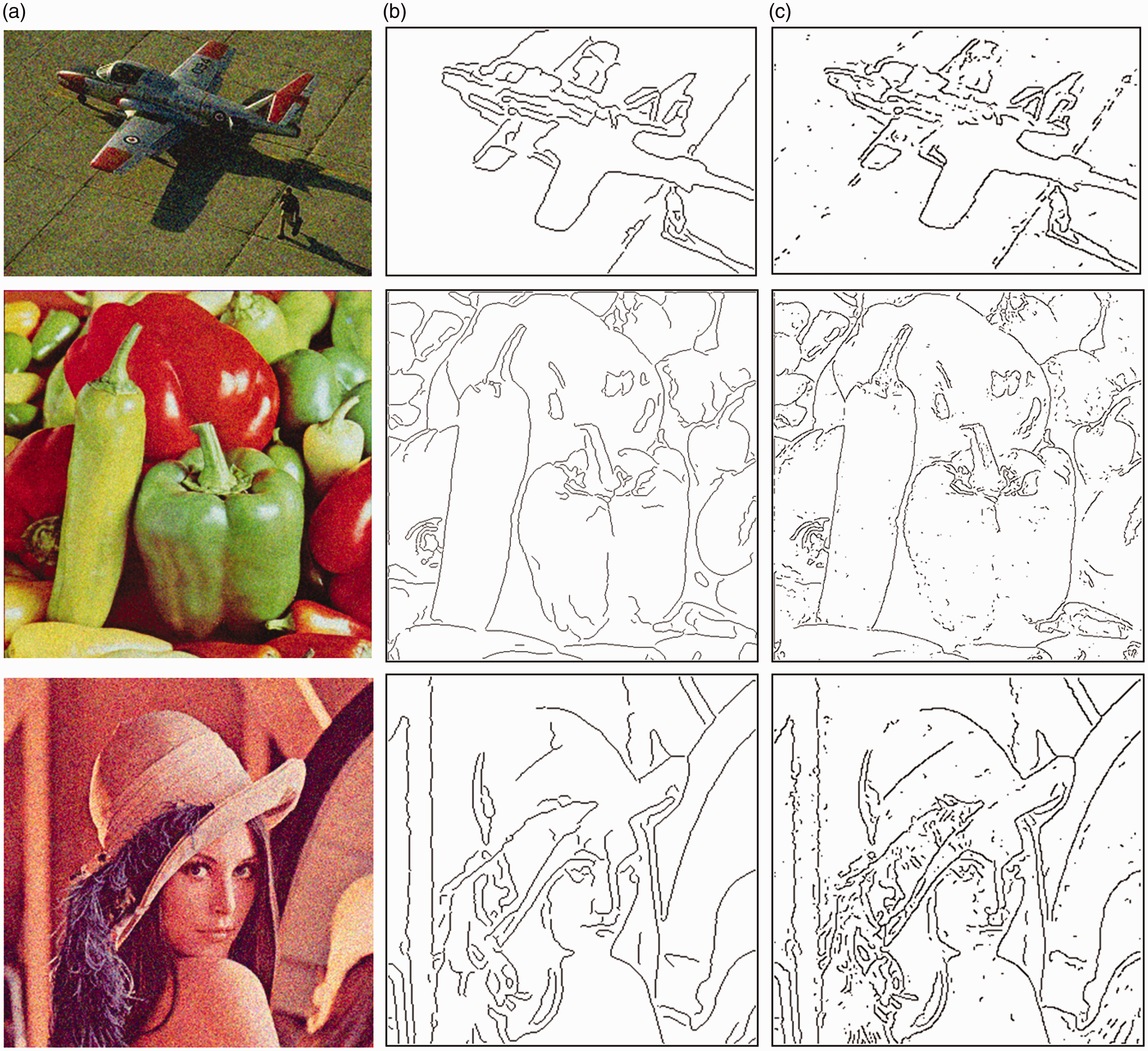
In our study, we used up to hundred different industrial images (e.g. particle images, crack images, etc.) for testing, and in this paper, six typical images are selected for the presentation of the algorithm effects, they are: three well-known images (Aircraft, Peppers and Lena) and three their noised images were used for image segmentation processing. We performed the above-mentioned modified Canny edge detector on the six images. Figure 1 shows the comparison between the results obtained using the original and modified Canny operators, where (a) to (c) shows three different original color images, the corresponding edge detection results by applying the modified Canny operator, and those using the traditional Canny operator, respectively. It is clear that the modified Canny detector can be used to accurately extract edge information and has significant advantages with respect to the suppression of noise and isolated points. In contrast, on using the traditional Canny edge detector, parts of the boundary information were lost, for example, for the edges in the bottom right part of the second image, where the objects are not identified effectively owing to noise.

Figure 1.

Comparison between the edges detected using the modified and traditional Canny operators. (a) Original image; (b) edges obtained using the modified Canny operator; (c) edges obtained using the traditional Canny operator.

To prove the robustness of the modified Canny operator, 10% random noise is added to the images shown above and the performances of the modified and traditional Canny operators are compared again. Based on our obtained results, it was observed that the traditional Canny operator retains most of the noise points, and the modified Canny operator eliminates the noise points and effectively extracts the boundary information, see Figure 2.

Figure 2.

Comparison between edges detecting using the modified and traditional Canny operators for noised images. (a) Image with 10% noise; (b) results obtained using the modified Canny operator; (c) results obtained using the traditional Canny operator.

Modified minimum spanning tree algorithm and Canny operator

The Minimum Spanning Tree (MST) algorithm proposed by Felzenszwalb involves mapping an image onto a weighted graph G(V, E), after which the image is segmented using the MST algorithm suggested by Krusal, which is based on the merging strategy. This method includes three parameters, namely σ, k and min_size, where σ is the Gaussian filter parameter; k is the key parameter of the threshold function, which is used to control the image segmentation level; and min_size is a re-merge parameter. In particular, two regions can be combined together if one region’s size in two adjacent domains is less than min_size. MST algorithm has a simple structure and it is computationally effective, however, it suffers from a few shortcomings. Therefore, we make the following improvements in terms of parameter k. Before image segmentation, in order to enhance week edges, we studied and used a fractional differential algorithm.

Fractional differential operator

Since a noisy image contains more or less weak edges which might be a part of object boundaries, no matter Canny edge detector or graph-based algorithm, the weak edge information will be ignored, and the segmentation result will be affected. In order to enhance week edges, we studied and used a fractional differential algorithm.

Generally, a two-dimensional images can be enhanced by using the first two-order differential algorithms such as edge detector Sobel, Laplacian or Canny, etc. Although these algorithms can sharpen the edges and textures, they increase noise much in some cases and are difficult to sharpen the weak edges in images. Fractional difference can partially detect the week edges and keep image noise lower. Hence, Fractional difference is suitable for the complicated images.^19,20

For an energy function ( $\mathrm{or} \mathrm{signal}{)}^{s(t)\in L^2(R)}$ , its v-order fractional differential is

$$D^{v}s(t)=D_{v}s(t)=\frac{d^{v}s(t)}{d{t}^v}$$

(1)

Then its Fourier transformation can be expressed as

$$\left(\stackrel{\wedge }{D_{v}s}\right)(\omega )={\left(i\omega \right)}^v\cdot \stackrel{\wedge }{s\left(\omega \right)}=\stackrel{\wedge }{d_v\left(\omega \right)}\stackrel{\wedge }{s\left(\omega \right)}v\in R^{+}$$

(2)

where the v order differential operator $D_v=D^v$ is a multiplicative operator of v order differential multiplier function $\stackrel{\wedge }{d\left(\omega \right)}={\left(i\omega \right)}^v$ . The filter function of the fractional order differential can be

$$\{\begin{array}{l}\stackrel{\wedge }{d\left(\omega \right)}={\left(i\omega \right)}^v=\stackrel{\wedge }{a_v\left(\omega \right)}\cdot \exp \left(i{\theta }_v\left(\omega \right)\right)=\stackrel{\wedge }{a\left(\omega \right)}\cdot \stackrel{\wedge }{p_v\left(\omega \right)}\hfill \\ \stackrel{\wedge }{a_v\left(\omega \right)}={\left|\omega \right|}^v\hfill \\ {\theta }_v\left(\omega \right)=\frac{\text{v}\pi }{2}\mathrm{sgn}\left(\omega \right)\hfill \end{array}$$

(3)

We can see from equation (3) the comparison results of the amplitude–frequency characteristic curve of the fractional order differential, the first and the second orders.

The G-L definition of fractional order differential is made based on the classical definition of studying integral order derivative in a continuous function, and the order and dimension of the calculus from integer to fraction are extended. A brief explanation is as follows:

For $\forall v\in R$ , the integral part is $[v]$ if signal $s(t)\in [a,t]\begin{array}{cc}\hspace{0.17em}& (a<t,a\in R,t\in R)\end{array}$ has to meet the condition $m+1$ < $m\in Z$ , Z presents the integer set order continuous derivative, and when $v>0$ , m is equal to $[v]$ , then we have v order derivative

$${}_{a}D{{\hspace{0.17em}}_t}^{v}s(t)=\underset{h\to 0}{\lim }{s}_h^v(t)=\underset{\mathit{nh}\to t-a}{\underset{h\to 0}{\lim }}{h}^{-v}{\displaystyle \sum _{r=0}^n{C}_r^{-v}}s(t-\mathit{rh})$$

(4)

where $C_r^{-v}=(-v)(-v+1)\cdots (-v+r-1)/r!$

If one-dimensional signal s(t) is $t\in [a,t]$ , the signal duration [a,t] is divided equally on the unit equal interval h=1 as

$$n=\left[\frac{t-a}{h}\right]\stackrel{h=1}{=}[t-a]$$

(5)

The v order fractional expression of one-dimensional signal ^s(t) is deducted as

$$\begin{array}{l}\frac{d^{v}s(t)}{d{t}^v}\approx s(t)+(-v)s(t-1)+\frac{(-v)(-v+1)}{2}s(t-2)\\ +\frac{(-v)(-v+1)(-v+2)}{6}s(t-3)+\cdots ,\\ +\frac{\Gamma (-v+1)}{n!\Gamma (-v+n+1)}s(t-n)\\ =a_{0}s(t)+a_{1}s(t-1)+a_{2}s(t-2)+a_{3}s(t-3)\\ +\cdots ,+a_{n}s(t-n)\end{array}$$

(6)

In all the n + 1 non-zero coefficient values, when the coefficient value of the first term is constant “1”, the other n non-zero coefficient values can be in the fractional order differential function. The n +1 non-zero coefficient values are in order as

$$\{\begin{array}{l}{a}_0=1\hfill \\ a_1=-v\hfill \\ a_2=(-v)(-v+1)/2=(v^2-v)/2\hfill \\ a_3=(-v)(-v+1)(-v+2)/6=(-v^3+3v^2-2v)/6\hfill \\ \begin{array}{l}{a}_4=(-v)(-v+1)(-v+2)(-v+3)/24=(v^4-6v^3+11v^2-6v)/24\\ \dots \dots \end{array}\hfill \\ a_n=\Gamma (-v+1)/n!\Gamma (-v+n+1)\hfill \end{array}$$

(7)

It can be proved that the sum of all the n + 1 non-zero coefficient values will be equal to zero, which is the main different property between the fractional order differential and the integral order differential.

If we insert the coefficients into a 5 × 5 template, the fractional differential kernel can be got as shown in the left side of equation (8), which is the Tiansi kernel, and if the kernel is presented by a fractional order, the result can be presented in the right side of equation (8).

$$\begin{array}{|ccccc|}\hline a_2& \hspace{0.17em}& a_2& \hspace{0.17em}& a_2\\ \hspace{0.17em}& a_1& a_1& a_1& \hspace{0.17em}\\ a_2& a_1& A{a}_0& a_1& a_2\\ \hspace{0.17em}& a_1& a_1& a_1& \hspace{0.17em}\\ a_2& \hspace{0.17em}& a_2& \hspace{0.17em}& a_2\\ \hline\end{array}=\begin{array}{|ccccc|}\hline (v^2-v)/2& 0& (v^2-v)/2& 0& (v^2-v)/2\\ 0& -v& -v& -v& 0\\ (v^2-v)/2& -v& 8& -v& (v^2-v)/2\\ 0& -v& -v& -v& 0\\ (v^2-v)/2& 0& (v^2-v)/2& 0& (v^2-v)/2\\ \hline\end{array}$$

(8)

If k(i,j) is for a kernel function, the sum of the coefficients or the weights in a 5 × 5 template is written as. ${\sum }_{i-2}^{i+2}{\sum }_{j-2}^{j+2}k(i,j)=-12v+4v^2=u$ . To sharpen an image, we can make ${\sum }_{i-2}^{i=2}{\sum }_{j-2}^{j+2}k(i,j)=u-12v+4v^2=1$ , the center point coefficient in a 5 × 5 kernel is u = 12v − 4v²+1, where u value is calculated on the fractional order v. In the Tiansi operator, u = Aa₀ = 8, which is a constant (see equation (8)).

In the kernel, if the coefficients of the fractional differential are calculated only based on the distances between the detecting point and its neighboring point, then a new kernel can be obtained: the coefficients (a₁, a_1-2, a₂, a_2-3, a₃, a_3-4) are got by using equations (7) and (9). In this case, there is no zero coefficient in the kernel. The values of the coefficients are computed according to the distances, for instance, when the distance is 1 pixel length, the coefficient is a₁, and when the distance is $\sqrt{2}$ pixels, the coefficient is a_1-2 as counted in equation (9). Therefore, the coefficients in the new kernel can be written as: the center point value in the kernel is w = (16v³ − 108v²+ 164v)/12 + 1.

$$\{\begin{array}{l}{a}_{1-2}=(a_1+a_2)/2=(v^2-3v)/4\hfill \\ a_{2-3}=(a_2+a_3)/2=(-v^3+6v^2-5v)/12\hfill \\ a_{3-4}=(a_3+a_4)/2=(v^4-10v^3+23v^2-14v)/48\hfill \end{array}$$

(9)

$$\begin{array}{l}\begin{array}{|c|}\hline \begin{array}{ccccc}{a}_3& a_{2-3}& a_2& a_{2-3}& a_3\\ a_{2-3}& a_{1-2}& a_1& a_{1-2}& a_{2-3}\\ a_2& a_1& A{a}_0& a_1& a_2\\ a_{2-3}& a_{1-2}& a_1& a_{1-2}& a_{2-3}\\ a_3& a_{2-3}& a_2& a_{2-3}& a_3\end{array}\\ \hline\end{array}\\ =\begin{array}{|c|}\hline \begin{array}{ccccc}(-v^3+3v^2-2v)/6& (-v^3+6v^2-5v)/12& (v^2-v)/2& (-v^3+6v^2-5v)/12& (-v^3+3v^2-2v)/6\\ (-v^3+6v^2-5v)/12& (v^2-3v)/4& -v& (v^2-3v)/4& (-v^3+6v^2-5v)/12\\ (v^2-v)/2& -v& w& -v& (v^2-v)/2\\ (-v^3+6v^2-5v)/12& (v^2-3v)/4& -v& (v^2-3v)/4& (-v^3+6v^2-5v)/12\\ (-v^3+3v^2-2v)/6& (-v^3+6v^2-5v)/12& (v^2-v)/2& (-v^3+6v^2-5v)/12& (-v^3+3v^2-2v)/6\end{array}\\ \hline\end{array}\end{array}$$

(10)

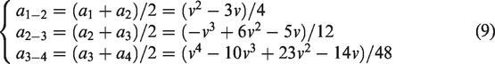
In a 5 × 5 kernel, the new kernel model is got as shown in the left side of equation (10). The coefficient computation rule is shown as in the right side of equation (10). In the above new kernel, there is no zero coefficient, the central point coefficient is w = (16v³−108v²+164v)/12 + 1, when v=0.5 or v=1.5, and w=5.75 which is closed to the central point coefficient u=6.0, not the fixed value 8 as in the traditional Tiansi kernel.

The kernel size selection is important, if it small, e.g. 3 × 3, we cannot get the good performance result, and the sharpening is rough; if it is large, e.g. more than 7 × 7, a lot of computation is needed and the result cannot be expected. Since the traditional Tiansi kernel is a 5 × 5 kernel, we also choose the new algorithm kernel size 5 × 5. As tested, when v = 0.5, the image sharpening result is the best in our case. According to the above description, the new algorithm can perform well for the week edge image sharpening and enhancement.

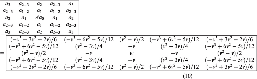
As Wu stated based on the experiments in his thesis, ²¹ when the fractional differential order v increases from 0.1 to 0.5, the weak edges will be sharpened gradually, but the noise can also be sharpened; when v is over 0.5, the noise will increase sharply. As shown in Figure 3, a simple pavement crack image with a rough surface is enhanced by different v values, when v is 0.7 or 0.8, there is a lot of noise. In our case of weak edge images with much noise, we choose v value as 0.5 to largely enhance weak edges, and the noise can be reduced by an ordinary image smooth filter such as Gaussian filter.

Figure 3.

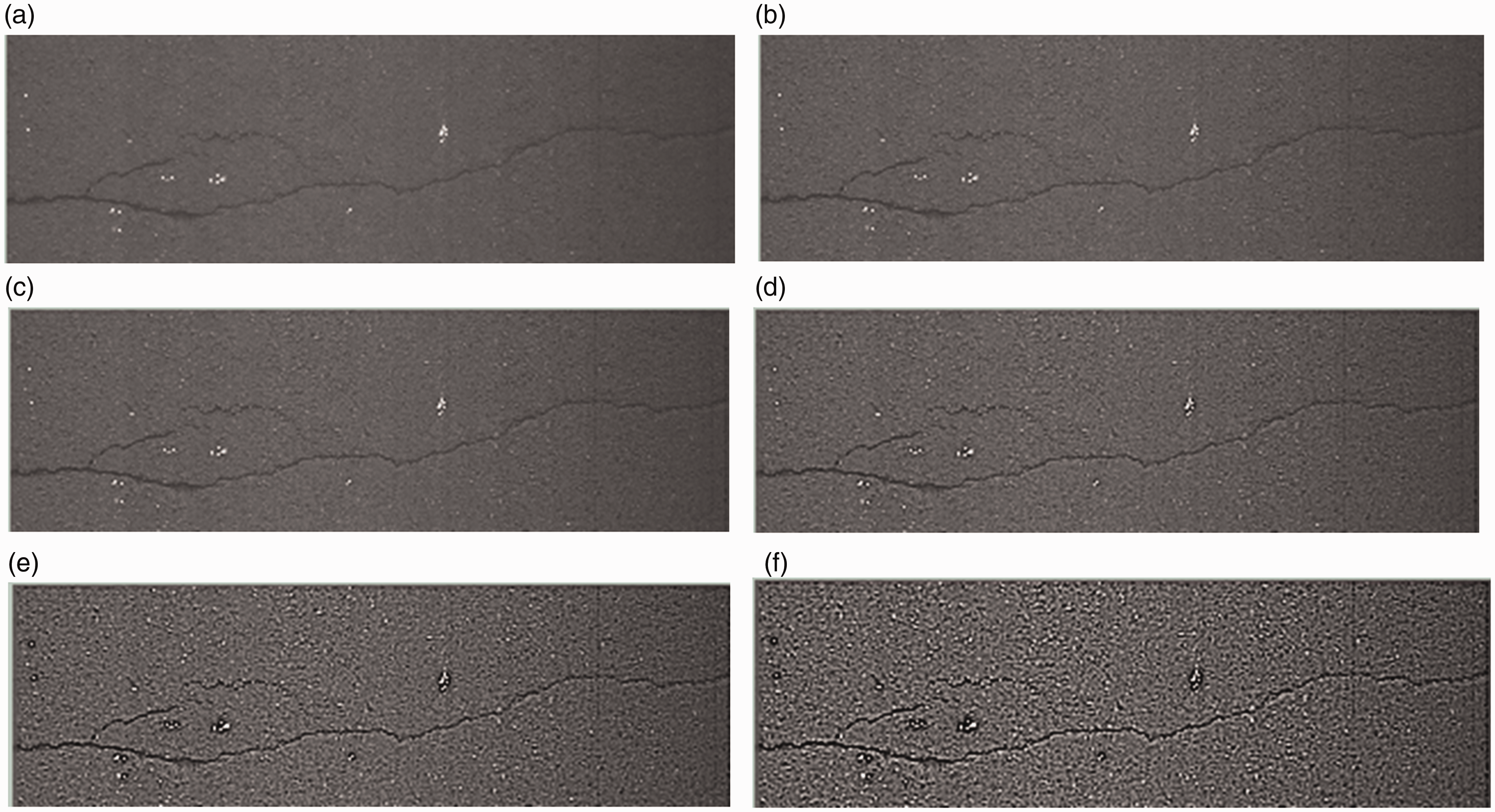
Image enhancement results of Different v. (a) Original image; (b) v = 0.1; (c) v = 0.3; (d) v = 0.5; (e) v = 0.7; (f) v = 0.8.

Improvements of minimum spanning tree algorithm

Ameliorating the difference between the intra-regional and inter-regional functions in MST

In the original form of MST, only the degree of difference in the region with maximum edge weight was represented, making it vulnerable to noise and isolated points, which consequently led to deterioration in the image segmentation results as well. To avoid this, the intra-regional differences were redefined as follows

$$\mathit{Int}\left(C\right)=1/N*{\displaystyle \sum _{e\in \mathit{MST}\left(C,E\right)}w\left(e\right)}$$

(11)

This indicates that the intra-regional difference is equal to the average value of the edge weight w(e) of MST in the region, where N is the number of edges in MST, i.e. N = | C | −1.

In the similar manner, the inter-regional differences can be defined as follows

$$\begin{array}{l}D\mathit{if}\left(C_1,C_2\right)\\ =\frac{1}{2}\left(\underset{v_i\in C_1,v_j\in C_2,\left(v_i,v_j\right)\in E}{\min }w\left(v_i,v_j\right)+\underset{v_i\in C_1,v_j\in C_2,\left(v_i,v_j\right)\in E}{\max }w\left(v_i,v_j\right)\right)\end{array}$$

(12)

Ameliorating the edge weight function

The above-mentioned improvements are aimed at the segmentation criterion. In particular, the image segmentation effect of MST algorithm primarily depends on the following two aspects: the segmentation criteria and design of the weighting function. The weighting function proposed by Felzenszwalb represents only the absolute difference between the gray scale values, without taking the spatial positions of each pixel into consideration; therefore, the weighting function of the intra-regional edge is rewritten as follows

$$w\left(v_i,v_j\right)=\mu \left(v_i,v_j\right)\left|I\left(v_i\right)-I\left(v_j\right)\right|+d\left(v_i,v_j\right)$$

(13)

where I (v_i) and I (v_j) are the gray levels of pixels v_i and v_j, respectively; furthermore, d (v_i, v_j) is defined as the Euclidean distance between v_i and v_j as follows

$$d\left(v_i,v_j\right)=\sqrt{{\left(x_i-x_j\right)}^2+{\left(y_i-y_j\right)}^2}$$

(14)

where (x_i, y_i) and (x_j, y_j) denote the coordinates of v_i and v_j, respectively. In addition, μ (v_i, v_j) is called the adjustment factor, which regulates the gray level difference and weight coefficient of the distance between two pixels; in particular, it is an adaptive two-dimensional Gaussian factor, which is defined as follows

$$\begin{array}{l}\mu \left(v_i,v_j\right)\\ =\frac{1}{{\sigma }_i{\sigma }_j\sqrt{2\pi \left(1-r^2\right)}}·\exp \{-\frac{1}{2\left(1-r^2\right)}\times [\frac{{\left(i-{\mu }_i\right)}^2}{{\sigma }_i^2}\\ -\frac{2r\left(i-{\mu }_i\right)\left(j-{\mu }_j\right)}{{\sigma }_i{\sigma }_j}+\frac{{\left(j-{\mu }_j\right)}^2}{{\sigma }_j^2}]\}\end{array}$$

(15)

where μ_i and μ_j are expected gray levels of the direction pixels; σ_i and σ_j are standard deviations of the gray levels of the direction pixels. Furthermore

$$r=\mathrm{cov}\left(i,j\right)/\sqrt{x^2+y^2}$$

(16)

$$\mathrm{cov}\left(i,j\right)=E\left(\mathit{ij}\right)-E\left(i\right)E\left(j\right)$$

(17)

For the non-associated edge with the boundary points, the edge weight function is defined as follows

$$w\left(v_i,v_j\right)={\left(\mu \left(v_i,v_j\right)\left|I\left(v_i\right)-I\left(v_j\right)\right|+d\left(v_i,v_j\right)\right)}^{\alpha },a>1$$

(18)

The advantages of above-mentioned modifications are to strengthen the algorithmic penalty for the boundary edges, which contributes to regional division. Hence, the steps of partitioning in the improved MST algorithm are as follows:

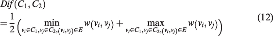
Pre-processing: Gaussian smoothing for the input image to remove noise;

Edge detection: Determining the boundary information of an image using the improved Canny operator;

Fractional differential: Using a 5 × 5 kernel sharpening week edges in the preprocessed image;

Mapping an image to graph G (V, E): Construct an 8-linked weighted graph, |V | = n, |E | = m, and then divide the edges of the weighted graph into two classes: one of the classes includes edges not associated with the edge point of the image, which are set to E₁, |E₁|=m₁, while the other class includes edges associated with the edge point of the image and are set to E₂, | E₂|=m₂, where m₁+ m₂ = m. Furthermore, the connection weights are set to w (v_i, v_j) ;

Sorting: E₁ and E₂ are arranged in the non-decreasing order separately to obtain the collection π₁ = (O₁, O₂, … , O_m1) , π₂ = (O_m1 + 1, O_m1 + 2, … , O_m) , then π = (O₁, O₂, … , O_m) ;

Initial State: Assume that the initial segmentation is S ⁰, where S ⁰ = (v₁, v₂, … , v_n), i.e. each element (vertex) of V is a single region; repeat Step 5 for q = 1, 2, … , m;

Looping: Suppose S^q−1 is the cut set after merging q−1 times, and then establish S^q from S^q−1 as follows. Let C q − 1 I and C q − 1 j be the components containing V_i and V_j, respectively, in S ^q−1; if C q − 1 i≠C q − 1 j, and Dif (C q − 1 i, C q − 1 j) ≤ min(Int (C q − 1 i)+τ (C q − 1 i), Int (C q − 1 j)+ τ (C q − 1 j)), then merge the clusters C q − 1 I and C q − 1 j to obtain S^q, else, do not merge them, i.e. S^q = S^q−1;

Merging: Return S = S^m and then deal with S ground on the re-merging mechanism;

Labeling: Assign the pixels belonging to the same region with the same color.

Output: Output the image segmentation results.

The flowchart of the above-mentioned algorithm is shown in Figure 4 where 1 (indicated in red) is the part of the algorithm for the Canny operator, while 2 (indicated in red) is that of the fractional differential and the improved graph-based algorithm.

Figure 4.

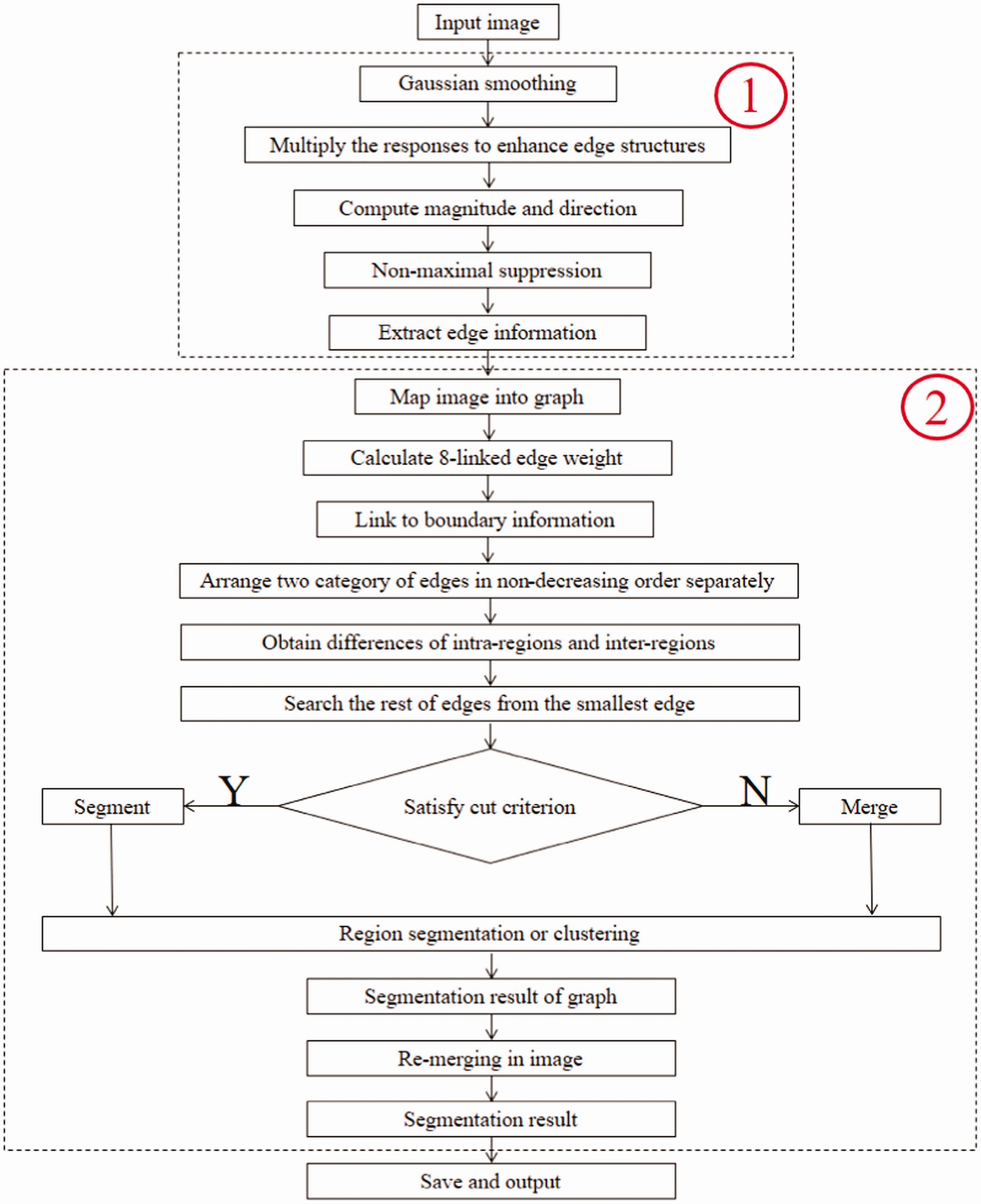
Flowchart for our proposed algorithm. In this figure, number 1 (indicted in red) is the part of the algorithm for the Canny operator, while number 2 (indicated in red) is that of the fractional differential and the improved graph-based algorithm.

Segmentation results and comparison

For comparison between different algorithms, including our proposed algorithm, we used different industrial images for experiments, where, to show the detailed information of the five algorithm results, we selected six typical images (they are three well known images: Aircraft, Peppers and Lena, and their noised images) for the testing results. The five image segmentation algorithms include the improved MST, original MST, Region merging algorithms^22,23 and Clustering and FCM algorithms^24–27 for the three original images from Figure 1. In addition, for the other three images in Figure 2, the 10% of noises are added on. And all the algorithms are tested on the three noised images. The tested results are shown in Figures 5 and 6. All of the corresponding parameters were set to be the same values in the two different graph-based algorithms. In addition, the segmentation results were shown by using different colors for the other three methods in order to allow for convenient and intuitive comparisons.

Figure 5.

Major object marking (see digital figures) in the three images in Figure 1.

Figure 6.

Segmentation results overlay the object boundaries of the manual segmentation, for the three algorithms compared in our study. (a1–a3) is for Improved algorithm; (b1–b3) is for Original graph-based algorithm; (c1–c3) is for Region merging algorithm; (d1–d3) is for Clustering algorithm; and (e1–e3) is for FCM algorithm.

In order to compare the image segmentation efficiency by different algorithms, we manually draw the object boundaries in the images, and we only marked 5–6 major objects (the objects can be seen clearly) in the images, respectively, and we take the non-marked objects as background. Since the over-segmented objects are easy to be merged together in the three images, the main problem for the image segmentation is under-segmentation in the three images. We count the number of merging between objects as OO, and the number of merging between object and back ground as OB. For in instance, in Figure 6(b1), object 1 and object 4 are merged together after image segmentation, and object 1 and object 2 are merged, so we count OO = 2; the object 1, 4, 3 merged with background (or non-marked objects), so we count OB = 3. Table 1 gives out counting results for the image segmentation efficiency by five different algorithms in Figure 6. For all the three images, Table 1 shows that the new algorithm produces less OO and OB, which means that it can have less under-segmentation problems than other algorithms.

Table 1.

Algorithm comparison for image segmentation of the three images.

Image	OO	OB	Image	OO	OB	Image	OO	OB
a1	1	0	a2	0	1	a3	1	0
b1	2	3	a2	0	2	b3	2	0
c1	2	3	c2	3	2	c3	3	2
d1	2	4	d2	5	6	d3	3	2
e1	5	5	e2	5	6	e3	4	2

Comparing the results from the five algorithms, it can be observed that our proposed algorithm can preserve more details of the images compared with the other algorithms; furthermore, it overcomes over-clustering when the parameters are set to comparatively large. As can be seen from the first row in Figure 6, because the head and top airfoil of the aircraft were misclassified as the background by the original MST algorithm, the shadow was integrated with the body of the aircraft. Clustering algorithm has the similar problem too. For Region merging algorithm, it is observed that there is the over-segmentation problem in several regions; some lines on the runway/airstrip are missing. For FCM algorithm, large parts of objects are classified into background. Anyhow, the improved MST segmentation algorithm over the other algorithms is that the new algorithm can consolidate the gradient regions of colors into one area, it can extract the detailed object information, and it has less over-segmentation and under-segmentation problems.

For the image of the peppers in the second row, the improved algorithm separately identified each pepper of the three large peppers, and the original MST algorithm and Region merging algorithm suffer from under-segmentation, especially for the large pepper on the bottom. For Clustering algorithm, the three large peppers with other parts are classified into one large object, and many small parts on right are segmented as a long shaped object, which is the under-segmentation problem. In the result of FCM, three large peppers are over-segmented, and the top-right parts are under-segmented.

Then, as can be seen in the third row, the new algorithm separated Lena’s face more clearly than the other algorithms. For the other algorithms, they suffer from under-segmentation more or less especially in the hat and face parts, and some parts, e.g. hair parts, are unclear.

For the other three images which have 10% noised in Figure 1, comparing to the new algorithm, the other four algorithms have more under-segmentation and over-segmentation problems, and are more easily affected by noise as shown in Figure 7. For example, in the first row of Figure 7, the proposed algorithm splits each part of the aircraft appropriately, compared with the segmentation results of the foreground and background obtained using the original graph-based algorithm, wherein the output is messy, and it is difficult to distinguish the different objects. Then, in the second row in Figure 7, the under-segmentation is still observed in the case of using the original MST algorithm. Furthermore, for the image in the third row, while the under-segmentation is observed, Lena’s face was segmented confusingly by utilizing the original MST algorithm. For Clustering algorithm, there is a big problem for under-segmentation; and for FCM, the over-segmentation problem is obvious. In all the three images, the results of the other algorithms are adversely affected by noise, leading to inaccurate splitting of the images into different parts. Hence, based on these observations, it can be said that the improved MST algorithm is good for preventing noise. The image segmentation results are listed in Table 2, and the new algorithm has less OO and OB, so the studied algorithm can make less under-segmentation results than the other four algorithms for this kind of noised images.

Figure 7.

Comparison of the segmentation results obtained using the five algorithms for noisy images. (a1–a3) is for Improved MST algorithm; (b1–b3) is for Original MST algorithm; (c1–c3) is for Region merging algorithm; (d1–d3) is for Clustering algorithm; and (e1–e3) is for FCM algorithm.

Table 2.

Algorithm comparison for image segmentation of the three noised images.

Image	OO	OB	Image	OO	OB	Image	OO	OB
a1	2	1	a2	1	2	a3	2	0
b1	3	3	a2	1	3	b3	2	0
c1	2	3	c2	3	4	c3	4	2
d1	2	4	d2	4	6	d3	4	5
e1	5	5	e2	4	6	e3	3	5

Moreover, for the three images, the object boundaries were manually drawn, based on the manual segmentation results, the image segmentation precision of each algorithm was calculated separately; these results were compared and are listed in Table 1. It is clear that the proposed algorithm has significant advantages in terms of the accuracy of image segmentation.

Detailed legend: For the three original images in Figure 1 and the three noised images in Figure 2, the image segmentation accuracy (comparing to manual segmentation) of each algorithm was calculated separately; these results are compared with each other and are listed in Table 3. From the figures, it is clear that the proposed image segmentation algorithm has significant advantages in terms of the accuracy of image segmentation.

Table 3.

Segmentation accuracy of the five algorithms in Figures 5 and 6, respectively.

Image/Algorithm	Aircraft (noise)	Peppers (noise)	Lena (noise)
New MST	90.9% (84.8%)	89.7% (86.7%)	90.1% (83.1%)
MST	86.9% (74.5%)	83.7% (81.5%)	86.1% (79.2%)
Region Merging	87.0% (61.6%)	84.4% (62.3%)	77.2% (65.3%)
Clustering	77.3% (65.4%)	79.2% (58.4%)	88.0% (35.8%)
FCM	74.6% (58.9%)	82.1% (65.3%)	75.5% (66.7%)

Conclusions

For the segmentation of images with much noise or/and weak edge characteristics, we proposed a novel algorithm that combines an improved Canny edge detector and an improved MST algorithm with improved Fractional differential algorithm. The new algorithm eliminates under-segmentation to some extent that is caused by over-merging using MST approach. Furthermore, by introducing the improved Canny edge detection operator for preliminary classification of pixels in an image before applying the improved MST algorithm to cluster the pixels, the effect of noise on segmentation is effectively reduced, thus improving the image segmentation accuracy by modifying the intra-regional and inter-regional difference functions and introducing the edge weight function. Since there is too may noise in an image in this study, we have to do Gaussian smoothing which can make edge weak, hence we add an improved Fractional differential algorithm to resolve the problem. Compared with the original MST, Region Merging, Clustering, and FCM algorithms, the studied algorithm has a smaller misclassification rate and the better image segmentation effect.

However, in the current work, only a preliminary study on noisy images was conducted using the proposed algorithm; nevertheless, some more issues are still needed, for example, determining the manner in which the image segmentation parameters in the improved MST algorithm can be dynamically set. These tasks will be addressed in the future study.