A comparative study of two key algorithms in multiple objective linear programming

Abstract

Multiple objective linear programming problems are solved with a variety of algorithms. While these algorithms vary in philosophy and outlook, most of them fall into two broad categories: those that are decision space-based and those that are objective space-based. This paper reports the outcome of a computational investigation of two key representative algorithms, one of each category, namely the parametric simplex algorithm which is a prominent representative of the former and the primal variant of Bensons Outer-approximation algorithm which is a prominent representative of the latter. The paper includes a procedure to compute the most preferred nondominated point which is an important feature in the implementation of these algorithms and their comparison. Computational and comparative results on problem instances ranging from small to medium and large are provided.

Introduction

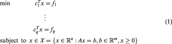
Multiple objective linear programming (MOLP) is a branch of multiple criteria decision making (MCDM)^32,33 that seeks to optimize two or more linear objective functions subject to linear constraints. Indeed, many real-world decision-making problems involve more than one objective function and can be formulated as MOLP problems. MOLP models have been widely applied in many fields of human endeavour such as science, engineering and management and have become a useful tool in decision making. An MOLP problem can be expressed as

$$\begin{array}{l}\text{min}{c}_1^{T}x=f_1\\ ⋮\\ c_q^{T}x=f_q\\ \text{subject}\text{to}x\in X=\left\{x\in {\mathbb{ℝ}}^n:\mathit{Ax}=b,b\in {\mathbb{ℝ}}^m,x\ge 0\right\}\end{array}$$

(1)

or alternatively as a linear vector optimization problem

$$\begin{array}{l}\text{min}\mathit{Cx}\\ \text{subject}\text{to}\mathit{Ax}=b\\ x\ge 0\end{array}$$

(2)

where C is a q × n criterion matrix consisting of the rows $c_k,k=1,\dots ,q$ , A is an m × n constraint matrix and $b\in {\mathbb{ℝ}}^m$ is the right hand side vector. The feasible set in the decision space is $X=\left\{x\in {\mathbb{ℝ}}^n:\mathit{Ax}=b,x\ge 0\right\}$ , and in the objective space, it is $Y=\left\{\mathit{Cx}:x\in X\right\}$ . The set Y is also referred to as the image of X. The upper image is defined as Y +  ${\mathbb{ℝ}}_{+}^q$ .

In practice, MOLP is typically solved by the Decision Maker (DM) with the support of the analyst looking for a most preferred (best) solution in the feasible region X. This is because optimizing all the objective functions simultaneously is not possible due to their conflicting nature. Consequently, the concept of optimality is replaced with that of efficiency. The purpose of MOLP is to obtain either all the efficient or nondominated points or a subset of either or a most preferred point depending on the purpose for which it is needed.

An efficient solution of an MOLP problem is a solution that cannot improve any of the objective functions without deteriorating at least one of the other objectives. A weakly efficient solution is one that no other solution can improve all the objective functions simultaneously.

A nondominated point in the objective space is the image of an efficient solution in the decision space, and the set of all nondominated points forms the nondominated set. Let $\widehat{x}\in X$ be a feasible solution of equation (2) and let $\widehat{y}=C\widehat{x}$ :

$\widehat{x}$ is called efficient if there is no $x\in X$ , such that $\mathit{Cx}\le C\widehat{x}$ and $\mathit{Cx}\ne C\widehat{x}$ ; correspondingly, $\widehat{y}=C\widehat{x}$ is called nondominated.

$\widehat{x}$ is called weakly efficient if there is no $x\in X$ , such that $\mathit{Cx}<C\widehat{x}$ ; and $\widehat{y}=C\widehat{x}$ is called weakly nondominated. ¹

The set of all efficient solutions and the set of all weakly efficient solutions of equation (2) are denoted by X_E and X_WE, respectively. The sets $Y_N=\{\mathit{Cx}:x\in X_E\}$ and $Y_{\mathit{WN}}=\{\mathit{Cx}:x\in X_{\mathit{WE}}\}$ are the nondominated and weakly nondominated sets in the objective space of equation (2), respectively.

The nondominated faces in the objective space of a given problem constitute the nondominated frontier, and the efficient faces in the decision space of the problem constitute the efficient frontier.

Robustness of method can be defined in different ways, in terms of computing efficiency or the ability of a method to solve problems depending on the researcher. In this paper, we consider it as the ability of a method to solve all problems (both simple and difficult).

The ideal objective point $y^{*}$ is the minimum criterion values over the efficient set X_E. The ideal objective values are easy to obtain by simply minimizing each objective function individually over the feasible region X. ²

MOLP has been an active area of research since the 1960s. During this period, various algorithms have been developed for generating either the entire efficient or nondominated set, or a subset of it, or a most preferred efficient or nondominated point for the problem. Most of these approaches are decision space-based. However, objective space-based methods are becoming more and more prominent.

In this paper, we are concerned with the state-of-the-art technology for MOLP. We are interested in a detailed comparison of the recently introduced parametric simplex algorithm (PSA) of Rudloff et al. ³ with the primal variant of Benson’s ⁴ outer-approximation algorithm (BOA) which is an objective space-based method. It has been noted by Benson ⁴ that, in practice, the DM prefers to base his or her choice of a most preferred (best) solution on the nondominated points. To achieve this comparison, we shall act here as the DM and choose a most preferred nondominated point (MPNP) whose components are as close as possible to an unattainable ideal objective point from the nondominated set returned by PSA to compare with a MPNP returned by BOA. These two algorithms are based on the same solution concept introduced by Löhne. ⁵ The algorithms will be compared comprehensively on a series of existing test problems.

One of the key issues in MOLP is computing the MPNP’s. We give a detailed procedure for the purpose here which allows us to carry out the comparison.

This paper is organized as follows: ‘Motivation’ section is the motivation. ‘Literature review’ section is a review of the related literature which centres on the parametric simplex and the objective space-based method that is BOA. We present PSA in ‘The parametric simplex algorithm’ section. ‘Scalarization techniques’ section discusses two scalarization techniques. BOA is presented in ‘Benson’s outer-approximation algorithm’ section. ‘Selection of the MPNP’ section discusses the selection of an MPNP. Detailed numerical experiments are presented in ‘Experimental results’ section to compare the quality of a MPNP, robustness and computing efficiency of the two algorithms. The results are summarized in the ‘Summary of results’ section. Finally, a conclusion is drawn in ‘Conclusion’ section.

Motivation

These two algorithms are similar in output but different in philosophy since one of them, BOA, is an objective space-based search algorithm, while PSA is a decision space-based algorithm. They are prominent examples of MOLP algorithms. Unfortunately, there is no empirical evidence in the literature, as far as we can tell, that separates them in terms of robustness and the quality of a MPNP they returned. This paper intends to fill this gap. It considers all available test problems ranging from small size to large size and solves them with Matlab implementations of the two algorithms on the same machine. The extensive results are recorded and discussed. It is hoped that these results would be a valuable guideline for the potential users to choose between the two depending on the problems they have to solve. It is also important to add that a comprehensive review of existing work is included. This puts the work well in context and saves the reader the need to consult much of the literature on the topic. We shall dwell more on robustness and quality of a MPNP returned by these algorithms using existing and realistic instances.

Note that to the best of our knowledge, no one tested these algorithms as extensively as we have done here in terms of the size and variety of problems.

The PSA of Rudloff et al. ³ works in the decision space and does not intend to find the set of all efficient extreme points of the problem; rather it finds a solution based on the idea of Löhne. ⁵ That is, it finds a subset of efficient extreme points and directions that allows to generate the whole efficient frontier and also returns the corresponding nondominated points and directions. BOA, on the other hand, works in the objective space to find the set of all nondominated points as well as directions of the problem.

Literature review

MOLP algorithms using a parametric programming approach have been widely studied in the last five decades. The first parametric programming approach to MOLP appears to be due to Schönfeld. ⁶ The author presented an algorithm for the enumeration of efficient solutions of the problem using parametric programming. Geoffrion ⁷ presented a bicriterion parametric linear programming algorithm to solve the problem. It was noted that solutions are not extreme points of the feasible region, pointing to the fact that one should not rely only on algorithms that consider extreme point solutions as in ordinary LP.

Evans and Steuer ⁸ introduced MSA for finding all the efficient extreme points and unbounded efficient edges for MOLPs. The algorithm first establishes that the problem is feasible and has efficient solutions. This is done by solving an auxiliary LP and two weighted sum LPs to find an initial efficient basis. Thereafter, it generates efficient bases by moving from one efficient extreme point to adjacent efficient extreme points until all the efficient extreme points have been found. The efficient extreme points are obtained using a test problem that determines the pivots that lead to them.

Zeleny ⁹ extended the approach of Geoffrion ⁷ to solve problems with more than two objectives. He decomposes the parametric space into finite subspaces that provide a set of optimal weights corresponding to extreme point solutions. It was noted that the approach might be inefficient for degenerate problems as two or more bases may be associated with the same extreme point. The vertices are tested for efficiency as soon as they are generated by solving an LP that determines the efficiency of such vertices.

Yu and Zeleny ¹⁰ presented two basic forms of parametric linear programming approaches and their computational procedures for computing the efficient set; the direct decomposition of the parametric space that was earlier introduced in Zeleny ⁹ and the indirect algebraic method. Based on a numerical experiment, the indirect algebraic method outperforms the direct decomposition method.

A parametric linear programming algorithm for generating the set of efficient vertices and higher-dimensional faces of the problem was presented by Gal. ¹¹ In this procedure, efficient extreme points are generated through the use of an auxiliary problem which itself is an ordinary LP. The algorithm also determines higher-dimensional efficient faces for degenerate problems which were only discussed in Zeleny ⁹ but not solved. The efficient faces are generated following a bottom-up search strategy, that is, they are generated based on the information provided by the efficient extreme points.

Steuer ¹² applied the MSA of Evans and Steuer ⁸ to parametric MOLP problems. Different methods for obtaining an initial efficient basis as well as different LP test problems were also presented. Similarly, Ehrgott ¹ used this MSA variant to solve parametric MOLP problems.

A modification of the PSA for single objective LP to solve bounded bicriterion LP problems was presented by Ruszczyński and Vanderbei. ¹³ The approach was applied to a large mean-risk portfolio optimization problem for which the nondominated portfolios were generated.

Ehrgott et al. ¹⁴ introduced a primal-dual simplex algorithm for bounded problems. This algorithm finds a subset of efficient solutions that are enough to generate the whole efficient frontier. The algorithm starts with a coarse partitioning of the weight space which continues in each iteration as well as solves a costly LP in each iteration. A vertex enumeration is then performed in the last step to obtain efficient solutions. Numerical illustrations show the applicability of the algorithm.

Recently, Rudloff et al. ³ presented a PSA for the problem. The algorithm is a generalization of the algorithm of Ruszczyński and Vanderbei ¹⁴ and is similar to that of Ehrgott et al. ¹⁴ It works for any dimension, solves bounded and unbounded problems (unlike that of Ehrgott et al. ¹⁴ and Ruszczyński and Vanderbei ¹³ ) and does not find all the efficient solutions just like that of Ehrgott et al. ¹⁴ Instead, it finds a solution based on the idea of Löhne, ⁵ i.e. a subset of efficient extreme points and directions that allows to generate the whole efficient frontier. This is the so-called PSA. It was compared with a version of BOA in Hamel et al. ¹⁵ and MSA of Evans and Steuer ⁸ using small MOLP instances which were randomly generated with three and four objectives and up to 50 variables and constraints. The numerical results show that the proposed algorithm outperforms Benson’s algorithm for non-degenerate problems. However, Benson’s algorithm is better for highly degenerate problems. PSA was also found to be computationally more efficient than the algorithm of Evans and Steuer. ¹⁵ This comparison only focused on computing efficiency. Here, apart from computing efficiency, we will also compare the robustness and quality of MPNP’s returned by these two methods using existing and realistic MOLP instances.

Due to the various difficulties arising from solving MOLP problems in the decision space (such as having different efficient solutions that map onto the same point in the objective space), efforts were made to look at the possibility of solving them in the objective space.

Benson, ⁴ who presented a detailed account of decision space approaches, proposed an algorithm for generating the set of all nondominated points in the objective space. This is the so-called BOA. According to him, this algorithm is the first of its kind. Computational results suggest that the objective space-based approach is better than the decision space-based one. A further analysis of the objective space-based algorithm was presented in Benson. ¹⁶ This outer approximation algorithm also generates the set of all weakly nondominated points, thereby enhancing the usefulness of the algorithm as a decision aid.

Another of Benson’s ¹⁷ suggestions is a hybrid approach for solving the problem in the objective space. The approach partitions the objective space into simplices that lie in each face so as to generate the set of nondominated points. This idea was earlier presented in Ban. ¹⁸ The algorithm is quite similar to that in Benson. ⁴ The difference is in the manner in which the nondominated vertices are found. While a vertex enumeration procedure is employed in Benson, ⁴ a simplicial partitioning technique is used in the latter.

In Shao and Ehrgott, ¹⁹ a modification of the algorithm of Benson ⁴ was presented. While in Benson, ⁴ a bisection method that requires the solution of many LPs in one step is required; here, solving one LP achieves the desired effect and in the process improves computation time. Shao and Ehrgott ²⁰ proposed an approximate dual variant of the algorithm of Benson ⁴ for obtaining approximate nondominated points of the problem. The proposed algorithm was applied to the beam intensity optimization problem of radio therapy treatment planning for which approximate nondominated points were obtained. Numerical testing shows that the approach is faster than solving the primal directly.

The explicit form of the algorithm of Benson ⁴ as modified by Shao and Ehrgott ¹⁹ is presented in Löhne. ⁵ This version solves two LPs in each iteration during the process of obtaining nondominated points and is extended to unbounded problems. Löhne ²¹ developed a Matlab implementation of this algorithm called BENSOLVE-1.2 for computing all the nondominated points and directions (unbounded nondominated edges) of the problem.

Csirmaz ²² presented an improved version of the algorithm of Benson ⁴ that solves one LP and a vertex enumeration problem in each iteration. While in Benson, ⁴ solving two LPs to determine a unique boundary point and a supporting hyperplane of the image is required in two steps; here, the two steps are merged and solving only one LP does both tasks and improves computation time. The algorithm was used to generate all the nondominated vertices of the polytope defined by a set of Shannon inequalities on four random variables so as to map their entropy region. Numerical testing shows the applicability of the approach to medium and large instances with 3 and 10 objectives and up to 5772 variables and 635 constraints.

Hamel et al. ¹⁵ introduced new versions and extensions of the algorithm of Benson. ⁴ The primal and dual variants of the algorithm solve only one LP problem in each iteration and is extended to pointed solid polyhedral ordering cones. Tests reveal a reduction in computation time. Similarly, Löhne et al. ²³ extended the primal and dual variants of this algorithm to solve convex vector optimization problems approximately in the objective space.

Based on our review of the topic, it was observed that no comparison of robustness and quality of a MPNP chosen from the nondominated set returned by PSA with the MPNP chosen from the nondominated set returned by BOA has been carried out. We intend to fill this gap here.

The parametric simplex algorithm

The PSA of Rudloff et al. ³ is one of the current solution approaches for MOLP. It can be viewed as a variant of the algorithm of Evans and Steuer, ⁸ with a similar structure. It is different in the sense that it does not find all the efficient extreme points and unbounded efficient edges (extreme rays) as is being done in Evans and Steuer. ⁸ As mentioned earlier, the algorithm works in the decision space and finds a solution based on the idea of Löhne; ⁵ i.e., it finds a finite subset of efficient extreme points and directions that allows to generate the whole efficient frontier. The algorithm is initialized by solving an LP to find a weight vector, such that the weighted sum problem using this weight vector yields an optimal solution. The corresponding optimal dictionary (containing basic and nonbasic variables) is used to construct an initial dictionary D⁰ and an index set of entering variables $J^{D^0}$ . The optimal solution is then used as an initial efficient basic feasible solution x⁰. Its implementation stores a set of Boundary Dictionaries (BD) containing dictionaries that are not yet visited and a set of Visited Dictionaries (VD) that contains dictionaries that are already visited. At each iteration, the algorithm moves from one dictionary to another, collecting their basic solutions into a set of efficient solutions $\overline{X}$ for output until all the dictionaries are visited. More specifically, the algorithm performs pivoting for only one leaving variable among the set of all possible leaving variables and picks only one entering variable, thereby making it computationally efficient. In addition, rather than solving a vertex enumeration problem which is more costlier as is being done in Benson, ⁴ the algorithm finds a set of parameters that guarantees the efficiency of the current vertex and eliminates the redundant inequalities thereof. This is done by solving a parametrized LP to check if an inequality is defining or redundant; if redundant, it would be eliminated which also improves the computation time. For unbounded problems where there is no leaving variable for an entering variable, a corresponding homogenous problem is solved, and the solution found forms the extreme directions of the problem. When all the dictionaries are visited, the algorithm stops and returns the set of efficient extreme points $\overline{X}$ and directions ${\overline{X}}^h$ as well as the corresponding nondominated vertices $\overline{Y}$ and directions ${\overline{Y}}^h$ of the problem. Before we describe the pseudo-code form of PSA, we first explain the used notation.

Notation

A, b, C

problem data

B

the set of basic variables

BD

the set of boundary dictionaries

D⁰

the initial dictionary

$E^{D^0}$

the set of explored pivots for the initial dictionary

J^D

the index set of entering variables

$J^{D^0}$

an initial index set of entering variables

N

the set of nonbasic variables

R

the recession cone of the image

x ⁰

an initial efficient basic feasible solution corresponding to the initial dictionary

The indices i, j correspond to basic variable $x_i\in B$ and nonbasic variable $x_j\in N$ , respectively

$B^{-1}$

the inverse of the basic matrix

$\overline{D}$

the new dictionary

E^D

the set of explored pivots for the current dictionary

$E^{\overline{D}}$

the set of all explored pivots of the new dictionary $\overline{D}$

$P^T[{\overline{X}}^h]$

the image of the direction

VD

the set of visited dictionaries

$\overline{x}$

the basic feasible solution for the new dictionary $\overline{D}$

x^h

a direction of recession in the decision space

$\overline{X}$

the set of efficient extreme points in the decision space

${\overline{X}}^h$

the set of extreme directions in the decision space

$\overline{Y}$

the set of all nondominated vertices in the objective space

${\overline{Y}}^h$

the set of extreme directions in the objective space

$-Z_N^T{e}^j$

a direction in the objective space

Algorithm 1

Parametric simplex algorithm ³

0: Input: A, b, C

1. Initialize: Find D⁰ $\mathit{and}\mathit{the}\mathit{index}\mathit{set}\mathit{of}\mathit{entering}$ variables $J^{D^0}$ ;

     $\mathit{BD}\leftarrow \left\{D^0\right\}$ , $\overline{X}\leftarrow \left\{x^0\right\},\overline{Y^h}\leftarrow \varnothing$ , $\mathit{VS}\leftarrow \varnothing$ , ${\overline{X}}^h\leftarrow \varnothing$ , $E^{D^0}\leftarrow \varnothing$ , $R\leftarrow \varnothing .$

2. while $\mathit{BD}\ne \varnothing$ do

3.   $\mathit{Let}D\in \mathit{BD}\mathit{with}\mathit{nonbasic}\mathit{variables}N\mathit{and}$ $\mathit{index}\mathit{set}\mathit{of}\mathit{entering}\mathit{variables}{J}^D;$

4.   $\mathbf{for}j\in J^D$ do

5.    $\mathit{Let}{x}_j\mathit{be}\mathit{the}\mathit{entering}\mathit{variable}$ ;

6.    $\mathbf{if}{B}^{-1}N{e}^j\le 0$ then

7.     $\mathit{Let}{x}^h\mathit{be}\mathit{such}\mathit{that}{x}_B^h=-B^{-1}N{e}^j$ $\mathit{and}{x}_N^h=e^j$ ;

8.     ${\overline{X}}^h\leftarrow {\overline{X}}^h\cup \left\{x^h\right\}$

9.     ${\overline{Y}}^h\leftarrow P^T[{\overline{X}}^h]\cup \{-Z_N^T{e}^j\}$

10.   else

11.      $\mathit{Pick}i\in \mathit{argmi}{n}_{i\in B,{(B^{-1}N)}_{\mathit{ij}}>0}\frac{{(B^{-1}b)}_i}{{(B^{-1}N)}_{\mathit{ij}}}$ ;

12.      $\mathbf{if}(j,i)\cancel{\in }{E}^D$ then

13.       $\mathit{Perform}\mathit{the}\mathit{pivot}\mathit{with}\mathit{entering}$ $\mathit{variable}{x}_j\mathit{and}\mathit{leaving}\mathit{variable }{x}_i$ ;

14.       $\mathit{Call}\mathit{the}\mathit{new}\mathit{dictionary}\overline{D}\mathit{with}$ $\mathit{nonbasic}\mathit{variables}\overline{N}=N\cup \left\{i\right\}\backslash \left\{j\right\}$ ;

15.        $\mathbf{if}\overline{D}\cancel{\in }\mathit{VS}$ then

16.         $\mathbf{if}\overline{D}\in \mathit{BD}$ then

17.         $E^{\overline{D}}\leftarrow E^{\overline{D}}\cup \{(i,j)\}$ ;

18.        else

19.          $\mathit{Let}\overline{x}\mathit{be}\mathit{the}\mathit{basic}\mathit{solution}$ $\mathit{for}\overline{D}$ ;

20.          $\overline{X}\leftarrow \overline{X}\cup \left\{\overline{x}\right\}$ ;

21.          $\overline{Y}\leftarrow P^T[\overline{X}]\cup \left\{P^T\overline{x}\right\}$ ;

22.         $\mathit{Compute}\mathit{the}\mathit{index}\mathit{set}\mathit{of}$ $\mathit{entering}\mathit{variables}{J}^{\overline{D}}\mathit{of}\overline{D}$ ;

23.          $\mathit{Let}{E}^{\overline{D}}=\{(i,j)\}$ ;

24.          $\mathit{BD}\leftarrow \mathit{BD}\cup \left\{\overline{D}\right\}$ ;

25.       endif

26.      endif

27.     endif

28.    endif

29.  endfor

30.   $\mathit{VS}\leftarrow \mathit{VS}\cup \left\{D\right\}$ , $\mathit{BD}\leftarrow \mathit{BD}\backslash \left\{D\right\}$

31. endwhile

32. Output: $(\overline{X},\overline{X^h}):\mathit{Set}\mathit{of}\mathit{Efficient}\mathit{solutions}\mathit{and}$ $\mathit{directions};$ $(\overline{Y},\overline{Y^h}):\mathit{Nondominated}\mathit{set}\mathit{and}$ directions.

Illustration of PSA

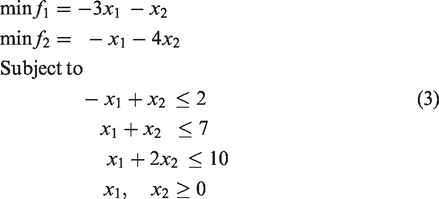
We consider the following MOLP adapted from Alves et al., ²⁴ which we solved using a Matlab implementation of PSA

$$\begin{array}{l}\text{min}{f}_1=-3x_1-x_2\\ \text{min}{f}_2=-x_1-4x_2\\ \text{Subject}\text{to}\\ -x_1+x_2\le 2\\ x_1+x_2\le 7\\ x_1+2x_2\le 10\\ x_1,x_2\ge 0\end{array}$$

(3)

The efficient extreme points found are $x^1={(2.0,4.0)}^T,x^2={(4.0,3.0)}^T$ and $x^3={(7.0,0.0)}^T$ . The corresponding nondominated points are $f^1={(-10.0,-18.0)}^T,f^2={(-15.0,-16.0)}^T$ and $f^3={(-21.0,-7.0)}^T$ , respectively, where $x^1={(x_1^1,x_2^1)}^T,x^2={(x_1^2,x_2^2)}^T,x^3={(x_1^3,x_2^3)}^T\in X_E$ and $f^1={(f_1^1,f_2^1)}^T,f^2={(f_1^2,f_2^2)}^T,f^3={(f_1^3,f_2^3)}^T$ $\in Y_N$ . The feasible region in the decision space is shown in Figure 1.

Figure 1.

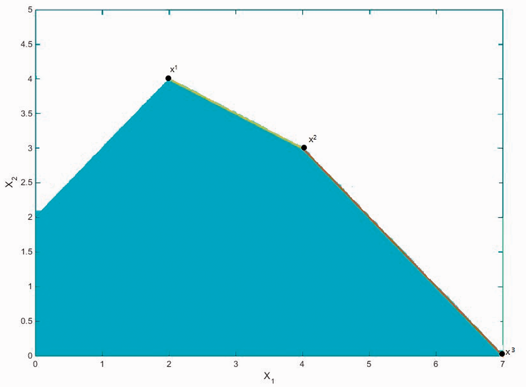
Efficient edges joining the three points in the decision space.

Scalarization techniques

Before presenting BOA, we first present two basic scalarization methods that play an important role in its implementation. These methods are weighted sum scalarization and translative or scalarization by a reference variable. As noted in Löhne, ⁵ scalarization is one of the most important techniques used in MOLP.

In the weighted sum method, a new objective function based on the q-linear objectives is obtained by assigning non-negative weights $w_i\in {\mathbb{ℝ}}^q$ to each of the objectives. The weighted sum of the objectives is ${\sum }_{i=1}^q{w}_i{c}_{i}x=w^{T}Cx.$ For each vector $w\in {\mathbb{ℝ}}^q,w\ge 0$ , we obtain a scalar linear program

$$\text{min}{w}^{T}Cx\text{subject}\text{to}\mathit{Ax}\ge b{P}_1(w)$$

The weights are usually normalized, so that $e^{T}w=1$ , with $e^T=(1,\dots ,1)$ . The dual of $P_1(w)$ is

$$\text{max}{b}^{T}u\text{subject}\text{to}\{\begin{array}{cc}{A}^{T}u=C^{T}w& \hspace{0.17em}\\ u\ge 0& D_1(w)\end{array}$$

In the method of scalarization by a reference variable, the q objectives are associated to a common reference variable z, and the ith objective is restrained from being larger than the reference variable and a fixed real number y_i, that is $c_{1}x\le y_1+z$ , $c_{2}x\le y_2+z$ , …, $c_{q}x\le y_q+z$ .

The reference variable z is the objective function that has to be minimized. By setting $e={(1,\dots ,1)}^T$ , we obtain for each vector $y\in {\mathbb{ℝ}}^q$ the scalar linear program

$$\text{min}\text{z}\text{subject}\text{to}\{\begin{array}{cc}\mathit{\text{Ax}}\ge \mathit{\text{b}}& \hspace{0.17em}\\ \mathit{\text{Cx-ze}}\le \mathit{\text{y}}\text{.}& {\mathit{\text{P}}}_{\text{2}}(\mathit{\text{y}})\end{array}$$

The dual program is

$$\text{max}{b}^{T}u-y^{T}w\text{subject}\text{to}\{\begin{array}{l}{A}^{T}u-C^{T}w=0\hspace{0.17em}\hfill \\ e^{T}w=1\hspace{0.17em}\hfill \\ (u,w)\ge 0.D_2(y)\hfill \end{array}$$

The above two scalarization techniques are fundamental for the implementation of BOA which is discussed in the next section. ⁵

Benson’s outer-approximation algorithm

This version of BOA is due to Shao and Ehrgott. ¹⁹ It can be found in Löhne. ⁵ It works in the objective space of the problem and returns the set of all nondominated points and extreme directions. The algorithm can be regarded as a primal-dual method because it also solves the dual problem. But here, we are only concerned with the solution of the primal. The algorithm first constructs an initial polyhedron Y₀ (outer approximation) containing the upper image Y in the objective space and an interior point $\widehat{p}$ of the image is determined by solving $P_1(w)$ . The inequality representation of the outer approximation is also determined by solving $D_1(w)$ . The algorithm constructs a sequence of decreasing polytope $Y_0\supseteq Y_1\supseteq \dots \supseteq Y_k=Y$ . The vertices of each polytope Y_k as well as inequality representation (facets) are stored in each iteration. Then, for each vertex v of the polytope, the algorithm checks if the vertex is on the boundary of Y. If the vertices are on it, the problem is solved. The external vertices of Y are among the vertices of Y_k. Otherwise, for any vertex v of Y_k that is not on the boundary of Y, the algorithm connects this vertex to the interior point $\widehat{p}$ and finds the intersection y of this line with the boundary of Y by solving $P_2(y)$ . Then a supporting hyperplane adjacent to y is constructed by solving $D_2(y)$ . This hyperplane is added to Y_k to provide a smaller approximation. The algorithm is repeated in the same way until the vertices of Y_k coincide with the boundary of Y. The algorithm returns the set of vertices on the boundary of Y as the nondominated set $\overline{Y}$ and directions $\overline{Y^h}$ of the problem. The notation used in the pseudo-code of BOA is as follows.

Notation

A, b, C

problem data

$D^{*h}$

the homogeneous dual problem;

k

the iteration counter

$\widehat{p}$

an interior point;

P_h

the homogeneous problem

R(v)

the LP that finds the unique value δ

$\overline{T}$

a set of solutions of the dual problem

${\overline{T}}^h$

the solution of the homogeneous dual problem

$Y_k^d$

the inequality representation of the current polytope

$Y_k^p$

the representation by vertices

$(\widehat{y},z)$

an optimal solution to $P_2(y)$

$\delta (0<\delta <1)$

a unique value that determines the intersection or boundary point y

The command $\mathit{solve}()$ solves an LP

$\mathit{vert}()$

returns the vertices of a polytope Y_k

$\overline{Y}$

the set of nondominated vertices

$({\overline{Y}}^h)$

the set of extreme directions

Algorithm 2

Benson’s outer-approximation algorithm ⁵

0: Input: $A,b,C:\mathit{Problem}\mathit{data}$

     $a\mathit{solution}(\{0\},{\overline{Y}}^h)\mathit{to}{P}^h$ ;

     $a\mathit{solution}{\overline{T}}^h\mathit{to}{D}^{*h}$ ;

1. Initialize: $\widehat{p}\leftarrow \mathit{P}(\mathit{solve}(P_1(0)))+e$ ;

2.      $\overline{T}\leftarrow \{(\mathit{solve}(D_1(w)),w)|(u,w)\in {\overline{T}}^h\}$ ;

3.  $\mathbf{while}z=0$ do

4.     $Y_k^d\leftarrow \{D^{*}(u,w)|(u,w)\in \overline{T}\}$ ;

5.     $Y_k^p\leftarrow \mathit{vert}(Y^d)$ ;

6.     $\overline{Y}\leftarrow \varnothing$ ;

7.     $\mathbf{for}i=1\mathit{to}\left|Y^p\right|$ do

8.      $v\leftarrow Y_k^p[i]$ ;

9.      $(\widehat{y},z)\leftarrow \mathit{solve}(P_2(y))$ ;

10.      $\overline{Y}\leftarrow \overline{Y}\cup \left\{\widehat{y}\right\}$ ;

11.      $\mathbf{if}z\ne 0$ then

12.       $(x,\delta )\leftarrow \mathit{solve}(R(v)),(0<\delta <1)$ ;

13.       $y\leftarrow \delta v+(1-\delta )\widehat{p}$ ;

14.       $(u,w)\leftarrow \mathit{solve}(D_2(y))$ ;

15.       $\overline{T}\leftarrow \overline{T}\cup \{(u,w)\}$ ;

16.    endif;

17.   endfor;

18. endwhile

19. Output: $(\overline{Y},\overline{Y^h}):\mathit{Nondominated}\mathit{set}\mathit{and}$ directions;

      $\overline{T}:a\mathit{solution}\mathit{to}\mathit{dual}.$

Illustration of BOA

Consider again Problem 3 of ‘Illustration of PSA’ section. The nondominated points found by Algorithm 2 are $f^1={(-21.0,-7.0)}^T,f^2={(-15.0,-16.0)}^T$ and $f^3={(-10.0,-18.0)}^T$ , respectively. These nondominated points are shown in Figure 2.

Figure 2.

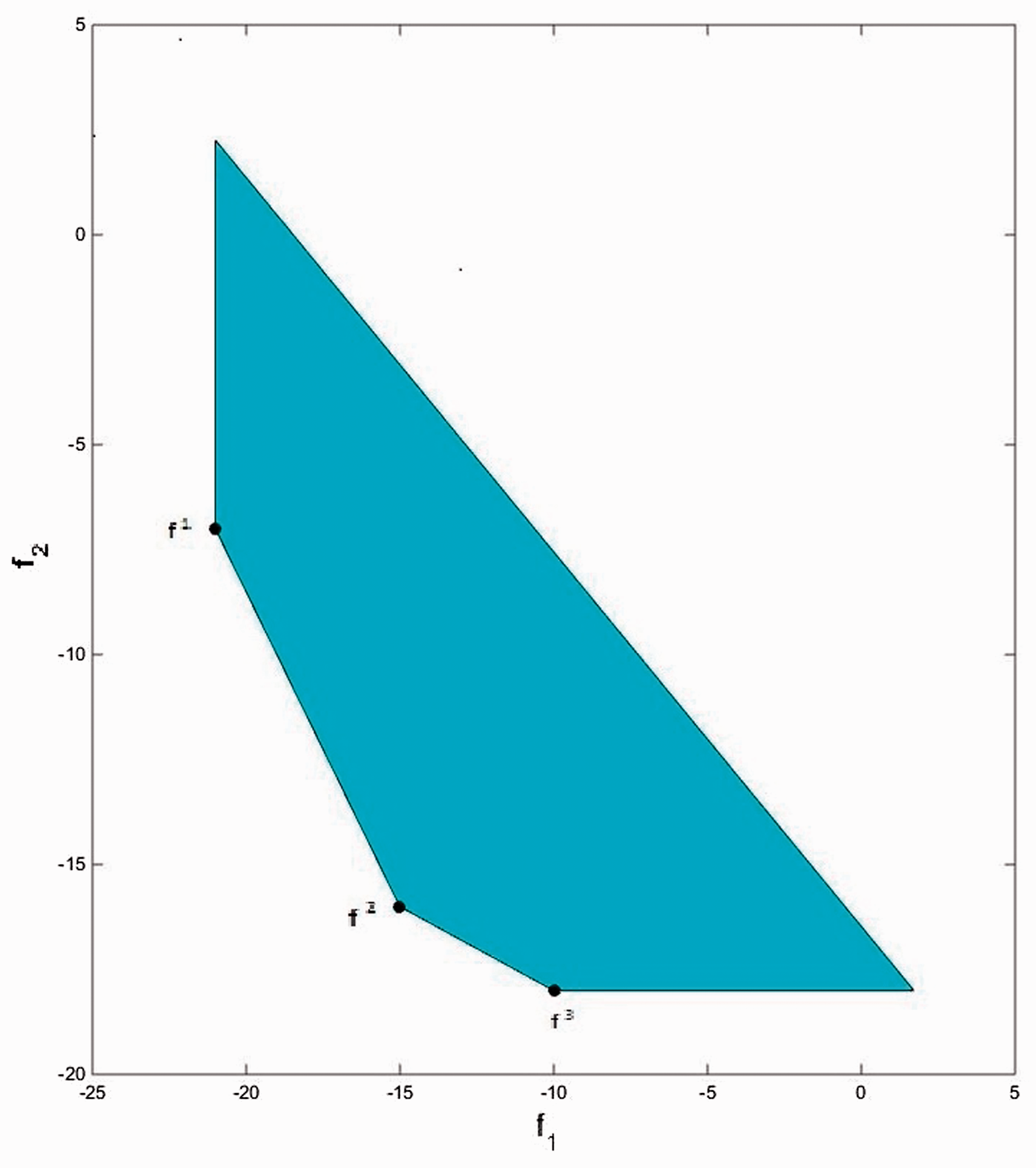
Nondominated edges connecting the three points in the objective space.

Selection of the MPNP

This issue has been alluded to in the introduction. To determine the MPNP, we employ the technique of Compromise Programming (CP) introduced by Zeleny ²⁵ and compute the ideal objective point which would serve as a reference point in each case. CP is a mathematical programming method that is based on the notion of distance of a most preferred solution from the ideal point $y^{*}$ . ²⁶ CP can be used to find the best nondominated point by determining the minimum distance to the ideal point. ²⁷ Ehrgott and Tenfelde-Podehl ²⁸ note that the ideal point is an essential component of CP, and the idea is to find a nondominated point which is as close as possible to it. This is a point in the objective space whose components are the optimal values of the objective functions when they are individually optimized. ²⁴ It was also noted in Zeleny ²⁶ that the ideal point serves as a rationale directing and facilitating human choice and decision making. To find the ideal point, we simply solve q single objective problems

$$\begin{array}{c}\text{min}{c}_k^{T}x,k=1,2,\dots ,q\\ \text{subject to}x\in X\end{array}$$

(4)

We note here that the ideal point itself is not an element of the nondominated set $(y^{*}\notin Y_N)$ . Otherwise, this would mean that the objective functions are not conflicting, but it always exists in the objective space. Its corresponding point in the decision space may not exist. ²⁴

For our numerical illustration above (Problem 3 of ‘Illustration of PSA’ section), solving each of the objective functions individually over the feasible region X yields the ideal objective point $y^{*}={(-21.0,-18.0)}^T$ . Clearly, $y^{*}\notin Y_N$ , where $Y_N=\{{(-10.0,-18.0)}^T,{(-15.0,-16.0)}^T,{(-21.0,-7.0)}^T\}$ as returned by PSA and BOA for this problem.

Having computed the ideal objective point $y^{*}$ , we now determine the minimum distance of each nondominated point $\widehat{y}$ from it by finding

$$\text{min}\{\Vert {\widehat{y}}_1-y^{*}\Vert ,\Vert {\widehat{y}}_2-y^{*}\Vert ,\dots ,\Vert {\widehat{y}}_n-y^{*}\Vert \}$$

where ${\widehat{y}}_i\in Y_N$ has already been found either by PSA or BOA, $\Vert .\Vert$ is the Euclidean norm on ${\mathbb{ℝ}}^q$ and $y^{*}$ is the ideal objective point. Using the nondominated points f¹, f² and f³ for Problem 3 yield

$$\begin{array}{c}\Vert f^1-y^{*}\Vert =11.0,\Vert f^2-y^{*}\Vert =6.3\\ \text{ and }\Vert f^3-y^{*}\Vert =11.0\end{array}$$

Since the relative distance of f² from the ideal point $y^{*}$ is 6.3 which is the smallest of the three, it therefore means that $f^2={(-15.0,-16.0)}^T$ is the closest of the three nondominated points to the ideal point $y^{*}={(-21.0,-18.0)}^T$ . Hence, f² is selected as the DM’s MPNP.

The following more substantial illustrative MOLP adapted from Zeleny ⁹ with three objectives makes the point

$$\begin{array}{l}\text{min}{f}_1=-x_1-2x_2+x_3-3x_4-2x_5-x_7\\ \text{min}{f}_2=-x_2-x_3-2x_4-3x_5-x_6\\ \text{min}{f}_3=-x_1-x_3+x_4+x_6+x_7\\ \text{Subject}\text{to}\\ x_1+2x_2+x_3+x_4+2x_5+x_6+2x_7\le 16\\ -2x_1-x_2+x_4+2x_5+x_7\le 16\\ -x_1+x_3+2x_5-2x_7\le 16\\ x_2+2x_3-x_4+x_5-2x_6-x_7\le 16\\ x_1,x_2,x_3,x_4,x_5,x_6,x_7\ge 0\end{array}$$

(5)

Again, optimizing each of the objective functions individually over the feasible region yields the ideal objective point $y^{*}={(-48.0,-32.0,-16.0)}^T$ . Solving Problem 5 with BOA, the set of nondominated points found is $Y_N=\{{(-48.0,-32.0,16.0)}^T,{(-16.0,0.0,-16.0)}^T,{(0.0,-8.0,-16.0)}^T,{(-5.33,-21.33,-5.33)}^T,{(-16.0,-24.0,0.0)}^T\}$ with $y^{*}\notin Y_N$ . By determining the minimum distance of each of these nondominated points from the ideal point $y^{*}$ , it was found that the point ${(-48.0,-32.0,16.0)}^T$ is the closest. Its distance from it is 32. It is selected as the DM’s MPNP.

For PSA, the set of nondominated points found is $Y_N=\{{(-8.0,-4.0,12.0)}^T,{(-16.0,0.0,-16.0)}^T,{(0.0,-8.0,8.0)}^T,{(-8.0,0.0,8.0)}^T\}$ also with $y^{*}\notin Y_N$ .

Next, we measure the distances of each of these points from the ideal point $y^{*}={(-48.0,-32.0,-16.0)}^T$ as was done with those returned by BOA. It turned out that the nondominated point ${(-16.0,0.0,-16.0)}^T$ is the closest to the ideal point $y^{*}$ and is selected as the DM’s MPNP as shown in Table 1, Problem 9. Its distance from it is 55.42 which is bigger than 32 which was the closest when measuring the points returned by BOA, thereby making the MPNP returned by BOA closer to the ideal point and of higher quality for this problem.

Table 1.

Summary of experimental results.

	Criteria for evaluation
Algorithms	Computing efficiency		Robustness	Quality of MPNP
	Degenerate problems	Non-degenerate problems
BOA	Computationally superior to PSA on highly degenerate problems	Computationally inferior to PSA on non-degenerate problems	Outperforms PSA in terms of robustness of methods	Returned high quality MPNP than PSA on highly degenerate problems
PSA	Computationally inferior to BOA on highly degenerate problems	Computationally more efficient than BOA on non-degenerate problems	Not so robust as compared to BOA	Returned high quality MPNP as BOA for most of the problems considered

We have used this method to choose the MPNP from the nondominated sets returned by PSA and BOA for comparison. The measure of the quality of solutions used is the distance to the ideal point as explained above.

Experimental results

In this section, we provide numerical results to compare the computing efficiency, robustness and the quality of a MPNP returned by Algorithms 1 and 2.

Table 2 shows the numerical results for a collection of 53 problems, from the existing literature. Problem 1 is taken from Ehrgott, ¹ Problems 2–10 were taken from Zeleny. ²⁶ Problems 11–21 are test problems from the interactive MOLP explorer (iMOLPe) of Alves et al. ²⁴ Problems 22–47 are taken from Steuer. ¹² Problems 48 and 53 are test problem in Bensolve-2.0 of Löhne and Weißing, ²⁹ while Problem 52 is a test problem in Bensolve-1.2 of Löhne. ²⁰ Finally, Problems 49–51 are obtained using a script in Bensolve-2.0 of Löhne and Weißing ²⁹ that was used to generate problem 53 with the same number of variables and constraints. Problem 48 has a dense constraint matrix with an identity matrix of order n as its criterion matrix, where n is the number of variables in the problem. The RHS vector is such that all the components are zeros except for a one (1) at the beginning as the only none zero element. Problems 49–51 and 53 have dense criterion matrices with identity matrices of order n as their constraint matrices, where n is also the number of variables in the respective problem. All the elements in the RHS vectors are ones. Finally, Problem 52 is such that the constraint matrix is sparse while the criterion matrix is dense. The RHS vector is such that all the components are ones except for 200 at the end as the largest entry.

Table 2.

Comparative results for small to medium instances.

Algorithms					BOA			PSA
Prob.	Origin	n	m	q	NNP	MPNP	CPU (s)	NNP	MPNP	CPU (s)
1	Ehrgott 1	3	3	3	3	f1 = –2.00	0.038	3	f1 = –2.00	0.031
						f2 = 10.00			f2 = 10.00
						f3 = –5.00			f3 = –5.00
2	Zeleny26	2	2	2	3	f1 = –25,000	0.021	3	f1 = –25,000	0.015
						f2 = –66,667			f2 = –66,667
3	Zeleny 26	2	4	2	2	f1 = –9.00	0.026	2	f1 = –9.00	0.019
						f2 = –15.00			f2 = –15.00
4	Zeleny 26	2	4	3	3	f1 = –3.00	0.161	3	f1 = –3.00	0.121
						f2 = –7.50			f2 = –7.50
						f3 = 9.00			f3 = 9.00
5	Zeleny 26	2	6	2	3	f1 = –24.00	0.212	3	f1 = –24.00	0.181
						f2 = –16.00			f2 = –16.00
6	Zeleny 26	3	3	3	5	f1 = 3.00	0.046	5	f1 = 3.00	0.032
						f2 = –6.00			f2 = –6.00
						f3 = –12.00			f3 = –12.00
7	Zeleny 26	5	3	3	4	f1 = 0.00	0.043	4	f1 = 0.00	0.041
						f2 = –4.00			f2 = –4.00
						f3 = –24.00			f3 = –23.62
8	Zeleny 26	5	2	2	1	f1 = –52.00	0.016	1	f1 = –52.00	0.011
						f2 = –52.00			f2 = –52.00
9	Zeleny 26	6	4	2	1	f1 = 0.00	0.017	1	f1 = 0.00	0.012
						f2 = 0.00			f2 = 0.00
10	Zeleny 26	7	4	3	5	f1 = –48.00	0.163	4	f1 = –16.00	0.152
						f2 = –32.00			f2 = 0.00
						f3 = 16.00			f3 = –16.00
11	iMOLPe	2	3	2	3	f1 = –21.00	0.047	3	f1 = –21.00	0.035
						f2 = –7.00			f2 = –7.00
12	iMOLPe	3	3	4	3	f1 = –10.00	0.033	3	f1 = –10.00	0.021
						f2 = –20.00			f2 = –20.00
						f3 = –100.00			f3 = –100.00
						f4 = –10.00			f4 = –10.00
13	iMOLPe	3	5	3	10	f1 = –21.00	0.042	10	f1 = –21.00	0.033
						f2 = –4.50			f2 = –4.50
						f3 = –4.00			f3 = –4.00
14	iMOLPe	3	3	3	7	f1 = –2.66	0.035	7	f1 = –2.66	0.032
						f2 = –2.00			f2 = –2.00
						f3 = –0.33			f3 = –0.33
15	iMOLPe	4	3	3	8	f1 = –48.50	0.038	8	f1 = –48.50	0.036
						f2 = –19.50			f2 = –19.50
						f3 = –37.00			f3 = –37.00
16	iMOLPe	4	2	3	6	f1 = –20.00	0.036	6	f1 = –20.00	0.035
						f2 = –80.00			f2 = –80.00
						f3 = –40.00			f3 = –40.00
17	iMOLPe	4	4	3	11	f1 = –40.00	0.186	11	f1 = –40.00	0.162
						f2 = –50.00			f2 = –50.00
						f3 = –10.00			f3 = –10.00
18	iMOLPe	3	3	3	5	f1 = 0.00	0.033	5	f1 = 0.00	0.031
						f2 = –2.00			f2 = –2.00
						f3 = –4.00			f3 = –4.00
19	iMOLPe	15	10	2	11	f1 = –363.82	0.195	7	f1 = –229.18	0.125
						f2 = –33.70			f2 = –35.31
20	iMOLPe	15	10	3	37	f1 = –363.82	0.476	7	f1 = –134.17	0.301
						f2 = –33.70			f2 = –32.88
						f3 = –136.71			f3 = –135.82
21	iMOLPe	10	5	3	14	f1 = 226.40	0.623	14	f1 = 223.09	0.589
						f2 = –501.86			f2 = –496.23
						f3 = –351.14			f3 = –246.64
22	Steuer 12	5	5	2	5	f1 = –10.00	0.036	5	f1 = –10.00	0.034
						f2 = –3.00			f2 = –3.00
23	Steuer 12	4	4	3	3	f1 = 3.42	0.015	3	f1 = 3.42	0.012
						f2 = –10.28			f2 = –10.28
						f3 = –3.42			f3 = –3.42
24	Steuer 12	5	5	4	14	f1 = 1.02	0.098	14	f1 = 1.02	0.081
						f2 = –25.46			f2 = –25.46
						f3 = 24.44			f3 = 24.44
						f4 = –28.32			f4 = –28.32
25	Steuer 12	10	8	4	72	f1 = 106.29	1.973	65	f1 = 183.36	0.921
						f2 = –462.13			f2 = –424.26
						f3 = 175.57			f3 = 117.29
						f4 = –33.41			f4 = –4.03
26	Steuer 12	5	4	3	9	f1 = –52.07	0.054	8	f1 = –52.07	0.045
						f2 = 31.50			f2 = 31.50
						f3 = –17.35			f3 = –17.35
27	Steuer 12	6	8	4	14	f1 = –6.94	0.065	6	f1 = –6.94	0.053
						f2 = –5.38			f2 = –5.38
						f3 = 6.83			f3 = 6.83
						f4 = –9.16			f4 = –9.16
28	Steuer 12	7	6	4	15	f1 = –31.53	0.286	12	f1 = –31.53	0.555
						f2 = –26.48			f2 = –26.48
						f3 = –26.57			f3 = –26.57
						f4 = –0.34			f4 = –0.34
29	Steuer 12	7	6	4	9	f1 = 26.80	0.192	9	f1 = 26.80	0.142
						f2 = –37.73			f2 = –37.73
						f3 = –24.33			f3 = –24.33
						f4 = –59.60			f4 = –59.60
30	Steuer 12	8	8	6	286	f1 = –74.00	73.963	40	f1 = –77.00	0.699
						f2 = –107.50			f2 = –52.00
						f3 = –41.25			f3 = –16.00
						f4 = –27.25			f4 = –52.40
						f5 = –9.00			f5 = 26.00
						f6 = –30.75			f6 = –20.00
31	Steuer 12	8	8	3	5	f1 = –36.57	0.168	5	f1 = –36.57	0.156
						f2 = –22.28			f2 = –22.28
						f3 = –14.00			f3 = –14.00
32	Steuer 12	8	8	3	12	f1 = –14.03	0.135	1	f1 = –6.50	0.121
						f2 = –18.00			f2 = –11.00
						f3 = –4.93			f3 = –7.50
33	Steuer 12	5	5	4	12	f1 = –21.50	0.277	8	f1 = –8.00	0.216
						f2 = –39.25			f2 = –23.87
						f3 = –16.25			f3 = –7.62
						f4 = 27.00			f4 = 27.00
34	Steuer 12	6	6	3	17	f1 = –12.65	0.212	17	f1 = 13.62	0.210
						f2 = 0.00			f2 = –9.75
						f3 = –30.15			f3 = –26.25
35	Steuer 12	5	5	4	9	f1 = –14.66	0.462	2	f1 = –14.00	0.345
						f2 = –21.06			f2 = 0.00
						f3 = 35.73			f3 = 27.00
						f4 = –16.00			f4 = 0.00
36	Steuer 12	10	10	4	6	f1 = 46.50	0.333	6	f1 = 46.50	0.241
						f2 = 19.21			f2 = 19.21
						f3 = –27.07			f3 = –27.07
						f4 = –27.07			f4 = –27.07
37	Steuer 12	8	8	3	13	f1 = –14.48	0.217	13	f1 = –14.48	0.201
						f2 = –4.74			f2 = –4.74
						f3 = 6.93			f3 = 6.93
38	Steuer 12	6	7	4	21	f1 = –2.61	0.386	a	–	–
						f2 = –12.63
						f3 = 9.70
						f4 = 2.37
39	Steuer 12	12	16	4	601	f1 = –5.25	31.034	23	f1 = –5.13	0.982
						f2 = –14.25			f2 = –3.38
						f3 = –8.25			f3 = 1.83
						f4 = –1.00			f4 = –1.18
40	Steuer 12	10	14	5	132	f1 = –5.16	102.952	9	f1 = –18.00	1.395
						f2 = –2.79			f2 = 70.60
						f3 = –4.38			f3 = –3.20
						f4 = –18.70			f4 = 8.00
						f5 = –9.69			f5 = –4.30
41	Steuer 12	7	6	3	3	f1 = –29.40	0.165	3	f1 = –29.40	0.151
						f2 = –65.30			f2 = –65.30
						f3 = –39.30			f3 = –39.30
42	Steuer 12	7	7	3	7	f1 = –62.18	0.036	7	f1 = –62.18	0.036
						f2 = –93.50			f2 = –93.50
						f3 = –52.00			f3 = –52.00
43	Steuer 12	6	6	4	5	f1 = –37.50	0.158	5	f1 = –37.50	0.134
						f2 = –11.25			f2 = –11.25
						f3 = –7.50			f3 = –7.50
						f4 = –20.25			f4 = –20.25
44	Steuer 12	6	6	4	10	f1 = 34.50	0.211	10	f1 = 34.50	0.201
						f2 = –7.50			f2 = –7.50
						f3 = –56.00			f3 = –56.00
						f4 = –31.50			f4 = –31.50
45	Steuer 12	10	14	5	471	f1 = 1.03	307.611	a	–	–
						f2 = –2.19
						f3 = 2.01
						f4 = –8.13
						f5 = 7.22
46	Steuer 12	10	14	5	128	f1 = –4.95	105.344	1	f1 = 4.93	0.291
						f2 = –3.42			f2 = –5.57
						f3 = –4.38			f3 = –2.83
						f4 = –18.91			f4 = –16.28
						f5 = –9.27			f5 = –6.13
47	Steuer 12	7	7	3	6	f1 = –3.83	0.045	9	f1 = –3.83	0.031
						f2 = –76.46			f2 = –76.46
						f3 = –49.57			f3 = –49.57
48	Bensolve-2.0	5	31	5	22	f1 = 0.00	2.877	1	f1 = 0.00	0.125
						f2 = –1.00			f2 = 0.00
						f3 = 0.00			f3 = 0.00
						f4 = 0.00			f4 = 0.00
						f5 = –2.00			f5 = 0.00
49	Bensolve-2.0	36	36	2	8	f1 = –5.00	0.211	82	f1 = –5.00	0.772
						f2 = –26.00			f2 = –25.50
50	Bensolve-2.0	64	64	2	14	f1 = –63.00	0.403	292	f1 = –34.50	5.167
						f2 = –7.00			f2 = –9.50
51	Bensolve-2.0	100	100	2	20	f1 = –124.00	0.621	1102	f1 = –123.50	36.323
						f2 = –9.00			f2 = –9.00
52	Bensolve-1.2	100	101	2	32	f1 = –8.42	0.503	a	–	–
						f2 = –116.65
53	Bensolve-2.0	343	343	3	1368	f1 = –42.00	55.302	b	–	–
						f2 = –294.00
						f3 = –6.00

^aThe image is the whole region, implying that the problem has no solution.

^bOut of memory.

Both Algorithms 1 and 2 were implemented in Matlab. In all tests, m is the number of constraints, n the number of variables, q the number of objectives and NNP the number of nondominated points returned by the algorithms. All problems were executed on an Intel Core i5-2500 CPU at 3.30 GHz with 16.0GB RAM. We recorded the CPU times (in seconds) returned by the algorithms for each problem and also acted as the DM by choosing a MPNP (whose components are as close as possible to the ideal objective point as explained in ‘Selection of the most preferred nondominated point’ section) from the nondominated set $Y_N=\{\mathit{Cx}:x\in X_E\}$ returned by PSA to compare with a MPNP returned by BOA.

As can be seen in Table 2, the CPU times increase as the problem dimension increases. We can also infer from Tables 2 and 3 that the CPU times also depend to some extent on the total number of nondominated points returned by the algorithm for a given problem. That is to say, the more the number of nondominated points in a given problem, the more computational effort would be required to obtain them. We note here that most of the problems in Table 2 are non-degenerate. For these problems, PSA appears to have computational advantage over BOA, most especially for those problems with more nondominated points as it returns only a subset of them; see problems 20, 25, 30, 39, 40 and 46. We noticed that for those problems where both algorithms return the same number of nondominated points, there is a slight difference in CPU time which is in favour of PSA. We also observed that PSA returns more nondominated points for some of the problems than BOA; this is not supposed to happen as it is meant to return a subset of these points. Some of the nondominated points returned are repeated. In terms of the quality of a MPNP returned by these algorithms, we observed in Table 2 that both algorithms returned the same MPNP points for most of the problems considered. However, for a few of these problems where the MPNP are not the same, BOA returned higher quality MPNP than PSA as illustrated in pages 15 and 16 (second numerical illustration of Problem 5). This observation may be largely due to the fact that PSA is not meant to return all nondominated points, as it returns a subset of them, whereas BOA returns all the nondominated points of the problem.

Table 3.

Comparative results for large instances (NNP stands for Number of Nondominated Points).

Algorithms					BOA			PSA
Prob.	Origin	n	m	q	NNP	MPNP	CPU (s)	NNP	MPNP	CPU (s)
54	Inner	844	12	10	1	f1 = –1.00, f2 = –1.00, f3= 0.00	0.871	1	f1 = 0.00, f2 = 0.00, f3= 0.00	2.835
						f4 = 0.00, f5 = 0.00, f6 = 0.00			f4 = 0.00, f5 = 0.00, f6 = 0.00
						f7 = 0.00, f8 = 0.00, f9 = 0.00			f7 = 0.00, f8 = 0.00, f9 = 0.00
						f10 = 0.00			f10 = 0.00
55	Inner	853	12	10	1	f1 = –1.00, f2 = –1.00, f3= 0.00	0.892	1	f1 = 0.00, f2 = 0.00, f3= 0.00	2.888
						f4 = 0.00, f5 = 0.00, f6 = 0.00			f4 = 0.00, f5 = 0.00, f6 = 0.00
						f7 = 0.00, f8 = 0.00, f9 = 0.00			f7 = 0.00, f8 = 0.00, f9 = 0.00
						f10 = 0.00			f10 = 0.00
56	Inner	857	12	10	1	f1 = –1.00, f2 = –1.00, f3= 0.00	0.871	1	f1 = 0.00, f2 = 0.00, f3= 0.00	2.922
						f4 = 0.00, f5 = 0.00, f6 = 0.00			f4 = 0.00, f5 = 0.00, f6 = 0.00
						f7 = 0.00, f8 = 0.00, f9 = 0.00			f7 = 0.00, f8 = 0.00, f9 = 0.00
						f10 = 0.00			f10 = 0.00
57	Inner	873	12	10	1	f1 = 0.00, f2 = –1.00, f3= –1.00	0.884	1	f1 = 0.00, f2 = 0.00, f3= 0.00	3.041
						f4 = 0.00, f5 = 0.00, f6 = 0.00			f4 = 0.00, f5 = 0.00, f6 = 0.00
						f7 = 0.00, f8 = 0.00, f9 = 0.00			f7 = 0.00, f8 = 0.00, f9 = 0.00
						f10 = 0.00			f10 = 0.00
58	Inner	877	12	10	1	f1 = 0.00, f2 = –1.00, f3= –1.00	0.935	1	f1 = 0.00, f2 = 0.00, f3= 0.00	3.071
						f4 = 0.00, f5 = 0.00, f6 = 0.00			f4 = 0.00, f5 = 0.00, f6 = 0.00
						f7 = 0.00, f8 = 0.00, f9 = 0.00			f7 = 0.00, f8 = 0.00, f9 = 0.00
						f10 = 0.00			f10 = 0.00
59	Inner	880	12	10	1	f1 = 0.00, f2 = –1.00, f3= –1.00	0.968	1	f1 = 0.00, f2 = 0.00, f3= 0.00	3.113
						f4 = 0.00, f5 = 0.00, f6 = 0.00			f4 = 0.00, f5 = 0.00, f6 = 0.00
						f7 = 0.00, f8 = 0.00, f9 = 0.00			f7 = 0.00, f8 = 0.00, f9 = 0.00
						f10 = 0.00			f10 = 0.00
60	Inner	882	12	10	1	f1 = –1.00, f2 = 0.00, f3= –1.00	1.009	1	f1 = 0.00, f2 = 0.00, f3= 0.00	3.115
						f4 = 0.00, f5 = 0.00, f6 = 0.00			f4 = 0.00, f5 = 0.00, f6 = 0.00
						f7 = 0.00, f8 = 0.00, f9 = 0.00			f7 = 0.00, f8 = 0.00, f9 = 0.00
						f10 = 0.00			f10 = 0.00
61	Inner	886	12	10	2	f1 = 0.00, f2 = 0.00, f3= 0.00	1.341	1	f1 = 0.00, f2 = 0.00, f3= 0.00	3.118
						f4 = 1.00, f5 = –1.00, f6 = –1.00			f4 = 0.00, f5 = 0.00, f6 = 0.00
						f7 = 0.00, f8 = 0.00, f9 = 0.00			f7 = 0.00, f8 = 0.00, f9 = 0.00
						f10 = 0.00			f10 = 0.00
62	Inner	888	12	10	1	f1 = –1.00, f2 = –1.00, f3= 0.00	1.104	1	f1 = 0.00, f2 = 0.00, f3= 0.00	3.119
						f4 = 0.00, f5 = 0.00, f6 = 0.00			f4 = 0.00, f5 = 0.00, f6 = 0.00
						f7 = 0.00, f8 = 0.00, f9 = 0.00			f7 = 0.00, f8 = 0.00, f9 = 0.00
						f10 = 0.00			f10 = 0.00
63	Inner	1009	12	10	1	f1 = 0.00, f2 = –1.00, f3= –1.00	1.281	1	f1 = 0.00, f2 = 0.00, f3= 0.00	3.911
						f4 = 0.00, f5 = 0.00, f6 = 0.00			f4 = 0.00, f5 = 0.00, f6 = 0.00
						f7 = 0.00, f8 = 0.00, f9 = 0.00			f7 = 0.00, f8 = 0.00, f9 = 0.00
						f10 = 0.00			f10 = 0.00
64	Inner	1956	12	10	1	f1 = –1.00, f2 = –1.00, f3= 0.00	4.288	1	f1 = 0.00, f2 = 0.00, f3= 0.00	13.374
						f4 = 0.00, f5 = 0.00, f6 = 0.00			f4 = 0.00, f5 = 0.00, f6 = 0.00
						f7 = 0.00, f8 = 0.00, f9 = 0.00			f7 = 0.00, f8 = 0.00, f9 = 0.00
						f10 = 0.00			f10 = 0.00
65	Inner	1983	12	10	1	f1 = 0.00, f2 = 0.00, f3= 0.00	4.418	1	f1 = 0.00, f2 = 0.00, f3= 0.00	13.805
						f4 = –1.00, f5 = –1.00, f6 = 0.00			f4 = 0.00, f5 = 0.00, f6 = 0.00
						f7 = 0.00, f8 = 0.00, f9 = 0.00			f7 = 0.00, f8 = 0.00, f9 = 0.00
						f10 = 0.00			f10 = 0.00
66	Inner	3722	338	10	55	f1 = –0.25, f2 = –0.50, f3= –2.75,	22.167	1	f1 = 0.00, f2 = 0.00, f3= 0.00	56.198
						f4 = 1.87, f5 = –0.62, f6 = 0.00,			f4 = 0.00, f5 = 0.00, f6 = 0.00
						f7 = 0.00, f8 = 0.00, f9 = 0.00			f7 = 0.00, f8 = 0.00, f9 = 0.00
						f10 = 0.00			f10 = 0.00
67	Inner	3725	338	10	61	f1 = –0.20, f2 = –0.40, f3= –2.40	24.605	1	f1 = 0.00, f2 = 0.00, f3= 0.00	56.458
						f4 = –2.20, f5 = –0.6, f6 = –0.20			f4 = 0.00, f5 = 0.00, f6 = 0.00
						f7 = 0.00, f8 = 0.00, f9 = 0.00			f7 = 0.00, f8 = 0.00, f9 = 0.00
						f10 = 0.00			f10 = 0.00
68	Inner	3897	362	10	b	–	–	a	–	–
69	Inner	5646	492	10	1575	f1 = –0.38, f2 = 0.00, f3= –2.55	125.488	1	f1 = 0.00, f2 = 0.00, f3= 0.00	130.159
						f4 = –1.66, f5 = –0.16, f6=–0.44			f4 = 0.00, f5 = 0.00, f6 = 0.00
						f7 = 0.00, f8 = 0.00, f9 = 0.00			f7 = 0.00, f8 = 0.00, f9 = 0.00
						f10 = 0.00			f10 = 0.00
70	Inner	8891	707	10	13	f1 = –0.20, f2 = 0.00, f3= –2.20,	228.312	1	f1 = 0.00, f2 = 0.00, f3= 0.00	329.701
						f4 = –2.20, f5 = –0.20, f6=–0.20			f4 = 0.00, f5 = 0.00, f6 = 0.00
						f7 = 0.00, f8 = 0.00, f9 = 0.00			f7 = 0.00, f8 = 0.00, f9 = 0.00
						f10 = 0.00			f10 = 0.00
71	Inner	9472	707	10	b	–	–	1	f1 = 0.00, f2 = 0.00, f3= 0.00	362.449
									f4 = 0.00, f5 = 0.00, f6 = 0.00
									f7 = 0.00, f8 = 0.00, f9 = 0.00
									f10 = 0.00
72	Inner	10017	779	10	31	f1=–0.11, f2 = 0.00, f3= –2.44	260.494	1	f1 = 0.00, f2 = 0.00, f3= 0.00	412.929
						f4 = –2.44, f5 = –0.55, f6=–0.55			f4 = 0.00, f5 = 0.00, f6 = 0.00
						f7 = 0.00, f8 = 0.00, f9 = 0.00			f7 = 0.00, f8 = 0.00, f9 = 0.00
						f10 = 0.00			f10 = 0.00
73	MOPLIB	30	21	12	1	f1=5.0E–12, f2=5.0E–12	0.598	1	f1 = 0, f2 = 0	0.167
						f3=5.0E–12, f4=5.0E–12			f3 = 0, f4 = 0
						f5=5.0E–12, f6=5.0E–12			f5 = 0, f6 = 0
						f7=5.0E–12, f8=5.0E–12			f7 = 0, f8 = 0
						f9=5.0E–12, f10=5.0E–12			f9 = 0, f10 = 0
						f11=5.0E–12, f12=–5.5E–11			f11 = 0, f12 = 0
74	MOPLIB	100	20	3	291	f1 = –168.00	4.291	1	f1 = –168.00	0.122
						f2 = –124.00			f2 = –124.00
						f3 = –143.00			f3 = –143.00
75	MOPLIB	53	221	3	2552	f1 = 0.00	1663.803	1	f1 = 0.00	0.682
						f2 = –2.00			f2 = 0.00
						f3 = –13959.00			f3 = –13461.00
76	MOPLIB	53	226	3	552	f1 = –180.00	6.551	74	f1 = –144.00	1.628
						f2 = –123.00			f2 = –79.00
						f3 = 16842.00			f3 = 13360.00
77	MOPLIB	1143	1211	3	c	–	–	1	f1 = –85.00, f2 = 0, f3 = 0	16.248
78	MOPLIB	36939	4608	3	c	–	–	1	f1 = 0, f2 = 0, f3 = 0	18927.102
79	MOPLIB	900	60	4	b	–	–	1	f1 = –434.00, f2 = –452.00	3.005
									f3 = –497.00, f4 = –463.00
80	MOPLIB	729	729	4	b	–	–	c	–	–
81	MOPLIB	4492	1003	4	c	–	–	1	–	–
82	MOPLIB	900	60	10	c	–	–	1	f1 = –394.00, f2 = –429.00	4.306
									f3 = –415.00, f4 = –428.00
									f5 = –447.00, f6 =–417.00
									f7 = –401.00, f8 = –414.00
									f9 = –402.00, f10 = –429.00
83	MOPLIB	779	10174	10	b	–	–	1	f1 = 0.00, f2 = 0.00	424.58
									f3 = 0.00, f4 = 0.00
									f5 = 0.00, f6 = 0.00
									f7 = 0.00, f8 = 0.00
									f9 = 0.00, f10 = 0.00
84	MOPLIB	376	1917	19	c	–	–	1	f1 = 2, f2 = –1, f3 = –1	69.765
									f4 = –1, f5 = 0, f6= –1,
									f7 = 0, f8 = –1, f9= 0,
									f10 = –1, f11 = –2, f12= –2
									f13 = 0, f14 =0, f15 = 0
									f16 = 0, f17 = 0, f18 = 0,
									f19 = 0.
85	MOPLIB	218	28	27	b	–	–	1	f1 = –360, f2 = 0, f3 = 0	14.746–
									f4 = 90, f5 = 180, f6 = 180
									f7 = 180, f8 = 180, f9 = 270
									f10 = 0, f11 = 360, f12 = 90
									f13 = 180, f14 = 0, f15 = 90
									f16 = 90, f17 = 0, f18 = –90,
									f19 =  90, f20 = –90, f21 = –90
									f22 = 90, f23 = –90, f24 = –90
									f25 = –90, f26 = 90, f27 = 0.
86	MOPLIB	295056	24586	2	c		–	c	–

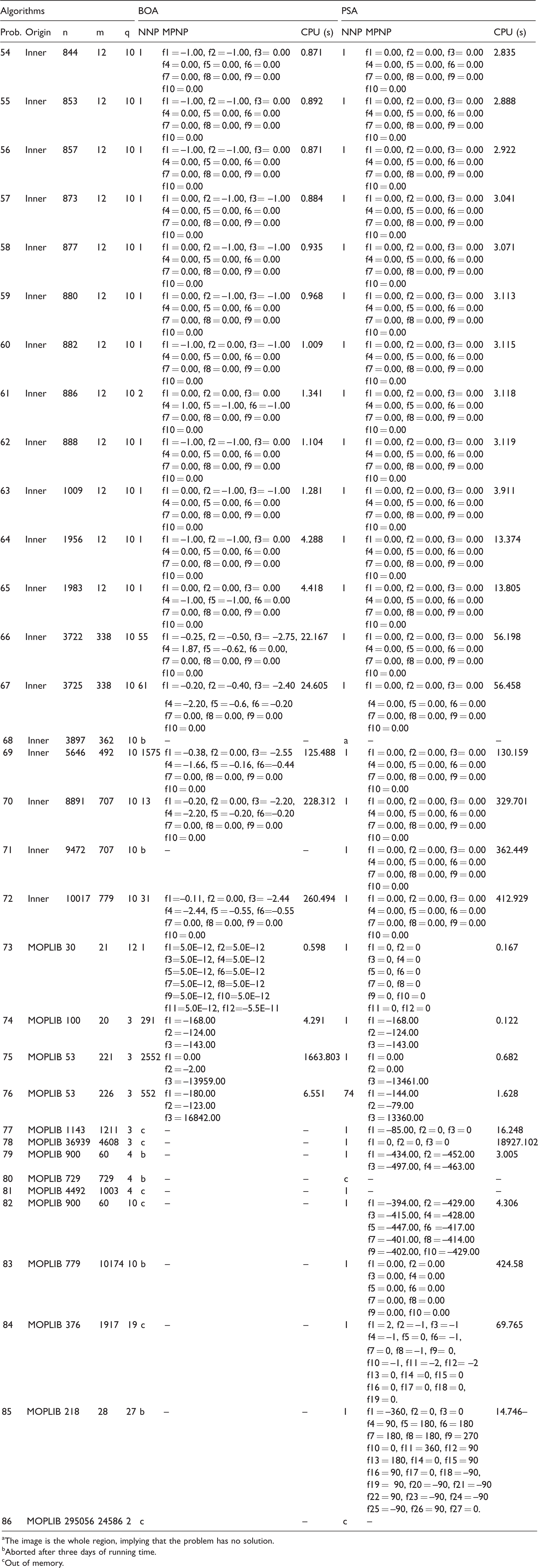
^aThe image is the whole region, implying that the problem has no solution.

^bAborted after three days of running time.

^cOut of memory.

Next, we use practical size MOLP instances from Csirmaz ³⁰ which is an MOLP solver called Inner and MOPLIB³¹ which stands for Multi-Objective Problem Library. These test problems were also executed on the same machine, and the results are reported in Table 3.

Problems 54–72 are from Csirmaz ³⁰ while Problems 73–86 are from MOPLIB. Note that Problems 54–73 are highly degenerate. Their structure is such that their constraint and criterion matrices are sparse while all the components of the RHS vectors are zeros except for a one (1) as the only non-zero entry. In Problems 74 and 79, the constraint matrices are sparse, the criterion matrices are dense and all the elements in the RHS vectors are ones. Problems 75 and 76 have sparse constraints and criterion matrices with dense RHS vectors. Problem 78 is such that the RHS vector is dense while the constraint and criterion matrices are sparse. In Problems 80 and 82, the constraint matrices are sparse, criterion matrices are dense and all the elements in the RHS vectors are ones. Problems 77 and 81 have dense RHS vectors while the constraint and criterion matrices are sparse. Problems 83 and 84 are such that the constraint and criterion matrices are sparse, and all the components of the RHS vectors are zeros except for a one (1) at the beginning as the only non-zero element. Problem 85 is such that the constraint and criterion matrices are sparse while the components of the RHS vector are all zeros except for a 90 at the end as the only non-zero entry. Finally, Problem 86 is such that the constraint and criterion matrices as well as the RHS vector are all sparse. For the highly degenerate problems, it was observed that BOA is computationally superior to PSA which confirms what was reported by Rudloff et al. ³ that BOA outperforms PSA on highly degenerate problems. Even the nondominated points returned by PSA for these problems are also of lower quality than those returned by BOA.

In terms of robustness of methods, we noticed in Tables 2 and 3 that PSA could not solve problems 38, 45, 52, 68 and 81. It returns the image which is the whole region which indicates that none of the vertices in the image is nondominated, meaning that no solution is returned thereby making BOA more robust. However, we also observed in Table 3 that BOA could not produce results for some of the test problems despite the long running time allowed (three days); it was aborted. The fact that some problems were aborted after three days of running time does not necessarily mean that the algorithms cannot solve these problems; if allowed to run further, they could potentially return a huge number of nondominated points or run out of memory which would indicate that the total number of nondominated points has exceeded the Matlab storage capacity on the machine used.

For those problems which were solved by BOA in Table 3, it was also observed that the MPNPs returned are of higher quality than those returned by PSA. However, for the non-degenerate problems, PSA was found to be computationally superior to BOA.

Summary of results

In this section, we present the summary of experimental results discussed in the previous section in Table 1. We have also presented the CPU time of BOA and PSA for 70 out of the 86 instances (which represent 81.40%) of the total problems solved by both methods in Figure 3.

Figure 3.

Running time of PSA and BOA for the 70 instances solved.

Conclusion

We have reviewed the existing literature on the parametric simplex and Benson’s BOAs. We have also presented these algorithms, explained and illustrated them on small MOLP instance. Crucially, we have explained how MPNP’s are obtained. A detailed computational experience to compare the efficiency, robustness as well as the quality of MPNP’s is provided. The CPU times and quality of MPNP’s returned by these algorithms for a collection of 86 existing MOLP problems, ranging from small to medium and practical size instances is reported. It was observed that BOA is superior to PSA in terms of robustness, quality of the MPNP’s it returns and is also computationally more efficient than PSA on highly degenerate problems. The measure of quality used is the distance to the ideal point as explained in ‘Experimental results’ section. However, PSA outperforms BOA on non-degenerate problems.