Parallel multibody separation simulation using MPI and OpenMP with communication optimization

Abstract

In this paper we investigate parallel implementations of multibody separation simulation using a hybrid of message passing interface and OpenMP. We propose a mesh block-based overset communication optimization algorithm. After presenting details of local data structures, we present our strategy for parallelizing both the overset mesh assembler and the flow solver by employing message passing interface and OpenMP. Experimental results show that the mesh block-based overset communication optimization algorithm has an advantage in real elapsed time when compared to a process-based implementation. The hybrid version shows that it is suitable for improving the load balance if a large number of CPU cores are used. We report results for a standard multibody separation case.

Introduction

Simulations of multibody separation (MBS) are classified as moving body problems in the field of computational fluid dynamics (CFD). The overset mesh approach^1,2,5,9 is an effective mesh technique for MBS calculations. In this approach, an independent mesh system models each entity, and different mesh systems may overlap. Therefore, this technique makes handling relative motion between entities in MBS problems more straightforward. However, the overset mesh assembler (OMA), which determines and optimizes overlapping regions and arranges the interpolated information among overlapped mesh blocks, must be used for preprocessing prior to computing the steady flow. Plus, it must be performed for each physical time step if relative motions exist between two entities in the simulation of unsteady flow. Various OMAs, such as PEGASUS, ⁹ DCF3D, ¹⁰ SUGGAR/DiRTLib,^11,12 and C3LIB, ¹⁶ have been developed as overset mesh preprocessors.

The calculations that are associated with OMA and MBS problems have been widely reported. Barszcz et al. ¹³ used message passing interface (MPI) ²² to implement the parallel version of DCF3D and integrated it with OVERFLOW ²⁹ solver, and Wissink et al. ¹⁴ explored parallel performance with load balancing scheme for dynamic overset grid applications. Prewitt et al. ³ reviewed parallel implementations related to overset mesh methods and addressed the parallel approaches for the grid assembly function to prevent the grid assembly function from affecting the overall performances, but the number of processors used was limited to 50 cores and the parallel scale was relatively small. Pandya et al. ¹⁵ integrated the USM3D flow solver with the DiRTlib to study the dynamic overset case. Unfortunately, parallel aspects were not included in their work. Zagaris et al. ⁸ identified the primary challenges for MBS problems as arranging internal grid boundaries, detecting overlap regions and orphan points distributedly, and developing load balancing algorithms, and they presented techniques for parallel overset grid assembly and only reported the preliminary performance on a relatively small number of processors. Motivated by Zagaris’s work, Roget and Sitaraman ⁶ proposed and investigated large-scale parallel OMA and an adaptive load rebalancing algorithm on unstructured meshes, and the rebalancing algorithm had a great advantage in improving the parallel efficiency of unsteady calculations when nearly 10,000 cores are used. Landmann and Montagnac ⁷ proposed a parallel automated overset grid algorithm for complex configurations. It is shown in their work that the approach was well suited for steady flow simulations, but the unsteady flows or moving body simulations were not involved. Djomehri and Jin ²⁹ investigated the parallel performance of the OVERFLOW-D solver, which combines MPI ²² and OpenMP ²¹ , but they only presented steady results. Other flow simulations based on the overset mesh approach can be found in the literature.^4,17–20

However, the existing works focused either on singular parallel approach or on steady simulations by using overset method, and few works have addressed the hybrid parallel algorithms for unsteady problems of simulating MBS. As contemporary parallel systems consist of multicore nodes, an approach that uses a hybrid of MPI and OpenMP is very popular to make better use of multicore architectures. In this approach,^37–40 MPI level is considered for coarse parallelism and OpenMP level is considered for fine parallelism. Motivated by these studies, we propose a fully parallelized MPI+OpenMP implementation for MBS simulation and an investigation of a mesh block approach for data exchange in overlapping regions to improve the parallel scalability of the multiblock solver. Our main contributions are as follows.

We propose and implement a mesh block-based overset communication optimization (MBBOCO) algorithm, with a comparison of our strategy and process-based implementations on up to 1024 processor cores.

We develop a hybrid MPI+OpenMP approach for MBS simulation and present the implementation details of the OMA and core of the solver.

We perform an MBS simulation of a standard wing case to validate the accuracy and performance of the solver with 256 cores.

We have organized our paper as follows. We first introduce the overset mesh system and the unsteady procedure for MBS and propose our MBBOCO algorithm in the next section. In “Hybrid parallelization” section, we present our MPI+OpenMP implementation. In “Experiments” section, we report the performance of MBBOCO with up to 1024 CPU cores and the performance for our hybrid approach. The last section summarizes our work.

MBBOCO

Overset mesh system

We based the overset technique in the present paper on the multiblock structured overset mesh method. ² Multiblock mesh technique is still popular because it can provide convenience in implementing high-order spatial differencing and implicit time-stepping schemes due to its linear address space. It also can offer well-controlled fine grids at walls easily to resolve boundary layers accurately. Although it is not flexible in tackling complex geometries, the shortcoming can be made up for by combining the overset mesh approach. In the multiblock overset mesh technique, each geometric entity or component is configured by a multiblock structured mesh system consisting of many one-to-one mesh blocks. Only the mesh systems corresponding to different components may overlap with each other. Therefore, the moving parts are always modeled independently, without considering the mesh systems of static components, in the MBS calculations. This kind of overset mesh system differs from that in the popular OVERFLOW ³⁶ solver, as the latter employs a pure overset mesh system without a one-to-one mesh topology. Thus, data exchange should be taken care for both one-to-one mesh block pairs and overlapped mesh block pairs in parallel computing environment.

Unsteady procedure for MBS

Figure 1 provides a diagram of the unsteady process using multiblock mesh without moving or overlapping meshes and without considering the computations in the blue dashed boxes. The process consists of an outside physical time step loop and an inner pseudo-time cycle within each physical time cycle.

Figure 1.

Unsteady flowchart for MBS. MPI: message passing interface; NC: number of pseudo cycles; PC: pseudo-cycle; 6DOF: six degrees of freedom; UC: unsteady cycle.

As mentioned in the “Introduction” section, MBS simulations always require overset mesh techniques to handle moving parts of the given configuration. Before performing overset mesh computations in parallel, preprocessing is required to establish the interpolation information between each mesh block pair. There are three types of blocks in a multiblock mesh system, as illustrated by Figure 2. Interpolation-providing mesh blocks (IPMBs, such as block F in Figure 2) give interpolation information for one or more blocks. Interpolation-receiving mesh blocks (IRMBs, such as block E) receive interpolation information from IPMBs. Regular mesh blocks (RMBs, such as blocks A and B) do not overlap any other blocks. As Figure 2 shows, a single mesh block can be both IPMB and IRMB simultaneously, as is the case with blocks C and D.

Figure 2.

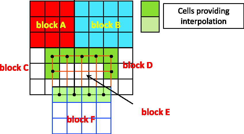
Mesh block types in overset grid system.

In view of Figure 1 and the three mesh types, we can perform unsteady computation via multiblock overset mesh in parallel by adding three additional steps (marked by blue dashed boxes in Figure 1):

Each IPMB sends interpolated flow quantities to the remote processes for dependent mesh blocks if the IPMB’s flow solution has been updated in the last time step.

Each IRMB on each process uses the data from IPMBs (local or remote) to update the flow solutions on overset boundaries before the one-to-one boundary data exchange in the next time step.

The system updates and reassembles meshes with six degrees of freedom (6DOF) between adjacent physical time steps.

Mesh block-based communication strategy

In this section, we present our block-based overset communication strategy and its implementation details.

During the parallel calculations on a distributed system, the solutions for blocks on a given computing node are updated one by one. As each solution is updated, interpolation data are sent to remote processes immediately using nonblocking MPI functions. And the communication overhead on an IPMB could be hidden by the flow computing of other mesh blocks on the same process. Algorithm 1 shows this communication algorithm.

Algorithm 1. Mesh block-based communication algorithm.

1: do iblock=1,Nblock

2:  if(PROCESS_ID.eq. BLOCK_TO_PROC(iblock)) then

3:    iblock: spatial discretization

4:    iblock: residual computation

5:    iblock: advancement in time

6:    iblock: update flow quantities

7:     MPI communication (lines 11–20)

8:  end if

9: end do

10:      // MPI communication —————

11: if(PROCESS_ID.eq. BLOCK_TO_PROC(iblock)) then

12:    //send the providing information of iblock to remote processes

13:    call MPI_ISend(dest_process: BLOCK_TO_PROC(relate_blocks))

14: else

15:    //iblock does not reside the process with PROCESS_ID,

16:    //receive the possible information from BLOCK_TO_PROC(iblock)

17:    if(blocks in this process need information from iblock) then

18:     call MPI_IRecv(source process:BLOCK_TO_PROC(iblock))

19:  end if

20: end if

As communication is per block and a single process usually manages more than one block, a sending–receiving process pair may communicate more than once. For example, if two different mesh blocks on process M (PM) send data to mesh blocks on remote process N (PN), repeated communication between PM and PN is inevitable. Also, a mesh block on PM may provide data for different blocks on the same remote process PN (where PM and PN are not the same), which would require PN to launch more than one MPI receiving operation to handle data incoming from PM. A message-packing technique avoids the latter case.

Figure 3 illustrates the one-way communication procedure where all mesh blocks on process M are IPMBs and all mesh blocks on process N are IRMBs. Block A provides data for all the four blocks on process N but it will pack data in the send buffer and communicate with PN only once when the block loop process (line 1–9) encounters iblock as block A. Likewise, IRMB blocks B, C, G, and H, which need the data from block A, will receive updates from process N in the same transmission. With this approach, the first communication between processes M and N occurs when the do loop encounters block A. Subsequent communication between processes M and N takes place when the solutions for blocks D, E, and F have been updated.

Figure 3.

Illustration of communication among overset mesh blocks.

Process-to-process (PTP) communication uses nonblocking MPI functions so that the overhead of transmitting data between IPMBs and IRMBs can be overlapped with mesh block flow calculations. Since there may be thousands of mesh blocks in a large-scale MBS simulation on more than 1024 CPU cores, we must choose optimal data structures and algorithms.

For efficient communication, we incorporate the following features.

S1: Each IPMB on a specified process allocates and manages two integer arrays.

One array denoted as S_blks stores all the identifiers of dependent blocks (i.e. those needing data from this IPMB) in ascending order.

The other array denoted as R_blks stores all the identifiers of blocks that provide data for this block (as an IRMB) in ascending order.

S1: Each IPMB on a specified process maintains a double-typed array S_buffer to store the data segments required by remote IRMBs in ascending order of the IRMB process identifier. If two different IRMBs have the same process identifier, the data segment associated with the smaller block identifier ranks ahead. This step guarantees that the data transmission from the same block to different processes is continuous.

S1: Each process merges all R_blks arrays into a new array sorted by block identifiers in ascending order and uses the new array to allocate R_buffer as the receiving buffer on each process.

Figure 4 shows how MPI communication takes place using these structures. Block B is the first IPMB visited during the block cycle on all processes, and process P2 provides two segments of data for remote blocks E and A, respectively. At the same time, process P3 containing block A has checked that it needs the interpolated data from P2 and initiates an MPI receiving operation to accept data. With the block cycle process in Algorithm 1, P3 conducts receiving operations one by one, filling the receive buffer from beginning to end without gaps or fragmentation. The numbers on the arrow lines give the sequence of sending and receiving operations in this example. However, the construction of our data structures requires the output of the OMA to distinguish IPMBs from IRMBS to count the number of sending and receiving points from them.

Figure 4.

Data structure, sending–receiving procedures for mesh block-based communication mode.

The proposed strategy provides several benefits. To begin with, it makes the communication of overset regions overlap with the computations, which can stop the extreme block with overloaded communication from affecting overall load balancing. Moreover, the design of data structure is purely local based, which avoids the use of global arrays and are of well data scalability. In addition, it is efficient because receiving buffers are designed to receive data sequentially and continuously without requirements of extra memory operations.

Hybrid parallelization

Hybrid parallelization for OMA

The OMA used here was developed especially for the overset mesh system described in “Overset mesh system” section. Similar to PEGASUS, ⁹ it requires the number of entities or components and the corresponding starting and ending mesh block identifier for each mesh system. Implemented in Fortran 90, it has the following features:

It combines hole mapping ³⁴ and inverse point searching to reduce the memory requirements of the auxiliary mesh.

It is cell center based and can search four (2D) or eight (3D) donor cells across processes.

It has two parallel versions, standalone and integrated. The stand-alone version requires the flow input as input. The integrated version is actually a subroutine that accepts necessary variables in the numerical solver as input parameters and writes the corresponding memory spaces (variables, arrays) allocated by the solver.

It uses the octree bounding box (OBB) technique ³⁵ to accelerate the parallel donor search and optimizes communication overhead for data transfer by not transmitting feedback for points without a suitable donor on the possible mesh blocks.

However, the overlap region optimization, ⁹ in which interpolated boundaries are pushed away from solid walls by searching for donors layer by layer, is not included in the current version. We define interpolated boundaries using adjacent layers near hole regions.

Our first change is to accelerate the creation of the OBB for each mesh block. This subroutine uses nested loops as shown in List 1. The outer loop iterates over all mesh blocks and creates a number of tree levels within the inner loops. As the computational cost in each loop varies with the mesh block size, there might be an unequal work load in each OpenMP thread. Using a SCHEDULE clause with the DYNAMIC option is an effective way to balance the workload for each thread but requires more overhead than other options. ³³ This scheme can be employed if the mesh splitting tool (MST, described in “Solver description” section) generates submesh blocks of similar size.

List 1. OpenMP parallelization of octree bounding box.

!$OMP PARALLEL DO PRIVATE(iblock,ilevel….)

1: do iblock=1,Local_Nblock

2:   do ilevel =1,Nlevel

3:    call createLevel(….)

4:   end do

5: end do

!$OMP END PARALLEL DO

Our second change is an improvement in the donor search subroutine. This subroutine does not scale well with increasing number of processes because the overlapped regions are not always well distributed among mesh blocks. Therefore, the number of searches per block is extremely variable. Regardless of the number of processes, the efficiency of donor searches depends on the process with the largest donor search task. A hybrid parallelization model would reduce the total elapsed time.

List 2. MPI version and hybrid version for donor searching.

//MPI version

1: if (PROC_ID.ne. host) then

2:    call sr_opeartion(send_cpuid, recvers_cpuid, send_percore, recvers_percore….)

3: end if

4: if(recvprocs.ne. 0) then

5:   do ireq=1,nreq

6:     call MPI_Wait(rcv_req(ireq),istat,ierr)

7:   end do

8: end if

9: if(recvprocs.ne. 0) then

10:    do icpu=1,recvprocs

11:     do ipt=1,recvers_percore(icpu)

12:       ….//octree search donor for a point

13:     end do

14:    end do

15: end if

//Hybrid version

1: if(recvprocs.ne. 0) then

!$OMP PARALLEL DO DEFAULT(SHARED) PRIVATE(…) SCHEDULE(DYNAMIC)

2:    do ipt=1,npt

3:      ….//octree search donor for a point

4:    end do

!$OMP END PARALLEL DO

5: end if

The MPI version and the hybrid version of donor searching are shown in List 2. Before starting the search procedure, all processes perform MPI send–receive operations (sr_operation) to transfer search tasks (sending or receiving) between remote processes. At this point, the search becomes a local operation on each process. The MPI implementation uses a nested loop (lines 9–15 in List 2). The outer loop iterates the incoming processes, and the inner loop searches for donors list by each process.

This is a straightforward algorithm that allows for easy delivery of search results to the task originator. However, it is not suitable for the fine-grain OpenMP programming model when the OpenMP directive is declared before the outer loop. We achieve a redesign using a single loop and an auxiliary array to save a point-process map. The map allows search results to be rearranged before sending them back to the task originator. The dynamic schedule strategy results in a balanced workload distribution among threads because the donor searching task on a mesh block for a specified point may finish at any time during the octree donor search.

Since the hole-cutting approach we implemented uses inverse donor searching to reduce the memory requirement for the hole-mapping ³⁴ algorithm, we also apply the multithreaded donor search method introduced above to the distributed hole-cutting subroutine.

Hybrid parallelization for the flow solver

Algorithm 1 shows that the MPI implementation of the flow solver involves two data exchanges for each pseudo-time step with the remainder of the algorithm local to each process. The local steps can be performed in parallel using OpenMP threads. The NAS Parallel Benchmarks (NPBs) ⁴³ and NPB-Multi-Zone ⁴² both consist of a set of numerical kernels that provide a general hybrid programming technique for CFD applications. We apply their approach to the present CFD solver.

Figure 5 illustrates the process about hybrid parallelization in the pseudo time part. After exchanging data on one-to-one interfaces through basic MPI functions, the solver begins to conduct independent calculations on blocks that are associated with a MPI process one by one. For each mesh block, the calculations contain a set of loops which can be executed by cooperating threads. The solver automatically creates a team of threads when it encounters an OpenMP parallel construct and the individual threads execute on multiple cores in parallel. Each mesh block requires three parts of numerical operations including solving turbulent equation (SA_turbulent), computing convective and viscous fluxes (Flux_computing), and advancing solutions in time (Time_advancing). Each part consists of a considerable number of nested loops which are utilized in spatial or temporal discretization and can be parallelized by inserting OpenMP clauses. At the end of the parallel region which is created by OpenMP constructs, the master thread which is started by a MPI process continues and all other threads in the parallel region terminate. And the process of creating and destroying multithreaded regions can be repeated in a MPI process. After the step of calculations on each block, data exchange is launched through different processes each of which uses the master thread to send and receive messages in overset regions without any thread conflicts.

List 3. OpenMP implementation for flux computing.

Subroutine flux_computing(metrics, solution, residual, gradients, limiters,….)

1:…….

2:!$OMP PARALLEL PRIVATE(i,j,k….)

3:……

4:!$OMP DO

5:   do i=1,idim-1

6:     do k=1,jdim-1

7:       do j=1,kdim

8:         gradients/limiters/flux computing

9:       end do

10:     end do

11:   end do

12:!$OMP END DO

13:….

14!$OMP END PARALLEL

15:….

16:end subroutine

Figure 5.

Hybrid parallelization of the solver. MPI: message passing interface.

List 3 shows the implementation of the flux computation by employing OpenMP directives. We split the flux computation into three flux segments, one per direction. Each segment consists of three nested loops (i, j, k) to perform the calculations. For example, the flux computing along the j direction is performed by looping each control volume in the j–k plane and stretching in the i+ direction using the outer loop from 1 to (idim-1). Each value of i thus corresponds to the computations for the j–k plane, which can be performed in parallel. The OpenMP directive at the outer loop (!$OMP PARALLEL and! $OMP DO) creates parallel regions and distributes each task associated with i to individual threads. The flux computation processes gradients and limiters and then evaluates the flux edge-wise along the j direction on the j–k plane.

The main function in the time advancement scheme in the MPI solver is the computation of the diagonal inversion for each direction. The multi-threaded implementation for this task is similar to the flux computation just discussed. We declare the OpenMP directives before the outermost do clause and view the inner pair of do loops as a complete task for each thread. The results of residual calculations are passed as parameters to the time advancement subroutine. We parallelize Update_mesh and other subroutines which are performed between adjacent physical steps, in a similar way.

Experiments

Solver description

The CFD solver used in the present paper is written in Fortran 90 and parallelized via using the MPI. ²² It supports the multiblock (overset) mesh system described in “Overset mesh system” section along with grid resplitting via the MST. The basic mesh structure is CGNS, ²³ which is compatible with various mesh generation software products. The solver is cell centered and uses the flux difference splitting scheme, ²⁶ the AF-ADI ²⁷ implicit time approach, dual time stepping, ³² and the SA turbulence model. ²⁴ It incorporates the 6DOF model and the parallel OMA module, which enable parallel MBS calculations. The load balancing strategy uses the METIS algorithm, ²⁵ which considers the multiblock (overset) system as a directed graph with weighted nodes and edges, via the API function of METIS_PartGraphKway.

Testing environment

We conducted our experiments on the YUAN cluster at the Computer Network Information Center at the Chinese Academy of Sciences. The cluster consists of 270 blade nodes with each blade node using two Intel E5-2658 V2 (Ivy Bridge, 2.8 GHz, 10 cores) CPUs and 64 GB DDR3 ECC 1866 MHz memory. The Intel Fortran compiler (version 2013_sp1.0.080) and OpenMPI ²² library (version 1.6.5) were used to compile the solver. The hybrid version was compiled by declaring OMP_NUM_THREAD=threads_num as an environmental variable and adding the -openmp compiler flag.

30P30N steady case

NASA 30P30N steady case was used to validate the accuracy of the numerical solver, the effectiveness of OMA, and the interblock interpolation. The initial number of mesh block is 3, with the block sizes of  305 × 65,  273 × 49 and  381 × 205, respectively. The mesh was split by MST into 23 blocks (as shown in Figure 6). The initial configuration for this case is Mach number Mach = 0.2, Reynolds number Re = 9 × 10⁶, angle of attack alpha = 4°.

Figure 6.

Twenty-three mesh blocks around 30P30N airfoil.

Sixteen processes were launched to run parallel stand-alone OMA and outputted the block-based communication data structure. The wall boundaries were used to perform hole-cutting automatically and the points of far-field boundaries took part in donor searching process to determine whether they should be treated as interpolated boundaries or not. Figure 7 shows the hole-cutting results on the mesh of main airfoil. The mesh points inside the solid walls of flap and slap were removed from the hole-cutting step.

Figure 7.

Hole cutting for main segment of 30P30N airfoil (cell-centered display).

There are 31 cell-centered points that need interblock interpolation identified by the parallel OMA subroutine. The interblock interpolation cell centers on slap and the main airfoil are shown in Figures 8 and 9 (closer view). The results are based on cell-centered scheme in which the cell centers of mesh cells are displayed. Therefore, all the cells (displayed by its center) are located in the boundary gaps of one-to-one block pairs.

Figure 8.

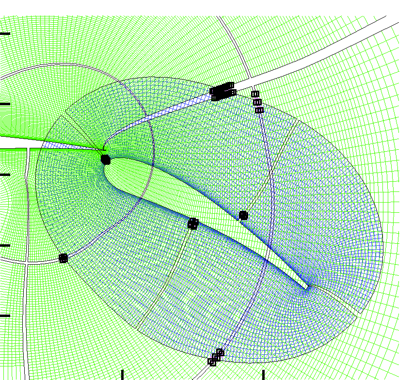
Distribution of interblock interpolation cells.

Figure 9.

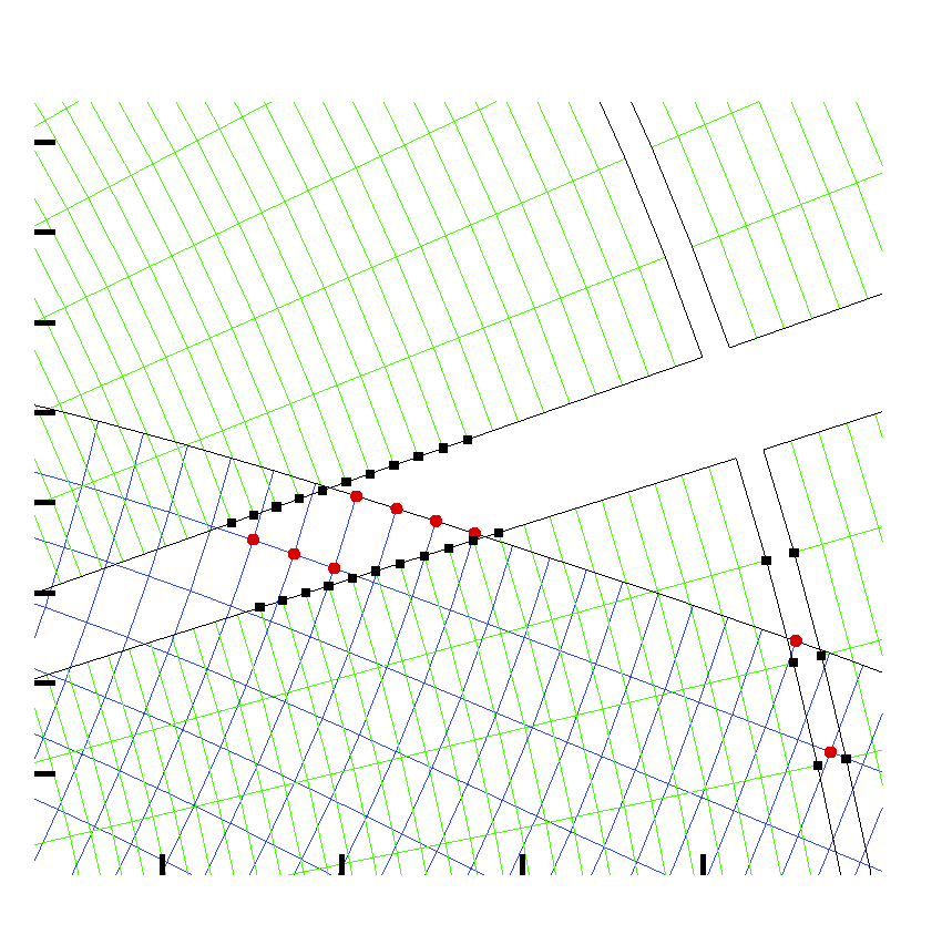
Closer view of interblock interpolation cells (circles: cell centers of the interpolated cells squares: cell centers of donor cells).

Figure 10 shows the pressure coefficients calculated by eight CPU cores in comparison with experiment data. Figure 12 shows Mach contours around 30P30N airfoil at steady state. It is shown in Figure 12 that it is clear to see the regions with low and high velocities and smooth flows. Figure 11 summarizes the convergence histories of lift, drag coefficients, and residual.

Figure 10.

Pressure coefficient comparisons.

Figure 11.

Convergence histories of lift, drag, and residual.

Figure 12.

Mach contours around 30P30N airfoil.

MBBOCO results

We used the wing–store ³¹ configuration for testing our MBBOCO approach. A multiblock overset mesh system with about total 57.3 million mesh cells was provided for the test. Table 1 shows the number of mesh blocks in the wing region and the store region.

Table 1.

Block parameters of the wing–store configuration.

Mesh cells: 57.3 million
Number of blocks	Wing blocks	Store blocks	One-to-one interfaces
4700	4309	391	14132

To demonstrate the advantages of the MBBOCO approach (called MB approach), we made a performance comparison between our approach and the process-based (PB) communication approach which avoided repeated communication among processes. However, the PB communication approach which is separate from the flow computations requires additional wall clock time.

Since the present MBBOCO takes place in pseudo-cycles, we performed 100 steps of steady calculations to analyze the performance. The real elapsed time (“wall clock time”) of a step was obtained by averaging the maximum duration at each step for the first 100 iterations. We selected the maximum duration among processes as the performance indicator because the slowest process determines the performance of the parallel simulation. Table 2 presents the real elapsed times for varying numbers of processes. Let comm_counts_MB denote the total number of sending operations in overlapping regions among all processes using MBBOCO and comm_counts_PB denote the same quantity using PB. These two values were collected by using a lightweight profiling library, called mpiP, ²⁸ for MPI programs. Figure 13 plots the ratio of comm_counts_MB to comm_counts_PB versus the number of processes.

Table 2.

Comparisons of real elapsed time (in seconds) for each implementation.

Number of processes	64	128	256	512	1024
MBBOCO	5.26	2.76	1.48	0.88	0.61
PB	5.40	2.86	1.57	0.96	0.72

MBBOCO: mesh block-based overset communication optimization; PB: process based.

Figure 13.

Communication counts comparison between MB and PB modes. MPI: message passing interface.

Figure 13 shows that comm_counts_MB increases 251%, 210%, 124%, 70%, and 56%, respectively, in comparison with comm_counts_PB as the number of processes increases from 64 to 1024. Although MB requires more data transmissions, Table 2 shows that the overall elapsed time obtained with MB mode has an advantage over PB mode. This is because the MPI operations and calculations were performed concurrently in MB mode and the communication overhead was hidden effectively by computations. Figure 13 also shows that the PB mode requires fewer MPI operations, but this advantage gradually decreases with increasing number of processes. Because as more processes are employed with a fixed number of mesh blocks, blocks are distributed more widely, which results in much more MPI operations in PB mode.

Because each block has to communicate with its neighbor blocks for data exchange, operations in communication usually involve almost over all processes. Unlike this kind of communication, data transmissions among overlapped regions in the overset mesh system (“Overset mesh system” section) occur in part of processes. This component of the MPI communication overhead varies from PTP due to uneven distribution of overlapped regions. The level of imbalance differs from case to case. Also, Table 2 shows that the communication overhead for overlapped regions depends, at least partially, on the number of processes, varying from 0.08 to 0.14 s. Therefore, communications within MB could be better tailored for arbitrary overset cases and numbers of processes.

Hybrid performance

We reused the wing–store case with a different block splitting method for evaluating the hybrid performance. We changed the wing–store mesh by allocating 2415 blocks of the 2641 total blocks to the wing region, with 226 in the store region. There were 8114 block-to-block interfaces in total. Unsteady MBS calculations were performed with each physical time step having 50 pseudo-cycles.

Figures 14 through 16 list the real elapsed times for a single pseudo-time step using the pure MPI and hybrid versions of the solver. The times listed in plots were computed by averaging the real elapsed times of 50 time steps on each process and selecting the maximum value from among all processes. We tested using 2, 4, and 8 OpenMP threads while considering specific numbers of processes.

Figure 14 shows that the hybrid version using 256 processes with varying numbers of OpenMP threads does not perform as well as the pure MPI version. This can be explained by the fact that computations with 256 processes already had a good load balance. Launching OpenMP threads added extra overhead. Another reason is that the overall amount of communication decreased as the number of processes decreased, but the elapsed time for communication on each process may increase due to the lack of communicational concurrency when fewer processes were launched.

Figure 14.

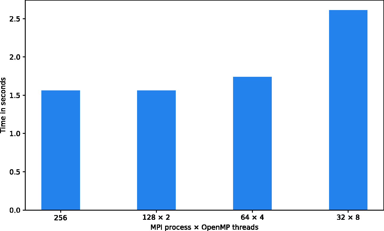
Hybrid performance comparison on 256 cores. MPI: message passing interface.

Figure 15 shows that results for the 256 × 2 (256 processes with each process 2 OpenMP threads) and 128 × 4 configurations outperformed the pure MPI version with 512 processes. Because the load balance factor, defined as the ratio of the maximum and average real elapsed times among processes, ⁴¹ becomes larger and using smaller number of processes produce relatively well load balance. Under these conditions, the OpenMP thread overhead is worthwhile. However, results with the 64 × 8 configuration were worse than the pure MPI version because parallel performance drops when more OpenMP threads were used. Furthermore, there was not enough computational workload on each mesh block with larger numbers of OpenMP threads. Figure 16 shows that the 128 × 8 configuration performed better than the pure MPI version. This is mainly explained by the fact that each process handled significantly fewer mesh blocks (average 2.57) such that the overall load balance deteriorated. The poor load balance was much improved by using only 128 processes but at the expense of poor scalability with 8 OpenMP threads.

Figure 15.

Hybrid performance comparison on 512 cores. MPI: message passing interface.

Figure 16.

Hybrid performance comparison on 1024 cores. MPI: message passing interface.

This investigation gives a solution for the case that there might not be enough mesh blocks for large-scale parallel computing and the hybrid MPI and OpenMP programming model could be considered to reduce the maximum wall clock time of a process.

The hybrid performance of parallel OMA on 128 and 256 processes is shown in Figures 17 and 18. The executing time of parallel OMA was divided into four parts: the time of hole cutting, the time of donor searching, the time of establishing octree search tree, and the time of MPI communication, respectively. In Figure 17, 2, 4, and 8 threads were launched on 128 processes, and the wall clock times of the first three parts were reduced by the multithreaded scheme. For hole cutting, since each process performed the same operation on hole mapping method to avoid extra MPI communication, which did not involve OpenMP thread, the acceleration effects on other code segments by OpenMP are not obvious as the number of threads increased. In Figure 18, a maximum number of four threads were investigated on up to 1024 cores. By comparing the performances of pure MPI results on 128 and 256 processes, the wall clock time did not decrease in proportion as the number of processes increased from 128 to 256. This is mainly because that the imbalance overlap regions result in imbalance donor searching task on each mesh block and the executing time in parallel environment is determined by the process that has the largest workload. The hybrid version showed that the overhead of donor searching can be reduced by employing multithreaded model without increasing the number of MPI processes. However, the scalability of octree decomposition by multithread is not as well as that by MPI, this is mainly caused by frequently memory operations in this part.

Figure 17.

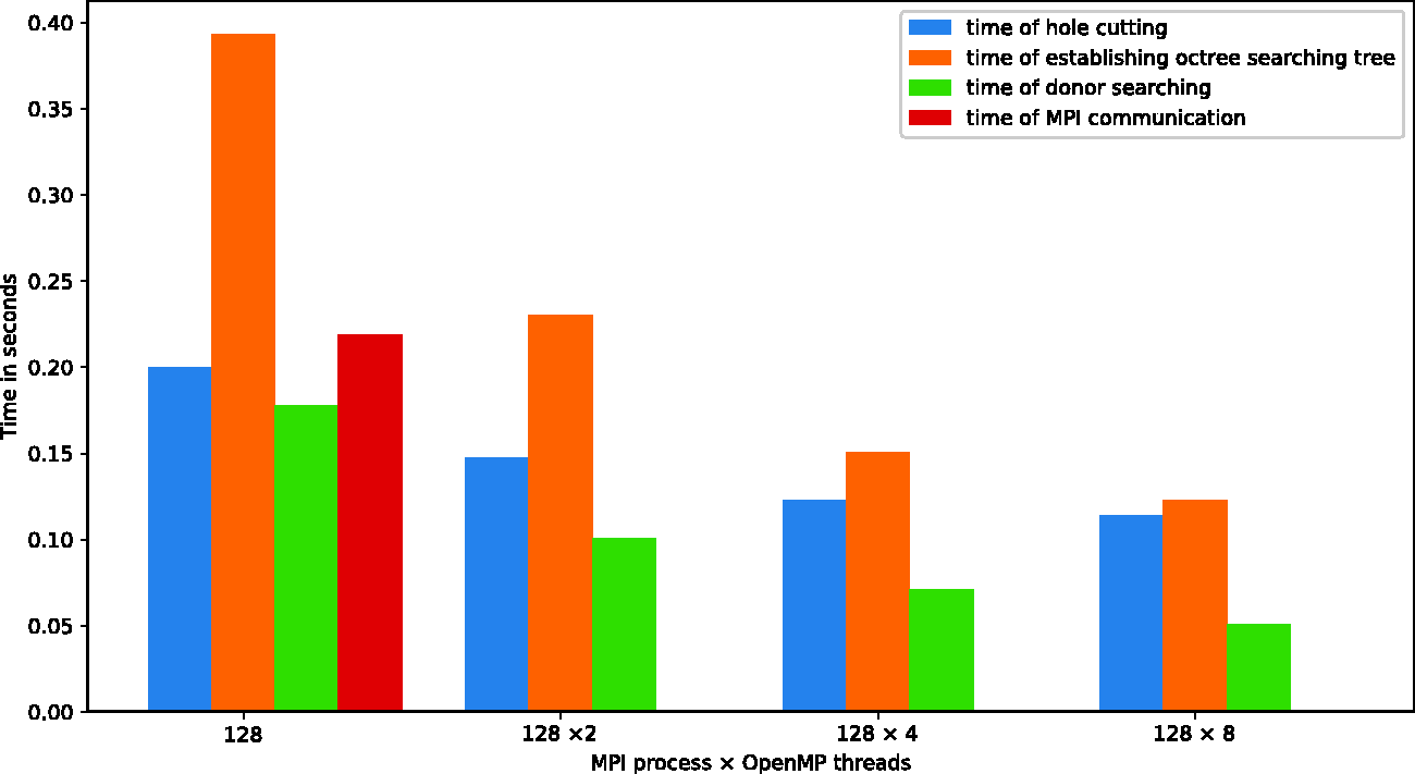
Hybrid performance for parallel OMA using 128 MPI processes. MPI: message passing interface.

Figure 18.

Hybrid performance for parallel OMA using 256 MPI processes. MPI: message passing interface.

We also evaluated the MPI communication time, which consists of the time to transfer donor search results to a target process, the time for identifying interblock interpolation cells, and the time to transfer donor search results back to the original process. The plots indicate that communication time varied little when going from 128 processors (0.219 s, 22.12%) to 256 (0.204 s, 27.98%) because the unbalanced search tasks for each process lead to unbalanced data transfer workloads. As mentioned in “Hybrid parallelization for OMA” section, there is no optimization of overlapped regions in the current version of OMA, so the parallel OMA accounts for less than 5% (depends on the number of pseudo-cycles) of the elapsed time of a single physical time step.

Simulation of wing–store case

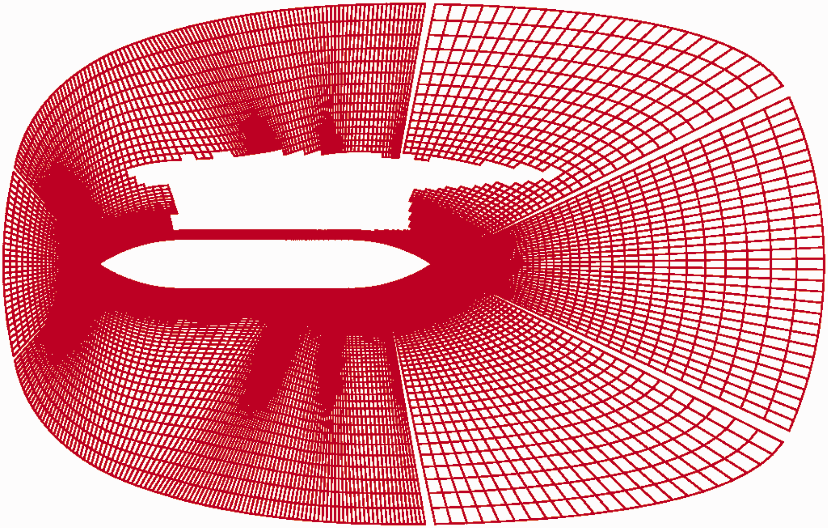
In this subsection, the wing–store case was used for parallel MBS computing. The initial mesh system contains 22 blocks and 4.8 million mesh cells. The block distribution of the walls is shown in Figure 19. The mesh assembly results are shown in Figures 20 to 22. Figure 20 shows the sectional view of hole cutting on the wing–mesh system. Figure 21 shows the sectional view of hole cutting on the store–mesh system. Figure 22 gives the overlapped mesh view at z = 3.302 plane obtained by parallel OMA.

Figure 19.

Blocks distribution of the initial wing–store configuration.

Figure 20.

Hole-cutting result on wing–mesh at z = 3.302.

Figure 21.

Hole-cutting result on store–mesh at z = 3.302.

Figure 22.

Overlapped mesh view at z = 3.302 after hole cutting.

The mesh system was doubled in all three directions and 410 mesh blocks were obtained (shown in Figure 23) by MST. 64 processes (not including the MPI host process) were launched with each process using 4 OpenMP threads. The unsteady time step was configured as Δt=0.64846 × 10⁻² and 55 steps with each conducts 50 pseudo-cycles were performed.

Figure 23.

Blocks distribution at walls after block splitting.

Figure 24.

Distance varying with time.

The steady solution of the case was obtained as the initial flow of the unsteady simulation. The unsteady simulation time was configured as about 0.35 s, and the store was configured by a forward and rear ejector force at the first 0.054 s. Therefore, the store began to separate from the wing body by the combination of aerodynamic force, gravity force, and ejector forces. Six parameters including distances, velocities, force coefficients, moment coefficients, attitude angles (Pitch, Yaw and Roll), and angular rates varying with times are shown in Figures 24 to 29. The results compare well with experiment data. It is seen from Figures 25 and 29 that the sharp change of velocity of W and angular rate of Wy at around 0.05 s indicates that the ejector forces are removed at that moment.

Figure 25.

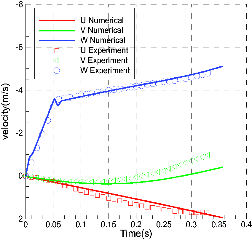
Velocities varying with time.

Figure 26.

Force coefficients varying with time.

Figure 27.

Moment coefficients varying with time.

Figure 28.

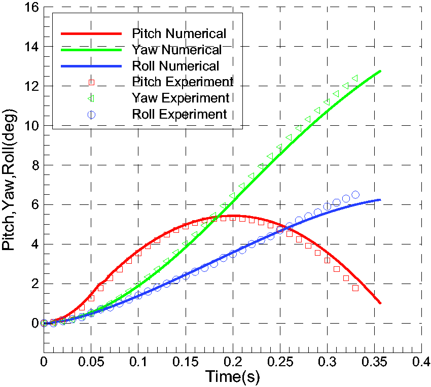
Pitch, yaw, roll varying with time.

Figure 29.

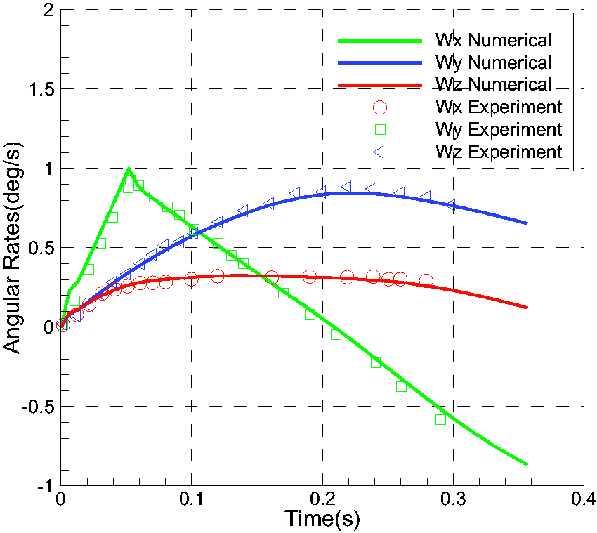
Angular rates varying with time.

During the unsteady calculations, seven instantaneous states, at t = 0 s (ns = 0), t = 0.064846 s (ns = 10), t = 0.129692 s (ns = 20), t = 0.194547 s (ns = 30), t = 0.259384 s (ns = 40), t = 0.32423 s (ns = 50), t = 0.356653 s (ns = 55) were captured, and the pressure distribution at ns = 30 and hole-cutting result on wing–mesh are shown in Figures 30 and 31, respectively. By using combined 64 MPI processes and 4 OpenMP threads (total 256 CPU cores), it took about 1.09 s to conduct a pseudo-time computing, 0.6 s to perform parallel OMA, and 0.2 s to update mesh and 6DOF equation solving. And it took about no more than 60 min to finish the simulation of the case.

Figure 30.

Pressure distribution at ns = 30.

Figure 31.

Hole-cutting result on wing–mesh at ns = 30.

Summary and future work

We have developed a hybrid MPI+OpenMP approach for MBS simulation with the implementation details of both the OMA and core of the numerical solver. And we have proposed and implemented a MBBOCO algorithm and shown the advantage over PB implementation by comparing their results on up to 1024 processor cores. By integrating the proposed algorithm into the hybrid approach, we have presented a standard wing–store separation case to validate the accuracy and performance of the implementations with 256 cores. Experiments have shown that the hybrid approach has an advantage in improving load balancing during parallel computing and provides a solution for large-scale computation with relatively fewer numbers of mesh blocks. Our work here is preliminary to our investigation into the possibility of performing MBS simulations on the Intel Many Integrated Core architecture. And we are currently working on a hybrid algorithm to optimize overlapping regions of the mesh assembler.