Sage Journals: Discover world-class research

Abstract

Faults can have significant, negative impacts on the operation and performance of simple and complex dynamic systems. Based on the integration of Bayesian network diagnostic features with Petri net formalism, the existing Bayesian-supported Petri net tool has demonstrated the flexibility of using the Petri net approach for diagnosing failure scenario of a dynamic system. However, studies on using the proposed hybrid Petri net approach for condition monitoring and early detection and diagnosis of single and multiple failures in a dynamic system with feedback control loops are yet to be investigated. Thus, this paper presents a methodology to address this research gap using the operation of a water tank level control system as a case study. The method combines the constructed Generalised Stochastic Petri Net (GSPN) model of the system operation with its corresponding fault diagnostic Petri net model, created using the proposed modified Bayesian Stochastic Petri Net (mBSPN) formalism. The GSPN model establishes the causal relationships between the system’s components and/or subsystems. It further identifies deviations in the sensor measurements of the observable process variables characterising the system operation. The information provided by the sensors in the system model are then inputted into the mBSPN model to diagnose the root cause of the observed deviations. The obtained results demonstrated the capability of using the proposed integrated Petri net methodology for system condition monitoring, early fault detection and diagnosis of single and multiple failures in a dynamic system with feedback control loops.

Keywords

Petri net Bayesian network fault diagnosis dynamic system inference algorithm

Introduction

Dynamic systems are systems whose states change over time. They are characterised by complex system topologies comprising many interacting units and equipment¹ such as component-to-component and subsystem-to-subsystem interactions. The high complexity of dynamic systems, including aircraft engines, nuclear reactors and safety critical systems found in many technological industries, means that the failure of one or more components of these systems can have significant negative impacts on the operation and overall performance of the system.^2–5 One way to detect and diagnose component failures is to use sensors to monitor the operational status of dynamic systems. However, using many sensors will increase cost and complicate the system.^6–8 Therefore, in addition to using a reasonable number of monitoring sensors, developing a technique to aid the rapid and accurate detection and diagnosis of the root cause of faults in a dynamic system is also crucial in order to prevent the probable consequences that may result in costly incidents such as loss of lives, fire outbreak, explosions and production lost.

Many approaches have been reported in the literature for system reliability modelling and fault diagnosis.⁹ Among these approaches, Bayesian Networks (BNs) and Petri Nets (PNs) have gained a wider adoption due to their strengths in modelling time, dependency and dynamic operations in detail. For example, BN uses conditional probabilities and Bayes theorem for modelling failure probability and fault diagnosis for a particular scenario. On the other hand, PNs and its variants, such as Generalised Stochastic Petri Nets (GSPN), are flexible modelling tools used to study the dynamic behaviour of complex systems. Unlike BN, which can be used in both predictive and diagnostic capacities,¹⁰ PNs lack the ability to model uncertainty directly or to compute the updated probability of a random variable given the observation of other specific variables.^11–13 Thus, this limits the modelling capacity of PN to mostly predictive analysis, similar to the failure analysis of the well-known conventional probabilistic approaches such as fault trees, reliability block diagrams and event trees, that is for computing system failure probability due to the failure of system components.

To address the aforementioned limitation of PN for fault diagnosis, some researchers have conducted studies whose primary aim is to enhance the modelling power of PN by incorporating probabilistic modelling features such as reasoning algorithms, conditional probability and Bayes theorem into Petri net formalisms. Among these studies are the works of Chiachío et al.,^11,14 Taleb-Berrouane et al.^15,16 and Zhou and Reniers¹⁶ who proposed the Plausible Petri Net (PPN), Bayesian Stochastic Petri Net (BSPN) and Probabilistic Petri Net (PPN) formalisms respectively, for modelling and analysing uncertainty, forward and backward reasonings. Despite the advantages of BNs over PNs for fault diagnosis, many discrete BNs, such as Discrete Dynamic BN (DDBN) proposed for diagnosing faults in complex dynamic systems, use the time-slice discretisation approach. However, using this approach negatively affects the computing time and accuracy of the fault diagnostic technique. In order to eliminate the need for time discretisation, a Generalised Continuous-Time BN (GCTBN) incorporating a continuous model of time was proposed by Codetta-Raiteri and Portinale.¹⁷ The GCTBN combined the strong features of both BNs and PNs to improve the performance of the fault diagnostic process.¹⁸

Andrews and Fecarotti¹⁹ combined the PN and BN approach in a method they named BP-Net, to investigate the safety effects of design and maintenance features on the performance of a remote unmanned wellhead platform operating over its design life. The proposed BP-Net is a model-to-model framework where PN was used to populate the conditional probability tables (CPT) in the developed BN model of the system. The proposed hybrid formalism overcomes limitations in conventional safety and risk analysis techniques, such as constant failure rates and the requirement of assuming independency among the system component failures. Taleb-Berrouane et al.¹⁵ also proposed a hybrid formalism known as Bayesian Stochastic Petri Net (BSPN) to enhance the modelling capabilities of Stochastic PN (SPN) by integrating the continuous data updating capabilities of BN with SPN. The efficiency of the BSPN formalism for fault diagnosis was examined on a simple system with one failure scenario (pump failure). Further work is required to investigate how the modelling tool could be extended for effective fault diagnosis of large-scale and complex systems characterised by feedback control loops and multiple failure scenarios.^20,21 However, for dynamic systems whose operational performance are monitored and controlled by a supervisory control system (sensors, controllers and actuators), many system component failures can lead to different unexpected system behaviour while the system is in operation. Besides, the presence of feedback control loop systems will further add complexity to the operational behaviour of the dynamic systems. Thus, this paper aims to propose a novel Petri net methodology suitable for condition monitoring and early detection and diagnosis of single and multiple failure scenarios in a complex dynamic system. The methodology is based on the fusion of Generalised Stochastic Petri Net (GSPN) model of the system operation with its fault diagnostic Petri net model, developed using the proposed modified Bayesian Stochastic Petri Net (mBSPN) approach. The modelling capability of the GSPN-mBSPN methodology was examined on a water tank level system whose operating conditions are monitored and controlled by the feedback control loop systems located at some sections of the system. The contributions of this paper can be summarised as follows:

(i) An integrated system operation and fault diagnostic Petri net methodology for single and multiple faults diagnosis in a dynamic system with control loops is proposed.

(ii) Proposition of new Petri net modelling features for further improvement on the modelling powers of Generalised Stochastic Petri net and Bayesian Stochastic Petri net formalisms for studying the reliability and fault diagnosis of complex dynamic systems with feedback control loops is made.

(iii) The results show the accuracy of using the proposed integrated Petri net methodology (GSPN-mBSPN) for single and multiple faults diagnosis in a complex dynamic system.

The remainder of the paper is structured as follows. Section 2 presents details of the methodology for the condition monitoring and early detection and diagnosis of failures in a dynamically controlled system. Steps of the methodology, such as the integration of the system operation and fault diagnostic models, Monte Carlo Simulation output analysis of the integrated model are described in detail. The application of the proposed methodology to water tank level control system is discussed in Section 3. Lastly, Section 4 gives the conclusion and a review for future work.

Proposed methodology

Figure 1 depicts the main steps of the Petri net methodology for the condition monitoring and early detection and diagnosis of faults in a dynamic system proposed in this paper. Each step is described in detail in the following sub-sections.

Figure 1.

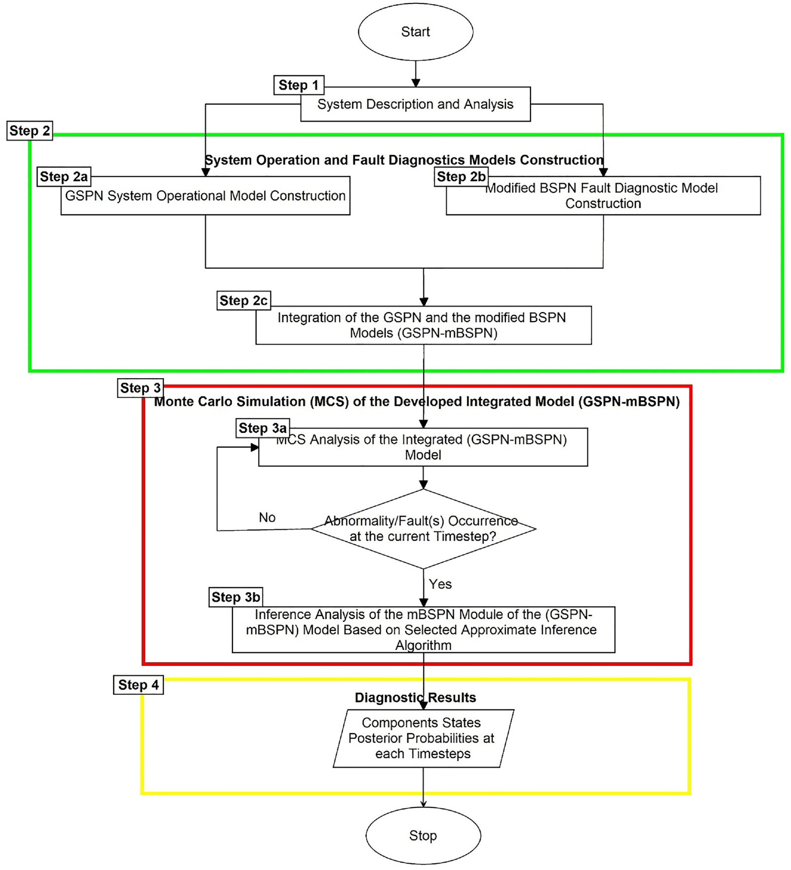
Proposed methodological framework for fault detection and diagnosis of dynamic systems.

Step 1: System description and analysis

The system is studied to identify its structure, functional behaviour, operating states/modes, information about the states/modes (working and failure) and the failure data of components that make up the system for the purpose of defining actions and interactions among the system components, including the monitoring components (sensors) deployed on the system.

Step 2: System operational and fault diagnostic PN module construction

When modelling complex dynamic systems, sectional and component-based approaches are often employed, as described in the works of Bartlett et al.^22,23 and Remenyte-Prescott and Andrews.²³ A typical illustration of such an approach is depicted in Figure 2. The system is first divided into sections/subsystems comprised of two or more components such that each one of the sections only affects a single system process variable (e.g. flow or level). A component PN model describing the component’s normal working and failure state/mode(s) is developed for each component that makes up the section. After that, an operational propagation PN model is constructed to establish an input-output dependency structure among connected components in a section. The dependency model structures are developed considering the normal working and failure state/modes of the connected components in the section. All the section models are combined to produce an overall system operation model. Within the system’s operational GSPN model, sensor observation and fault detection PN models are developed to detect faults or anomalies while the system is in operation. In the event of unexpected system behaviour, a fault diagnostic PN module based on modified BSPN (mBSPN) would be triggered to analyse the cause of any abnormality observed in the system.

Figure 2.

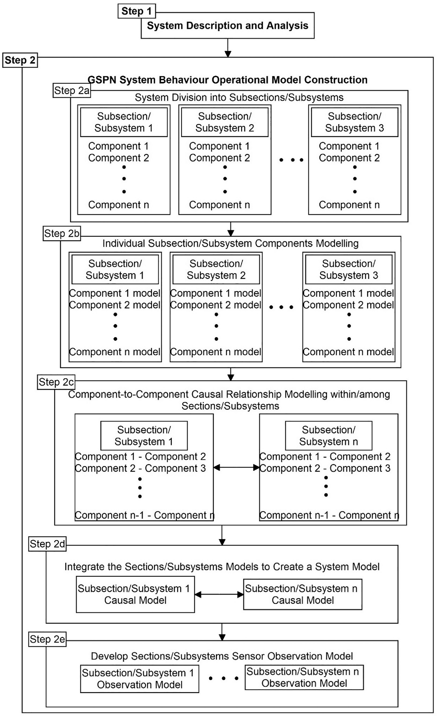
Framework for constructing system operational PN model for a dynamic system.

Overview of the GSPN-mBSPN approach

The conventional GSPN formalism²⁴ is an extension of a Stochastic Petri Net with ‘inhibitor arcs’ and ‘immediate transitions’. The formal definitions and the descriptions of the elements of the GSPN formalism used in this paper are given in the work of Nourredine et al.²⁵ Despite the usefulness of the GSPN formalism and other extended PN features proposed in the literature,^9,14,20,26 such as different arc and place types and their corresponding transition types and firing rules, they have limitations in modelling the condition, early fault detection and diagnostic processes of a dynamic system with feedback control loops. To address this limitation, additional PN features such as conditional output reset place (CORP), arc (COA), transition (CRT), conditional probabilistic transitions (CPT) and new firing rules are introduced to extend the standard GSPN approach.

In addition, BSPN is one of the new PN extensions proposed by Taleb-Berrouane et al.¹⁵ It is a Stochastic Petri Net model extended with Bayesian Network (BN) features such as conditional probabilities, Bayes theorem and data updating features. BSPN supports the use of the PN approach for fault diagnosis. Details on the methodology for converting a BN graph to a BSPN model can be found in the literature.¹⁵ Motivated by the work of Taleb-Berrouane et al.,¹⁵ the primary aim of this paper is to propose an integrated Petri net method for the detection and diagnosis of abnormalities or faults in a dynamic system with feedback control loops by incorporating inference sampling algorithms of a Bayesian network in a GSPN system simulation model. To achieve this aim, new probabilistic transition types (Independent and Dependent Non-Observable and Observable Conditional Probabilistic Transitions; ICPT, DCPT and DCPT^*), firing rule, places and arc types (evidence places and arcs) are further proposed in this paper. These new features make it possible to use an integrated Petri net model based on GSPN and modified BSPN approaches for condition monitoring, fault detection and diagnosis of a dynamic system with feedback controls during the system operation. Table 1 shows the graphical representations and descriptions of the proposed new PN features together with the existing Petri net symbols essential for modelling operational behaviour and fault diagnostic processes of a dynamic system with feedback control loops using GSPN-mBSPN approach.

Table 1.

Description of standard and new Petri net symbols.

Petri net symbol	Name
	Immediate transition
	Deterministic/stochastic transition
	Conditional reset transition (CRT)^a
	Conditional probabilistic transition (CPT)^a. That is $T_{ICPT}$ , $T_{DCPT}$ and $T_{DCP T^{*}}$
	Place
	Token
	Normal input/output arc
	Inhibitor arc
	Test arc
	Reset arc
	Causal arc
	Evidence arc (EA)^a
	Conditional output arc (COA)^a
	Conditional output arc and reset arc (CORA)^a
	Conditional probabilistic arc (CPA)^a

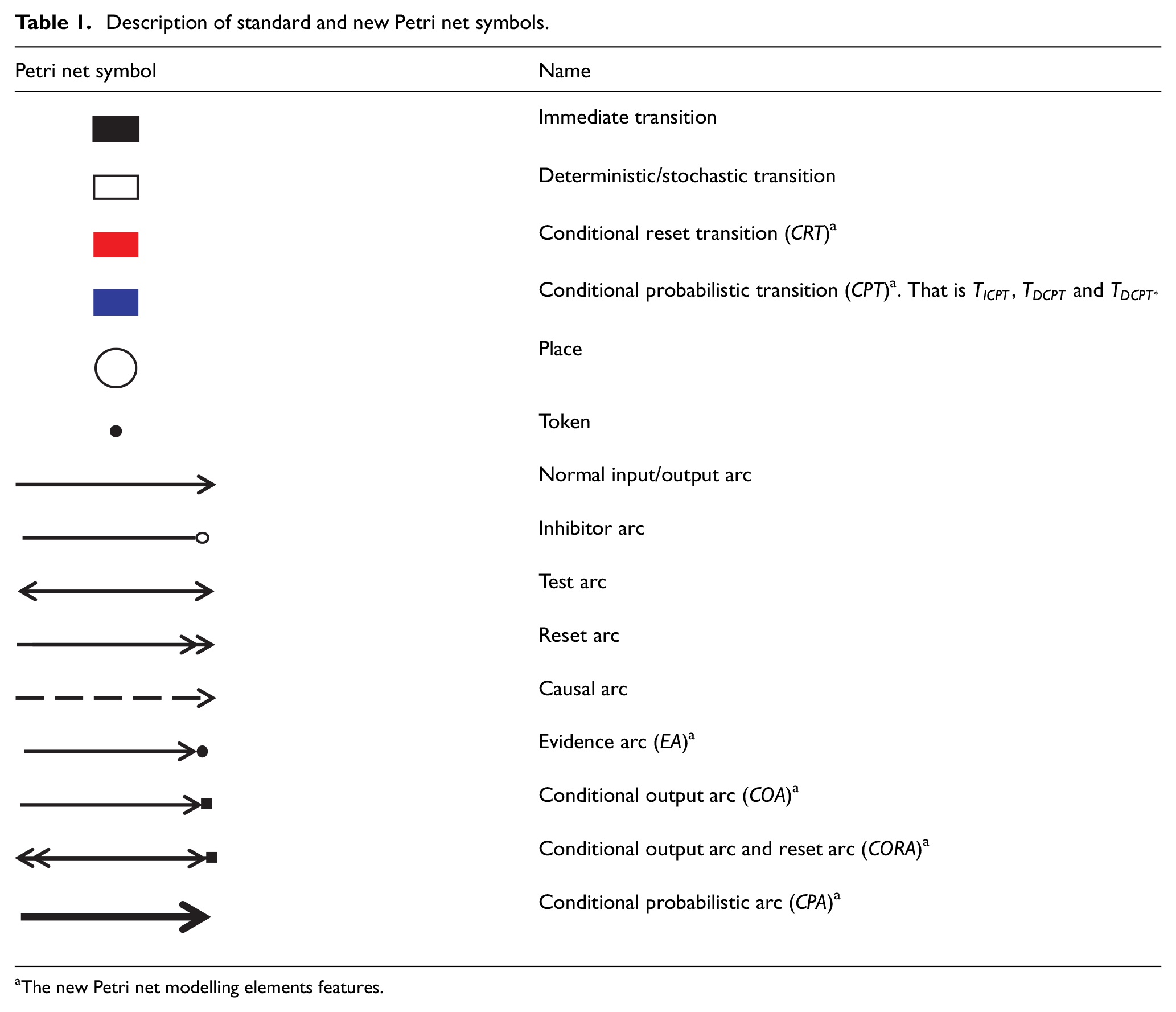
The new Petri net modelling elements features.

Formal definition of the GSPN-mBSPN approach

A formal definition of the GSPN-mBSPN methodology is presented in definition 1 while the definition of the enabling and firing rules of the new transition types in a GSPN-mBSPN are explained in definitions 2 and 3.

Definition 1. A GSPN-mBSPN method is defined as $GSPN - mBSPN = {GSPN, P_{TP}, A_{TA}, P_{CORP},$ $P_{COP}, T_{CRT}, InferenceCode, A_{RA}, mBSPN, A_{COA}}$ such that:

1. $GSPN$ is the conventional Generalised Stochastic Petri Net formalism for describing the operational behaviour of a dynamic system. This formalism is adopted and defined in Nourredine et al.²⁵

2. $P_{TP}$ is a set of test places in the GSPN-mBSPN model that enhance the modelling efficiency of Petri net models, particularly in complex systems. For example, they are used to test components’ states and system/subsystems’ states/conditions in a Petri net model of a dynamic system.

3. $A_{TA}$ is a set of test arcs such that $a_{INA} (p_{INP} \in P, t \in T) = a_{OUTA} (t, p_{OUTP} \in P)$ and $p_{INP} (t)$ $p_{INP} (t) = p_{OUTP} (t)$ where $a_{INA} (p_{INP}, t)$ is the weight of the input arc from the input place $p_{INP}$ to the transition $t$ , and $a_{OUT} (t, p_{OUTP})$ is the weight of the output arc from transition $t$ to the output place $p_{OUTP}$ . Thus, for simplicity, mathematically $a_{INA} (t) = a_{OUTA} (t)$ and $p_{INP} (t) = p_{OUTP} (t)$ are denoted by $p_{TP} (t)$ and $a_{TA} (t)$ respectively, such that $p_{TP} (t) \in P_{TP}$ and $a_{TA} (t) \in A_{TA}$ .

4. $P_{CORP}$ is a set of conditional output reset places. This special type of reset place²⁷ acts as the interface for passing observed evidence from the system behavioural GSPN module of GSPN-mBSPN to its fault diagnostic mBSPN module.

5. $P_{COP}$ is a set of places known as conditional output/trigger places. These places trigger the fault diagnostic module when an abnormality is detected during system operation.

6. $T_{CRT}$ represents a set of conditional reset transitions, a special type of reset transition. $T_{CRT}$ is utilised to model fault detection when the system operating state deviates from its expected normal conditions.

7. $InferenceCode \to {1, 2, 3}$ denotes the codes for the applied Bayesian inference sampling algorithms,²⁸ such that $InferenceCode = 1, 2, 3$ denote forward/prior sampling, rejection sampling and likelihood weighting sampling respectively.

8. $A_{RA}$ is a set of reset arcs where $a_{RA} (p_{CORP}, t_{CRT})$ is the weight of the reset arc from the conditional output reset place $p_{CORP}$ to the conditional reset transition $t_{CRT}$ .

9. $mBSPN$ is a fault diagnostic Petri net module of the GSPN-mBSPN method, formally defined as $m B S P N = (P^{d}, T_{C P T}^{d}, T y p e_{t_{C P T}^{d}}, F_{c p t}, I n f e r e n c e C o d e, A^{d})$ , where:

a. $P^{d}$ is a set of places in the fault diagnostic module. $P^{d} = P_{INP}^{d} \cup_{CPP}^{d} \cup_{CP}^{d} \cup_{EP}^{d}$ and $P_{INP}^{d}, P_{CPP}^{d}, P_{CP}^{d}, P_{EP}^{d}$ are sets of input, conditional probabilistic, causal and evidence places such that ${(P_{INP}^{d} \subseteq P_{COP}) \land (P_{EP}^{d} \subseteq P_{CORP}) \land (P_{CPP} \subseteq P_{OUTP}^{d})}$ . $P_{OUTP}^{d}$ is the set of output places of the transitions in the fault diagnostic module.

b. $T_{CPT}^{d}$ is a set of conditional probabilistic transitions and $Typ e_{t_{CPT}^{d}}$ is a function that assigns a type to a $t_{CPT}^{d} \in T_{CPT}^{d}$ transition. $T_{CPT}^{d} =$ $T_{C P T_{I C P T}}^{d} \cup T_{C P T_{D C P T^{*}}}^{d} \cup T_{C P T_{D C P T}}^{d}$ such that $T_{CP T_{ICPT}}^{d},$ $T_{CP T_{DCP T^{*}}}^{d}$ and $T_{CP T_{DCPT}}^{d}$ are sets of independent, dependent observable and dependent non-observable types of $T_{CPT}^{d}$ transitions respectively. They represent system components, propagated system operational variables and states of monitoring components in the operational GSPN model of a dynamic system.

c. $F_{cpt}$ is a function that assigns a conditional probability table to a transition $t_{CPT}^{d}$ : $t_{CPT}^{d} \to cp t_{t_{CPT}^{d}}$ .

d. $InferenceCode$ is as defined in (7)

e. $A^{d}$ is a set of arcs in the fault diagnostic module. $A^{d} = A_{I N A}^{d} \overset{A_{C A}^{d}}{\cup} \overset{A_{E A}^{d}}{\cup} \overset{A_{C P A}^{d}}{\cup}$ and $A_{INA}^{d}, A_{CA}^{d}, A_{EA}^{d}$ and $A_{CPA}^{d}$ are sets of input, causal, evidence and conditional probabilistic arcs such that $A_{INA}^{d} (P_{INP}^{d} x T_{CPT}^{d})$ , $A_{CA}^{d} (P_{CPP}^{d} (T_{CPT}^{d} \ {T_{CP T_{DCP T^{*}}}^{d}}) x T_{CPT}^{d} \ {T_{CP T_{ICPT}}^{d}})$ , $A_{E A}^{d} (P_{E P}^{d} x T_{C P T_{D C P T^{*}}}^{d})$ and $A_{CPA}^{d} (T_{CPT}^{d} x P_{CPP}^{d})$ are sets of arcs between places $P_{INP}^{d}$ and transitions $T_{CPT}^{d}$ , places $P_{CPP}^{d}$ of transitions $T_{CPT}^{d}$ except for transitions $T_{CP T_{DCP T^{*}}}^{d}$ and transitions $T_{CPT}^{d}$ except for transitions $T_{C P T_{I C P T}}^{d}$ , places $P_{EP}^{d}$ and transitions $T_{C P T_{D C P T^{*}}}^{d}$ and transitions $T_{CPT}^{d}$ and places $P_{CPP}^{d}$ , respectively. The corresponding arc weights for the sets of arcs are given by:

i. An $a_{INA}^{d} \in A_{INA}^{d}$ arc weight is a function: $a_{t_{INA}}^{d} = {1 : a_{INA}^{d} (p_{INP}^{d} x t_{CPT}^{d})}$ ,

ii. An $a_{CA}^{d} \in A_{CA}^{d}$ arc weight is a function: $a_{t_{CA}}^{d} = {n : n \to {0, 1}, n = m (p_{CPP}^{d}), 0 \leq m (p_{CPP}^{d})$ $\leq 1, p_{CPP}^{d} \in P_{CPP}^{d} (t_{CPT}^{d} \ t_{CP T_{DCP T^{*}}}^{d}), t_{CPT}^{d} \ t_{CP T_{ICPT}}^{d}}$ , where $m (p_{CPP}^{d})$ is the current marking of the place $p_{CPP}^{d}$ from the transition $t_{CPT}^{d} \ t_{CP T_{DCP T^{*}}}^{d}$ to a transition $t_{CPT}^{d} \ t_{CP T_{ICPT}}^{d}$ .

iii. An $a_{EA}^{d} \in A_{EA}^{d}$ arc weight is a function: $a_{t_{E A}}^{d} = {n \in ℕ : n = m (p_{E P}^{d}), 1 \leq m (p_{E P}^{d}) \leq | P_{C P P}^{d} (t_{C P T_{D C P T^{*}}}^{d}) |}$ , where $m (p_{EP}^{d})$ is the current marking of the evidence place $p_{EP}^{d}$ and $| P_{CPP}^{d} (t_{CP T_{DCP T^{*}}}^{d}) |$ is the cardinality of the set $P_{CPP}^{d}$ of the transition $t_{CP T_{DCP T^{*}}}^{d}$ . Generally, $| P_{CPP}^{d} (t_{CPT}^{d}) |$ is equivalent to the total number of places denoting the system component states, states of a propagated system operational variable or monitoring component states in the operational GSPN model of a dynamic system.

iv. An $a_{CPA}^{d} (t_{CPT}^{d}) \in A_{CPA}^{d}$ arc weight is a function: $a_{t_{C P A}}^{d} = {n : n \to {0, 1}, g (I n f e r e n c e C o d e, c p t_{t_{C P T}^{d}},$ $a_{C A}^{d} (t_{C P T}^{d}), a_{E A}^{d} (t_{C P T}^{d})) = i, i < | P_{C P P}^{d} (t_{C P T}^{d}) |}$ . $g (InferenceCode, cp t_{t_{CPT}^{d}}, a_{CA}^{d} (t_{CPT}^{d}), a_{EA}^{d} (t_{CPT}^{d}))$ is an inference sampling algorithm function to compute the index of a sample state from the states of a component, propagated variable or monitoring component based on the selected inference algorithm such that if $g (I n f e r e n c e C o d e, c p t_{t_{C P T}^{d}}, a_{C A}^{d} (t_{C P T}^{d}), a_{E A}^{d} (t_{C P T}^{d})) = i$ and $i = indexof (p_{CPP}^{d})$ in the vector of $P_{CPP}^{d} (t_{CPT}^{d})$ then, $n = 1$ and $0$ otherwise.

10. $A_{COA}$ : a set of conditional output arcs between $T_{CRT}$ and $P_{CORP}$ or between $T_{CRT}$ and $P_{COP}$ . That is $A_{COA} = {A_{COA} (T_{CRT} x P_{CORP}) \cup A_{COA}$ $(T_{CRT} x P_{COP})}$ . $a_{C O A} (t_{C R T} \in T_{C R T}, p_{C O R P} \in P_{C O R P})$ and $a_{COA} (t_{CRT}, p_{COP} \in P_{COP})$ are the weights of $a_{COA} (t_{CRT} x p_{CORP})$ and $a_{COA} (t_{CRT} x p_{COP})$ , respectively and defined as:

a. $a_{COA} (t_{CRT}, p_{CORP}) = {\begin{matrix} 0 if InferenceCode = 1 \\ {i + 1 | 0 \leq i < | P_{CPP}^{d} (t_{CP T_{DCP T^{*}}}^{d}) |} Otherwise \end{matrix}$ ,

where $i$ is the index of the $p_{CPP} (t_{CP T_{DCP T^{*}}}^{d})$ with evidence in the vector of the conditional probabilistic places of transition $t_{CPT}^{d}$ (i.e. $P_{CPP}^{d} (t_{CPT}^{d})$ ) such that $p_{C O R P} \to e_{E P} (t_{C P T_{D C P T^{*}}}^{d})$ where $e_{E P} (t_{C P T_{D C P T^{*}}}^{d})$ is the evidence place of the transition $t_{CP T_{DCP T^{*}}}^{d}$ .

b. $a_{COA} (t_{CRT}, p_{COP}) = {\begin{matrix} 1 if m (p_{COP} (t_{CPT}^{d})) = 0 \\ 0 Otherwise \end{matrix}$ , where $m (p_{COP} (t_{CPT}^{d}))$ is the current marking of the conditional output place $p_{COP}$ of transition $t_{CPT}^{d}$ .

Enableness and firing rules of transitions in the GSPN-mBSPN

The definition of the enabling and firing rules of the new transitions types in the GSPN-mBSPN are explained in definitions 2 and 3.

Definition 2. The enableness of a transition $t$ in the GSPN-mBSPN is governed by the following conditional expression.

$Enableness (t) = {\begin{matrix} True if \forall p \in (P_{INP} (t) \lor P_{TP} (t)), M (p) \geq a (p x t) \in (a_{INA} \lor a_{TA}) \\ True if \forall p \in P_{INHP} (t), M (p) < a (p x t) \in a_{INHA} \\ False Otherwise \end{matrix}$ , where $a_{INHA}$ is the inhibitor arc between the inhibitor place $P_{INHP}$ and transition $t$ .

Definition 3. Due to the flexibility of Petri net formalisms, the standard firing rule for an enabled transition $t$ may change if extra conditions are considered. This is the case for the proposed CRT and CPT transitions, where additional information is required for firing the transitions. In general, the firing of a transition $t$ in a GSPN-mBSPN model will change the markings of some places in the net depending on the transition and place types. For the standard transitions, such as immediate ( $T_{IMT}$ ), stochastic ( $T_{STT}$ ) and deterministic ( $T_{DET}$ ) transitions, the conventional transition firing rules in a $GSPN$ formalism are conserved. However, given a generalised structure of a fault detection module within a GSPN module of a GSPN-mBSPN, as depicted in Figure 3, the defined firing rule of a conditional reset transition $t_{CRT}$ is given as follows:

firing (t_{CRT}) : {\begin{matrix} M^{'} (p) = M (p) - a_{RA} (p, t) + a_{COA} \\ (t, p) \forall p \in P_{CORP} (t) \\ M^{'} (p) = M (p) + a_{COA} (t, p) \\ \forall p \in P_{COP} (t) \end{matrix}

where $M^{'} (p)$ and $M (p)$ are the updated and the initial marking of place $p$ .

Figure 3.

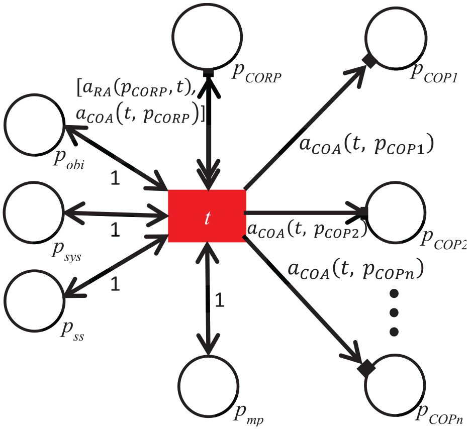
A generalised structure of a fault detection module of a GSPN-mBSPN.

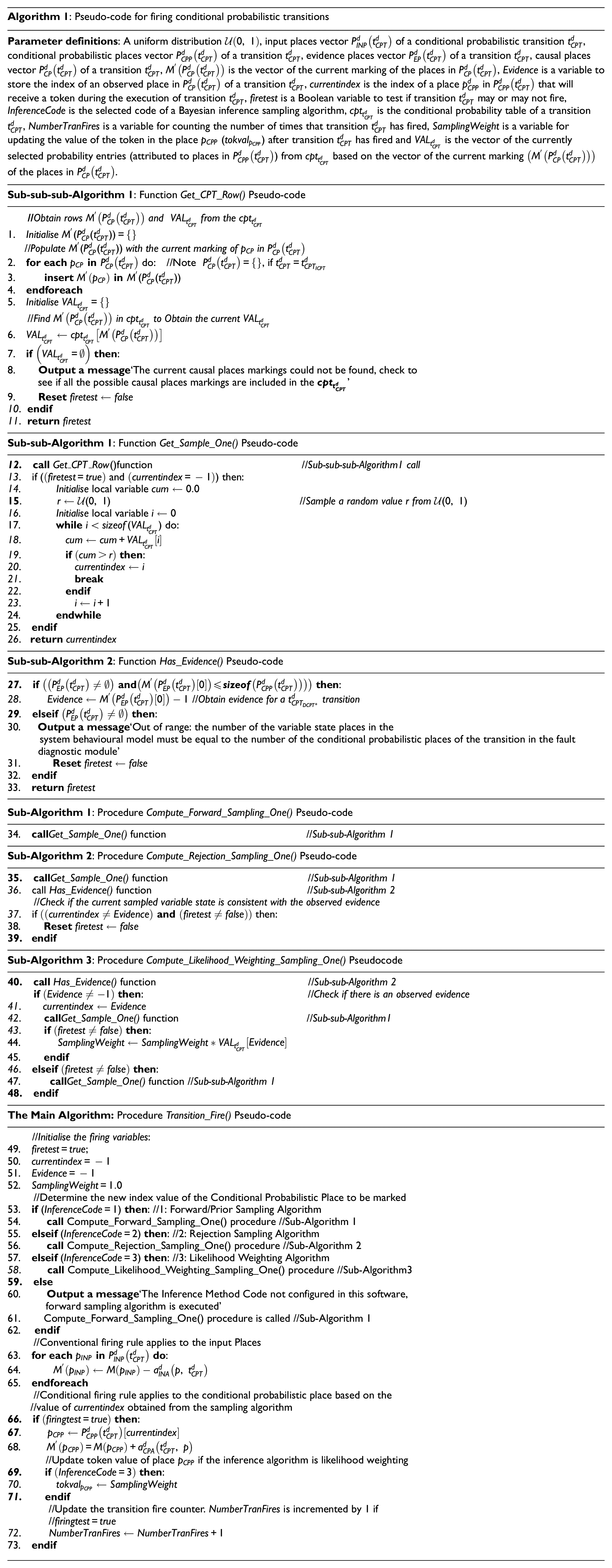
Places p_obi, p_sys, p_mp and p_ss in Figure 3 symbolise the time interval of sensor observation, the system state, the abnormal state of the monitoring parameter and the state of the sensor related to p_mp. Compared to the CRT transition, the firing rule of a CPT transition is more complex because it depends on the type of the CPT transition and the selected inference sampling algorithm. Thus, the generalised structures of the CPT transitions in the fault diagnostic module (mBSPN) of a GSPN-mBSPN are as depicted in Figure 4. At the same time, the defined firing rule for the different types of CPT transitions in the mBSPN module of a GSPN-mBSPN is given by the pseudo-code in Algorithm 1. As shown in Figure 4, suppose t2 is a distinct operational process that depends on the states of a component represented by the CPT transition t1. 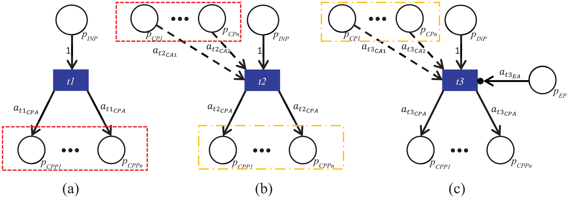Then, the causal places $(P_{CP})$ of t2 will be the same as the conditional probabilistic places ( $P_{CPP}$ ) of t1. Likewise, if t3 depends on t2, then $P_{CP} (t 3)$ will be equal to $P_{CPP} (t 2)$ .

Figure 4.

Generalised structure of: (a) independent conditional probabilistic transition, (b) dependent non-observable conditional probabilistic transition and (c) dependent observable conditional probabilistic transition.

Algorithm 1: Pseudo-code for firing conditional probabilistic transitions
Parameter definitions: A uniform distribution $U (0, 1)$ , input places vector $P_{INP}^{d} (t_{CPT}^{d})$ of a conditional probabilistic transition $t_{CPT}^{d}$ , conditional probabilistic places vector $P_{CPP}^{d} (t_{CPT}^{d})$ of a transition $t_{CPT}^{d}$ , evidence places vector $P_{EP}^{d} (t_{CPT}^{d})$ of a transition $t_{CPT}^{d}$ , causal places vector $P_{CP}^{d} (t_{CPT}^{d})$ of a transition $t_{CPT}^{d}$ , $M^{'} (P_{CP}^{d} (t_{CPT}^{d}))$ is the vector of the current marking of the places in $P_{CP}^{d} (t_{CPT}^{d})$ , $Evidence$ is a variable to store the index of an observed place in $P_{CP}^{d} (t_{CPT}^{d})$ of a transition $t_{CPT}^{d}$ , $currentindex$ is the index of a place $p_{CPP}^{d}$ in $P_{CPP}^{d} (t_{CPT}^{d})$ that will receive a token during the execution of transition $t_{CPT}^{d}$ , $firetest$ is a Boolean variable to test if transition $t_{CPT}^{d}$ may or may not fire, $InferenceCode$ is the selected code of a Bayesian inference sampling algorithm, $cp t_{t_{CPT}^{d}}$ is the conditional probability table of a transition $t_{CPT}^{d}$ , $NumberTranFires$ is a variable for counting the number of times that transition $t_{CPT}^{d}$ has fired, $SamplingWeight$ is a variable for updating the value of the token in the place $p_{CPP}$ ( $tokva l_{p_{CPP}}$ ) after transition $t_{CPT}^{d}$ has fired and $VA L_{t_{CPT}^{d}}$ is the vector of the currently selected probability entries (attributed to places in $P_{CPP}^{d} (t_{CPT}^{d})$ ) from $cp t_{t_{CPT}^{d}}$ based on the vector of the current marking $(M^{'} (P_{CP}^{d} (t_{CPT}^{d})))$ of the places in $P_{CP}^{d} (t_{CPT}^{d})$ .
Sub-sub-sub-Algorithm 1: Function Get_CPT_Row() Pseudo-code
// Obtain rows $M^{'} (P_{CP}^{d} (t_{CPT}^{d}))$ and $VA L_{t_{CPT}^{d}}$ from the $cp t_{t_{CPT}^{d}}$ 1. Initialise $M^{'} (P_{CP}^{d} (t_{CPT}^{d})) = {}$ //Populate $M^{'} (P_{CP}^{d} (t_{CPT}^{d}))$ with the current marking of $p_{CP}$ in $P_{CP}^{d} (t_{CPT}^{d})$ 2. for each $p_{CP} in P_{CP}^{d} (t_{CPT}^{d})$ do: //Note $P_{CP}^{d} (t_{CPT}^{d}) = {}$ , if $t_{CPT}^{d} = t_{CP T_{ICPT}}^{d}$ 3. insert $M^{'} (p_{CP}) in M^{'} (P_{CP}^{d} (t_{CPT}^{d}))$ 4. endforeach 5. Initialise $VA L_{t_{CPT}^{d}} = {}$ //Find $M^{'} (P_{CP}^{d} (t_{CPT}^{d}))$ in $cp t_{t_{CPT}^{d}}$ to Obtain the current $VA L_{t_{CPT}^{d}}$ 6. $VA L_{t_{CPT}^{d}} \leftarrow cp t_{t_{CPT}^{d}} [M^{'} (P_{CP}^{d} (t_{CPT}^{d}))]$ 7. if $(VA L_{t_{CPT}^{d}} = \emptyset)$ then: 8. Output a message‘The current causal places markings could not be found, check to see if all the possible causal places markings are included in the $cp t_{t_{CPT}^{d}}$ ’ 9. Reset $firetest \leftarrow false$ 10. endif 11. return $firetest$
Sub-sub-Algorithm 1: Function Get_Sample_One() Pseudo-code
12. call $Get_CPT_Row ()$ function //Sub-sub-sub-Algorithm1 call 13. if ( $(firetest = true)$ and $(currentindex = - 1)$ ) then: 14. Initialise local variable $cum \leftarrow 0.0$ 15. $r \leftarrow U (0, 1)$ //Sample a random value $r$ from $U (0, 1)$ 16. Initialise local variable $i \leftarrow 0$ 17. while $i < sizeof (VA L_{t_{CPT}^{d}})$ do: 18. $cum \leftarrow cum + VA L_{t_{CPT}^{d}} [i]$ 19. if $(cum > r)$ then: 20. $currentindex \leftarrow i$ 21. break 22. endif 23. $i \leftarrow i + 1$ 24. endwhile 25. endif 26. return $currentindex$
Sub-sub-Algorithm 2: Function Has_Evidence() Pseudo-code
27. if $((P_{EP}^{d} (t_{CPT}^{d}) \neq \emptyset) and (M^{'} (P_{EP}^{d} (t_{CPT}^{d}) [0]) \leq sizeof (P_{CPP}^{d} (t_{CPT}^{d}))))$ then: 28. $Evidence \leftarrow M^{'} (P_{EP}^{d} (t_{CPT}^{d}) [0]) - 1$ //Obtain evidence for a $t_{CP T_{DCP T^{}}}^{d}$ transition* 29 . elseif $(P_{EP}^{d} (t_{CPT}^{d}) \neq \emptyset)$ then: 30. Output a message‘Out of range: the number of the variable state places in the system behavioural model must be equal to the number of the conditional probabilistic places of the transition in the fault diagnostic module’ 31. Reset $firetest \leftarrow false$ 32. endif 33. return $firetest$
Sub-Algorithm 1: Procedure Compute_Forward_Sampling_One() Pseudo-code
34. callGet_Sample_One() function //Sub-sub-Algorithm 1
Sub-Algorithm 2: Procedure Compute_Rejection_Sampling_One() Pseudo-code
35. call Get_Sample_One() function //Sub-sub-Algorithm 1 36. call Has_Evidence() function //Sub-sub-Algorithm 2 //Check if the current sampled variable state is consistent with the observed evidence 37. if $((currentindex \neq Evidence) and (firetest \neq false))$ then: 38. Reset $firetest \leftarrow false$ 39. endif
Sub-Algorithm 3: Procedure Compute_Likelihood_Weighting_Sampling_One() Pseudocode
40. call Has_Evidence() function //Sub-sub-Algorithm 2 if $(Evidence \neq - 1)$ then: //Check if there is an observed evidence 41. $currentindex \leftarrow Evidence$ 42. callGet_Sample_One() function //Sub-sub-Algorithm1 43. if $(firetest \neq false)$ then: 44. $SamplingWeight \leftarrow SamplingWeight * VA L_{t_{CPT}^{d}} [Evidence]$ 45. endif 46. elseif $(firetest \neq false)$ then: 47. callGet_Sample_One() function //Sub-sub-Algorithm 1 48. endif
The Main Algorithm: Procedure Transition_Fire() Pseudo-code
//Initialise the firing variables: 49. $firetest = true$ ; 50. $currentindex = - 1$ 51. $Evidence = - 1$ 52. $SamplingWeight = 1.0$ //Determine the new index value of the Conditional Probabilistic Place to be marked 53. if $(InferenceCode = 1)$ then: //1: Forward/Prior Sampling Algorithm 54. call Compute_Forward_Sampling_One() procedure //Sub-Algorithm 1 55. elseif $(InferenceCode = 2)$ then: //2: Rejection Sampling Algorithm 56. call Compute_Rejection_Sampling_One() procedure //Sub-Algorithm 2 57. elseif $(InferenceCode = 3)$ then: //3: Likelihood Weighting Algorithm 58. call Compute_Likelihood_Weighting_Sampling_One() procedure //Sub-Algorithm3 59. else 60. Output a message‘The Inference Method Code not configured in this software, forward sampling algorithm is executed’ 61. Compute_Forward_Sampling_One() procedure is called //Sub-Algorithm 1 62. endif //Conventional firing rule applies to the input Places 63. for each $p_{INP} in P_{INP}^{d} (t_{CPT}^{d})$ do: 64. $M^{'} (p_{INP}) \leftarrow M (p_{INP}) - a_{INA}^{d} (p, t_{CPT}^{d})$ 65. endforeach //Conditional firing rule applies to the conditional probabilistic place based on the //value of $currentindex$ obtained from the sampling algorithm 66. if $(firingtest = true)$ then: 67 . $p_{CPP} \leftarrow P_{CPP}^{d} (t_{CPT}^{d}) [currentindex]$ 68. $M^{'} (p_{CPP}) = M (p_{CPP}) + a_{CPA}^{d} (t_{CPT}^{d}, p)$ //Update token value of place $p_{CPP}$ if the inference algorithm is likelihood weighting 69. if $(InferenceCode = 3)$ then: 70. $tokva l_{p_{CPP}} \leftarrow SamplingWeight$ 71. endif //Update the transition fire counter. $NumberTranFires$ is incremented by 1 if // $firingtest = true$ 72. $NumberTranFires \leftarrow NumberTranFires + 1$ 73. endif

Illustrative example of the fault diagnostic process of the GSPN-mBSPN methodology

A simple system is used to illustrate how the fault diagnostic process of the proposed GSPN-mBSPN methodology works. The system has three components: a valve, an operator and a flow sensor. Figure 5 shows the Bayesian network graph of this system. The valve can be in three states: normal, stuck open or stuck closed. The operator can perform two actions: open or close the valve. The flow sensor can measure the flow rate through the valve. The probability distribution for the states of the components are in the form of marginal probability (MPT), or input conditional probability table (iCPT) as depicted in the Figure 5. Based on the generalised structure of a conditional probabilistic transition (CPT), the mBSPN equivalents of the BN graph of Figure 5 is shown in Figure 6.

Figure 5.

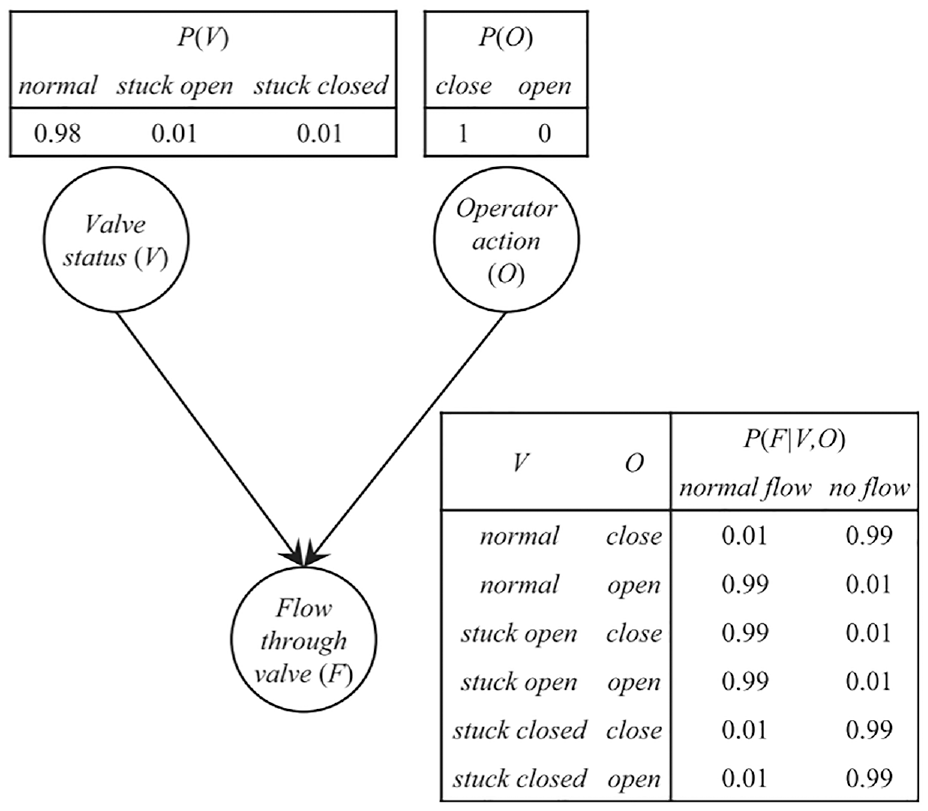
A Bayesian network graph of a simple system.²⁹

Figure 6.

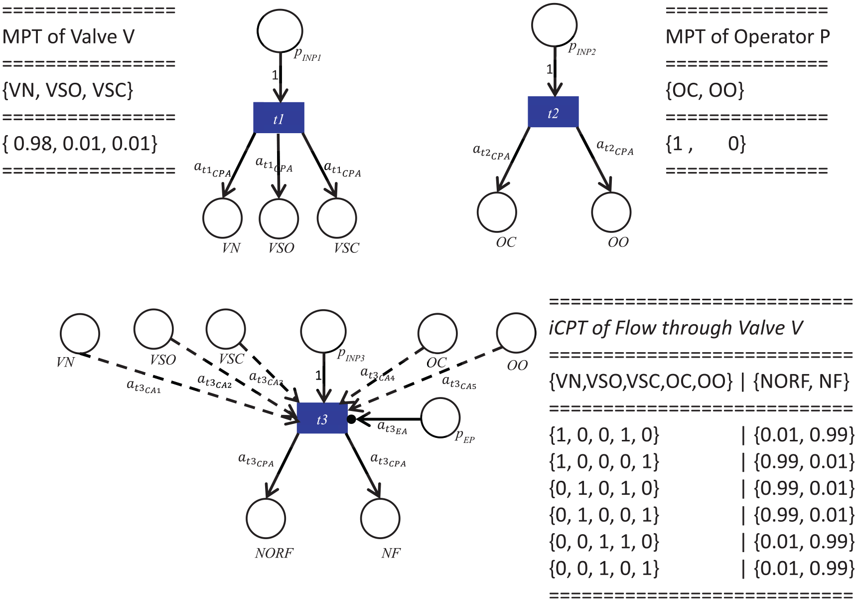
mBSPN model of the BN graph in Figure 5.

When a fault occurs in the system, places $p_{INP 1}$ , $p_{INP 2}$ and $p_{INP 3}$ will be marked with a token each, enabling the transitions $t 1$ , $t 2$ and $t 3$ in the mBSPN module of the GSPN-mBSPN approach. The level of dependency between system components and process variables determines the firing order of these transitions. To assign priorities to the transitions, the example study involves one level of dependency, where the states of V and O influence the state of F (Figure 5). Consequently, transitions t1 and t2 in Figure 6 have an equal, higher priority than transition t3. During transition enabling and firing check, either $t 1$ and $t 2$ will be randomly selected for firing. At this stage, the algorithm proceeds with the procedure Transition_Fire(), which involves invoking an inference sampling algorithm based on the chosen inference code at the beginning of the simulation of a GSPN-mBSPN model. For example, the procedure Compute_Rejection_ Sampling_One() is called for the case when the inference algorithm code is 2: rejection sampling. Within Compute_Rejection_Sampling_One(), the function Get_Sample_One() is utilised to generate a sample state for a component or process variable using the Marginal Probability Table (MPT) of the component or the input Conditional Probabilistic Transition (iCPT) of the process variable. The function Get_CPT_Row() is called inside Get_Sample_One() to select a probability row entry required for sampling the index of a conditional probabilistic place (CPP) in the vector of the CPP places of a CPT transition that will get a token when the transition is fired. In Get_CPT_Row(), the vector container for storing the current marking of the causal places of a CPT transition is first emptied. Then, if the transition is not independent, the markings of its causal places are stored in the vector container. However, since both t1 and t2 are independent conditional probabilistic transitions, the containers for their causal place markings remain empty. The probability row entry selected from the MPTs of t1 and t2 corresponds to the probability attribution of the CPP associated with the states of the components modelled by the CPT transitions. The next step involves generating a random number $r$ from a uniform distribution $U (0, 1)$ comparing it iteratively with the firing probability of the CPT transition (selected from its MPT or iCPT) to determine the current index of the CPP that will get a token after firing. For example, if the current index for t1 is 0, a token will be added to place VN. Similarly, if the current index for t2 is 1, the Conditional Probabilistic Place OO of t2 will receive a token upon firing.

Subsequently, Compute_Rejection_Sampling_One() checks if the firing CPT transition has evidence using the function Has_Evidence(). If it is an observable CPT transition, evidence is set for it based on its evidence place, $p_{EP}$ current marking. Then, the previously determined current index and evidence values of the CPT transition are compared. Inconsistency between the sampled index using the input and the observed real evidence leads to setting the firetest variable to false and returned. Then, Transition_Fire() is continued and a token is removed from the input place of the CPT transition. A token is also deposited in one of its CPPs depending on firetest value. If firetest is false, no CPP gets a token. If firetest is true, a CPP at index ‘current index’ gets a token. Every CPT transition is expected to deposit a token in one of its CPPs when it fires. But in rejection sampling, this depends on the firetest value. If firetest is false for a CPT transition, the sample is lost for that time instant and the CPT transitions are reanalysed at another observation time point. In the case study example, suppose t1 and t2 fire successfully with current indexes 0 and 1 at an observation time $τ$ . Then, the causal places marking t3 will be ${VN, VSO, VSC; OC, OO} = {1, 0, 0, 0, 1}$ . The probability row for this marking t3’s iCPT is ${0.99, 0.01}$ . This probability row is used in the function Get_CPT_Row() to determine the ‘current index’ for for the firing operation of t3.

Steps 3 and 4: Monte Carlo simulation analysis and results of a GSPN-mBSPN model

A GSPN-mBSPN model can be analysed using Monte Carlo simulation (MCS). Several simulation runs are needed to evaluate some performance metrics of a GSPN-mBSPN simulation model. During each simulation run, the marking of places and the number of times transitions fired in the model are recorded at each timestep. These recorded values are used to calculate performance metrics such as average failure, reliability and posterior probabilities of components at each timestep over the entire simulation runs. Figure 7 depicts a flowchart for performing a number of time steps MCS simulation analysis on a GSPN-mBSPN integrated model proposed in this paper. The embedded functions tagged A, B and C are self-contained processes during the simulation. However, due to the space limitation, the flowcharts of these processes are omitted in this paper. The flowchart for the time steps MCS analysis of a GSPN-mBSPN model can be implemented in a programming language such as C++, which is adopted in this paper.

Figure 7.

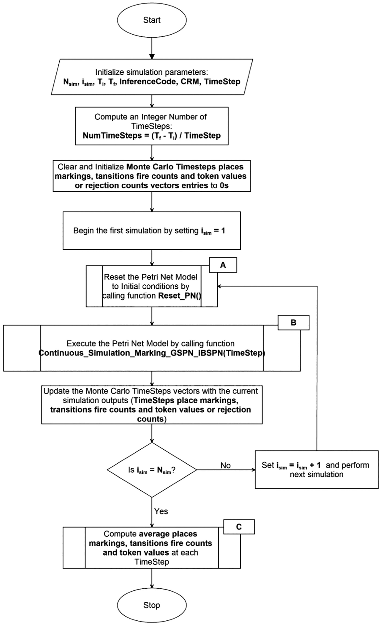
Flowchart of the Monte Carlo simulation analysis of a GSPN-mBSPN model application of the proposed methodology.

Application of the Proposed Methodology

The system description

Figure 8 shows a diagram of a simple water tank level control system for testing the methodology proposed in Section 2 of this paper. This system was taken from the work of Hurdle et al.³⁰ To diagnose the water tank system for any abnormality, the faults that could occur for each of the components of the water tank system need to be defined. Thus, Table 2 depicts a list of the system components’ possible states, including their failure states/modes. The water tank system can operate in either of two modes: active or dormant. In the active mode, considered in this paper valve V2 in the system is opened manually to draw water from the tank, and valve V1 is opened by controller C1 to replenish water in the tank if the water level detected by sensor S1 falls below the required level and closed if the required level has been reached. On the other hand, valve V3 can only open automatically by controller C2 if a critical water level that can cause overflow is detected in the tank by sensor S2. A further detailed description of this system can be found in the published articles by Hurdle et al. ³⁰ and Lampis and Andrews.³¹

Figure 8.

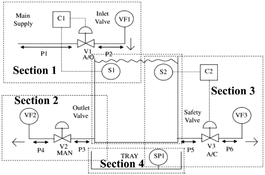
Schematic diagram of the water tank level control system.³⁰

Table 2.

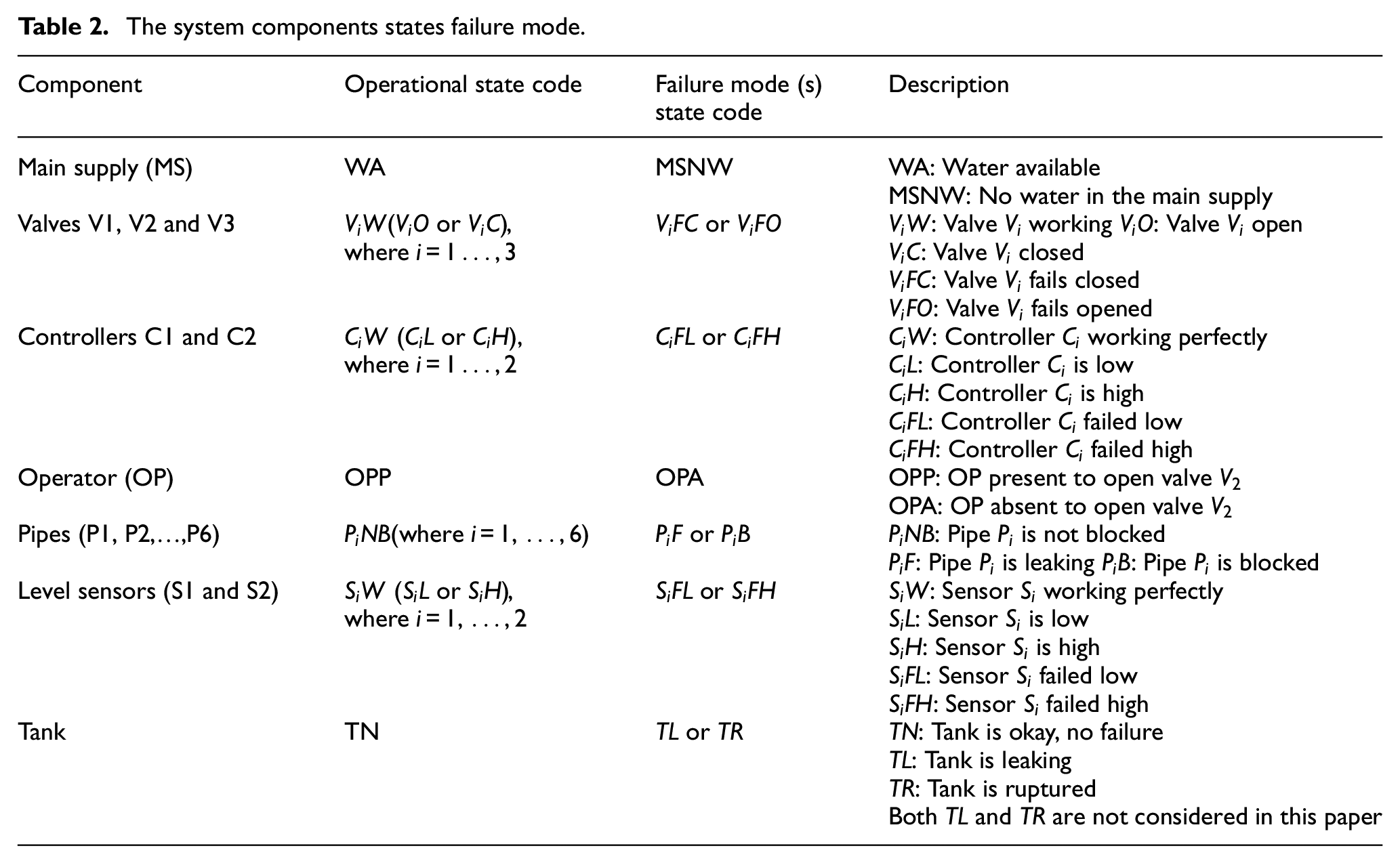
The system components states failure mode.

Component	Operational state code	Failure mode (s)state code	Description
Main supply (MS)	WA	MSNW	WA: Water available MSNW: No water in the main supply
Valves V1, V2 and V3	$V_{i} W (V_{i} O$ or $V_{i} C)$ ,where $i = 1 \dots, 3$	$V_{i} FC$ or $V_{i} FO$	$V_{i} W$ : Valve $V_{i}$ working $V_{i} O$ : Valve $V_{i}$ open $V_{i} C$ : Valve $V_{i}$ closed $V_{i} FC$ : Valve $V_{i}$ fails closed $V_{i} FO$ : Valve $V_{i}$ fails opened
Controllers C1 and C2	$C_{i} W (C_{i} L$ or $C_{i} H$ ),where $i = 1 \dots, 2$	$C_{i} FL$ or $C_{i} FH$	$C_{i} W$ : Controller $C_{i}$ working perfectly $C_{i} L$ : Controller $C_{i}$ is low $C_{i} H$ : Controller $C_{i}$ is high $C_{i} FL$ : Controller $C_{i}$ failed low $C_{i} FH$ : Controller $C_{i}$ failed high
Operator (OP)	OPP	OPA	OPP: OP present to open valve $V_{2}$ OPA: OP absent to open valve $V_{2}$
Pipes (P1, P2,…,P6)	$P_{i} NB$ (where $i = 1, \dots, 6)$	$P_{i} F$ or $P_{i} B$	$P_{i} NB$ : Pipe $P_{i}$ is not blocked $P_{i} F$ : Pipe $P_{i}$ is leaking $P_{i} B$ : Pipe $P_{i}$ is blocked
Level sensors (S1 and S2)	$S_{i} W (S_{i} L$ or $S_{i} H)$ ,where $i = 1, \dots, 2$	$S_{i} FL$ or $S_{i} FH$	$S_{i} W$ : Sensor $S_{i}$ working perfectly $S_{i} L$ : Sensor $S_{i}$ is low $S_{i} H$ : Sensor $S_{i}$ is high $S_{i} FL$ : Sensor $S_{i}$ failed low $S_{i} FH$ : Sensor $S_{i}$ failed high
Tank	TN	$TL$ or $TR$	$TN$ : Tank is okay, no failure $TL$ : Tank is leaking $TR$ : Tank is ruptured Both TL and TR are not considered in this paper

Developing the GSPN module of a GSPN-mBSPN model of a dynamic system

A GSPN-mBSPN model of a dynamic system, in this case the water tank level control system, is created based on the type of the modelling elements (places and transitions) and the arcs connecting them. Timed transition(s) with input and output places of type ‘component’ and without test/inhibitor places form a system component GSPN module. Besides, immediate transitions with common input and output places of type ‘component’ and test/inhibitor places of type ‘normal’ form a GSPN module for a system monitoring parameter. However, immediate transitions having common input and output places of type ‘component’ and test/inhibitor places equivalent to the input and output places of a lower-level GSPN module form an interconnection GSPN module for the propagation of a process variable. The input and output places of a GSPN module represent either the states of a component, monitoring parameter or propagated variable in the GSPN-mBSPN model of the water tank system. An incremental hierarchical approach was used to build the whole GSPN-mBSPN model. However, due to the mutual inter-dependencies between GSPN modules of the component, system monitoring parameter and propagated variables, the Petri net models were drawn using the following pattern filled notations for shared places similar to the colour-coded notations for shared places used by Boussif and Ghazel.³² The subsequent section describes the GSPN modules developed for the various components and subsystems of the water tank level control system.

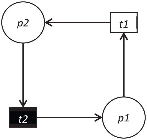
The system operating mode Petri Net model

The Petri net module for the operating mode of the water tank system is depicted in Figure 9 and represents part of the initial conditions required before a simulation can begin. A token in place p1 means the presence of an operator attempting to manually opens valve V2 to demand water from the tank. Thus, the system changes from the dormant state (place p2) to the active state (place p3). Conversely, if no operator is present to demand water from the tank (no token in place p1), the system switches from the active to the dormant state.

Figure 9.

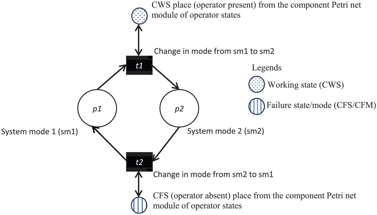
The system operating mode Petri net module.

The component Petri Net model

Following the system modelling steps discussed in step 2 of section 2, Figure 10 depicts the Petri net model for the working and failure state/modes of the types of the system components with single (e.g. pipes) and multiple (e.g. sensors, controllers and valves) failure states. Using the generalised Component Petri net model constructions depicted in Figure 10, the Petri net models for the modelled components of the water tank system including the states of an operator comprises of 37 component state/mode places and 22 failure state/mode transitions. For example, in Figure 10(b), a token in place p_w means a component is in a normal operational working state and the movement of the token from place p_w to p_fm1 when transition t_ttf fired after time ttf1 signifies the change in the component state from working to failure mode 1 state. At the beginning of the system operation, it is assumed that all components are working properly with the valves V1, V2 and V3 in closed states and the other components in their normal working states. In addition, constant failure times are assumed for all the components.

Figure 10.

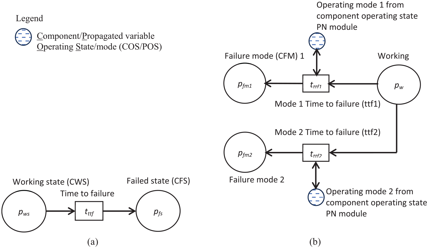
Petri net models for single (a) and multiple (b) operational states components.

The process variable (water level) state changes PN

In this paper, discrete places are used to represent the states/condition of the modelling entities, and the operation of the water tank level control system consists of both discrete (component states) and continuous (process variable states) variables. Thus, there is a need to develop a Petri net model to represent the continuous process variable states in discrete forms based on the operational reading of the level sensors monitoring the system process variable (water level in the tank). Figure 11 shows a generalised Petri net structure for the system process variable state changes. One token in the place ‘Tank portion with water’ represents a unit volume of water in a tank. One token in the tank level air place ‘Tank portion filled with air’ represents a free space of unit volume in a tank not occupied by water. Places p1 to pn correspond to the discretised states of a system process variable. The switching between the states of a system process variable is represented by the transitions t1–tn, and are governed by the weights (a1–an) of the test arcs between the places ‘Tank portion with water’ and ‘Tank portion filled with air’, and the transitions t1–tn. To construct the Petri net model for the system tank level states, the following assumptions were made:

i. The height of the tank is assumed to be equal to 2 m, and its cross-sectional area equal to 3.1415 m².

ii. It is assumed that the flow rate in section 1 is the same as the flow rate in section 2 of the system, but the flow rate in section 3 is twice the flow rate in section 1. The flow rate in section 1 is assumed to be Q = 0.006283 m³/s.

iii. It is assumed that overflow starts when the water level in the tank rises above 95 % of the tank level (i.e. >95% of 2 m = >1.9 m).

iv. The initial water level in the tank is assumed to be in the normal range and equals 80 % of the tank level (i.e. 80% of 2 m = 1.6 m).

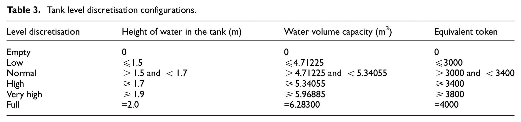
v. The level of water in the tank is discretised as empty (TLE), low (TLL), normal (TLN), high (TLH), very high (TLVH) and full (TLF).

vi. It is assumed that at every time step of 0.25 s, the increase or decrease in the tank level or volume is equal to 0.0005 m or 0.00157075 m³, which in turn is equivalent to 1 token increase or decrease in the number of tokens in a particular tank level place. Thus, for the tank level state discretisation Petri net model, the following configurations depicted in Table 3 were used to increase and decrease the water level in the tank.

Figure 11.

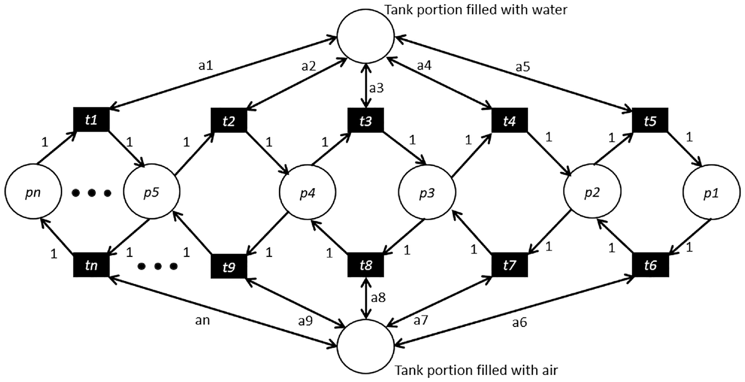
The generalised Petri net structure for the system process variable state changes.

Table 3.

Tank level discretisation configurations.

Level discretisation	Height of water in the tank (m)	Water volume capacity (m³)	Equivalent token
Empty	0	0	0
Low	≤1.5	≤4.71225	≤3000
Normal	>1.5 and <1.7	>4.71225 and <5.34055	>3000 and <3400
High	≥1.7	≥5.34055	≥3400
Very high	≥1.9	≥5.96885	≥3800
Full	=2.0	=6.28300	=4000

Using the generalised Petri net structure for the system process variable state changes depicted in Figure 11, the Petri net module for the water level state changes of the water tank system comprises of eight places (two auxiliary places for the system process variable states and six tank level discretised states places) and ten transitions for switching between tank level discretised states.

The operational states changes PN

The operational states changes models are developed by considering the working or failure modes of a component and the states of the inputs (e.g. the states of the immediate upstream components or process variable status change) connected to the component. Figures from 12 to 14 show the generalised Petri net modules for the operational states changes of a level sensor, controller and valve in the water tank system. The PN modules in Figure 12 are developed by considering the state of the water level in the tank and the working or failure modes of the sensor monitoring the water level. The presence of a token in either place p1, p2 or p3 and in the two shared places at the left-side in Figure 12 means a sensor (e.g. S1) has not failed and reads the water level inside the tank corresponding to the observed actual tank level state. In case of the failure of a level sensor (e.g. S1 failed low, S1FL), the sensor will ignore the true level of water in the tank and produces a reading corresponding to the current failure mode of the sensor as depicted by the Petri net structure at the right-side in Figure 12.

Figure 12.

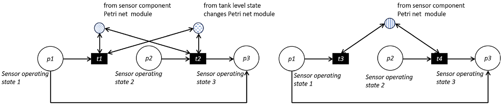
Working and failure operational state change PN models of a sensor.

A token in either place p1 or p2 in Figure 13 means a controller (e.g. C1) is sending a command signal (open or close depending on the operating state of the sensor and the state of the controller) to a valve (e.g. V1). In case of controller failure (e.g. C1 failed high, C1FH), the controller will ignore the actual command and send a spurious command to the valve based on the failure mode of the controller as depicted by the Petri net structure at the right-side in Figure 13. Likewise, a token in either place p1 or p2 in Figure 14 means a valve (e.g. V1) is in an operating mode (e.g. open or close depending on the operating signal command received from the controller and the current mode of the valve. If the valve has failed (e.g. V1 failed close, V1FC), the valve will ignore the controller’s actual command, and the valve will spuriously switch from the current operating mode to another or remain in the current mode depending on the occurred failure mode (i.e. firing of either transition t3 or t4 in Figure 14). The Petri net model for the remaining level sensor (S2), controller (C2) and valves (V2 and V3) in the water tank system has similar Petri net structures depicted in Figures 12 to 14, respectively. Thus, they are omitted from this paper. However, based on the generalised PN structure depicted in Figures 12 to 14, the Petri net models for the operational state changes of the sensors, controllers and valves in the water tank system comprise of 16 operating state places and 40 operating state change transitions.

Figure 13.

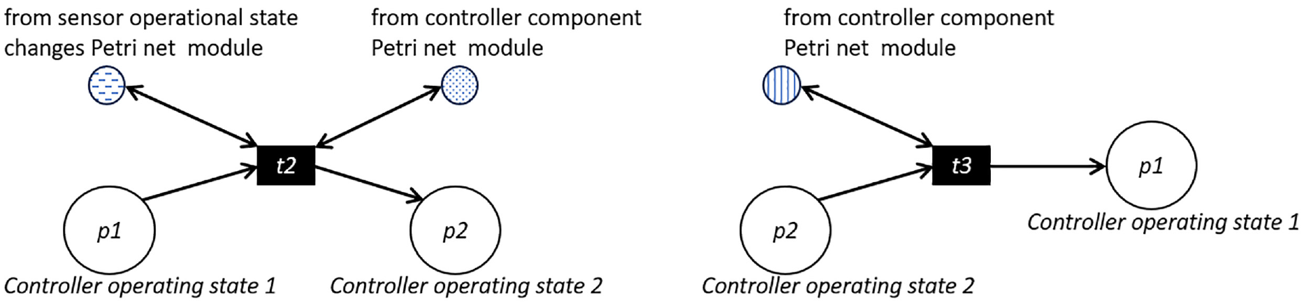
Working and failure operational state change PN models of a controller.

Figure 14.

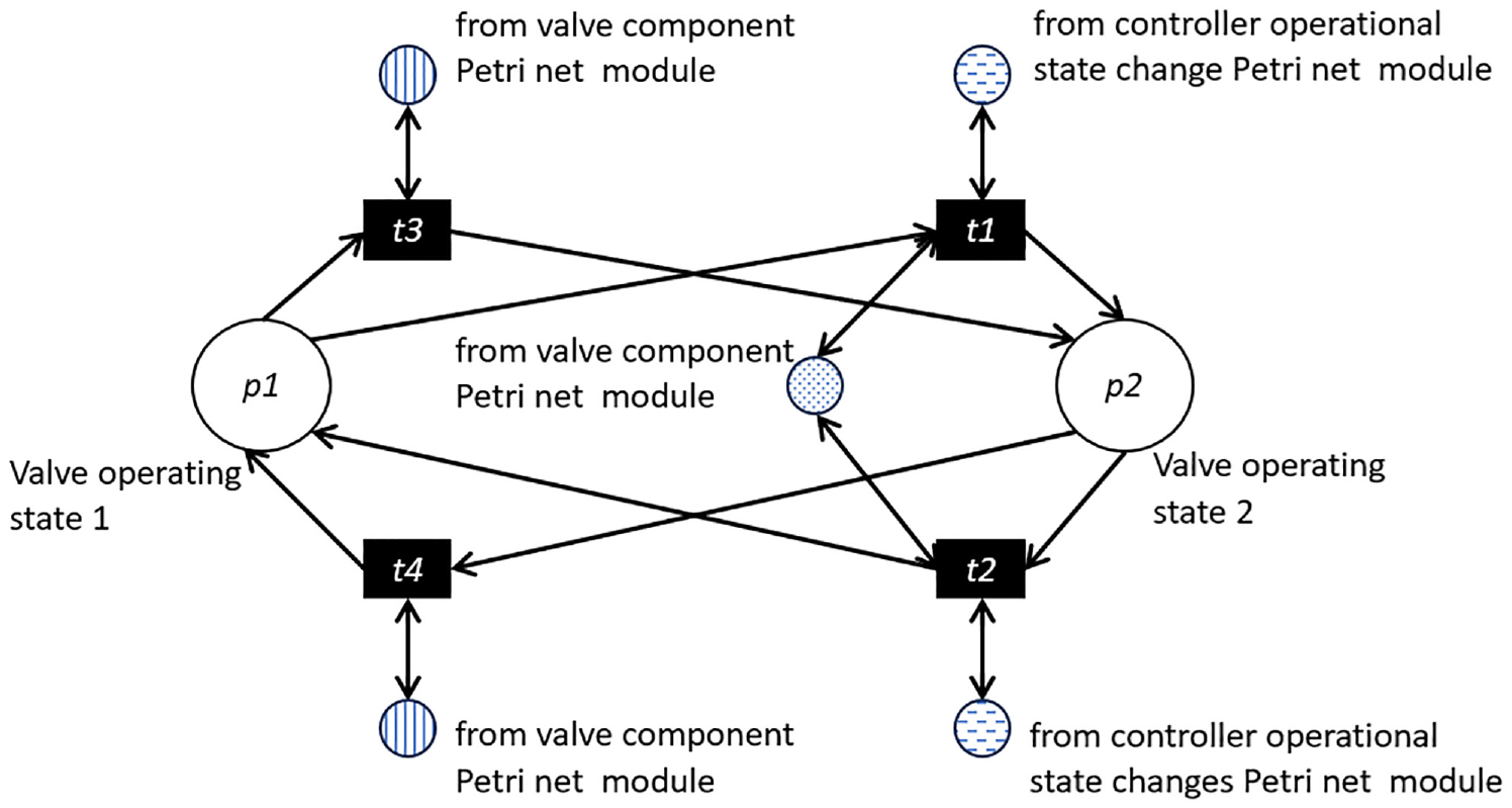
Working and failure operational state change PN model of a valve.

The flow propagation PN

Figure 15 shows the generalised PN structure for flow propagation, for example, inflow of water through one of the flow propagation components (i.e. pipelines P1) in section 1 of the water tank system. The model is developed by considering the working and the failure states of the component and the component states/operational modes of the immediate upstream component(s) connected to the component. In this case, places are created to represent all possible states of the material flowing through the component (e.g. flow or no flow of water). Besides, immediate transitions are created for switching between these places depending on the state of the component and/or the state/mode of the immediate upstream components connected to each of the immediate transitions. For example, in Figure 15, the shared place representing state of a current component (e.g. pipe P1) and the shared place for denoting the state of the immediate upstream component (e.g. water in the main supply) connected to the current component are connected to transition t1. A token in each of the shared places and place p1 will enable transition t1. Thus, when t1 is fired, the status of the current component will change from propagation variable state 1 (e.g. no flow) to state 2 (e.g. flow, place p2). The same Petri net structure in Figure 15 and the explained procedure is employed for the flow of process variable (water) through the remaining pipes and valves in the water tank system. Considering the generalised PN structure depicted in Figure 15, the Petri net models for the flow propagation in the water tank system comprises of 18 flow state places and 27 flow states changes transitions describing flows in the input and output flow sections of the water tank system.

Figure 15.

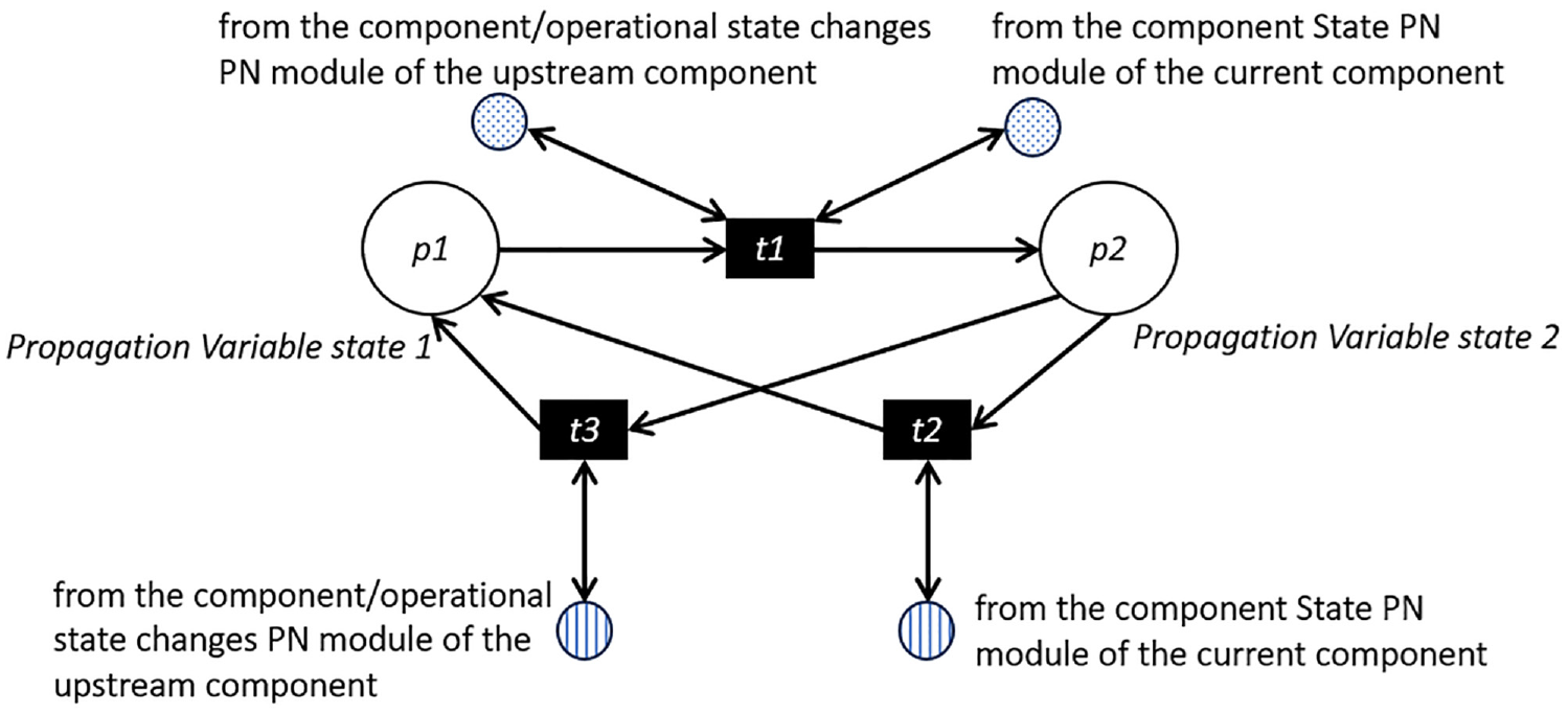
The flow propagation PN model at a section of a system.

Petri Net models for a system process variable (e.g. tank level) state updating and the section 4 (overspill tray) of the water tank system

The first three Petri net modules in Figure 16 depict generalised PN models of flow of a process variable (e.g. water) into a monitored process system (e.g. flow of water into the tank through the inlet pipe P2: the test place to transition t1 when transition t2 fired) or out of the system through the auxiliary downstream flow propagation components (e.g. flow of water out of the tank through the normal outlet pipe P4: the test place to transition t3 and the safety outlet pipe P6: the test place to transition t5 when transitions t4 and t7 fired, respectively) connected to flow control components (e.g. valves V1, V2 and V3 ). Transition t6 in the third Petri net module in Figure 16 will fire if there is still at least one token in the place p2 and there is no more process variable left in the process system to flow out of the safety out-flow section of the system. The first three Petri net models in Figure 16 are constructed such that the expected amount of a process variable to flow in and out of a monitored process system at each time step is first determined (token(s) in places p1, p2 and p3) based on the cross-sectional areas of the inlet and the auxiliary outlet flow propagation components. For the considered case study system, a unit of water (1 token) based on the water flow rate (0.00157075 m³/0.25 s) flows into or out of the tank depending on whether there is free space in the tank (at least one token in place ‘Tank portion filled with air’ from the system process variable state changes PN module) or water is left in the tank (at least a token in place ‘Tank portion with water’ from the system process variable state changes PN module). However, if deterministic transitions t1, t3 and t5 do not fire at the current time step, it means there is no possibility of water flowing via the auxiliary flow propagation components (i.e. in-flow via pipe P2, and out-flows via pipes P4 and P6).

Figure 16.

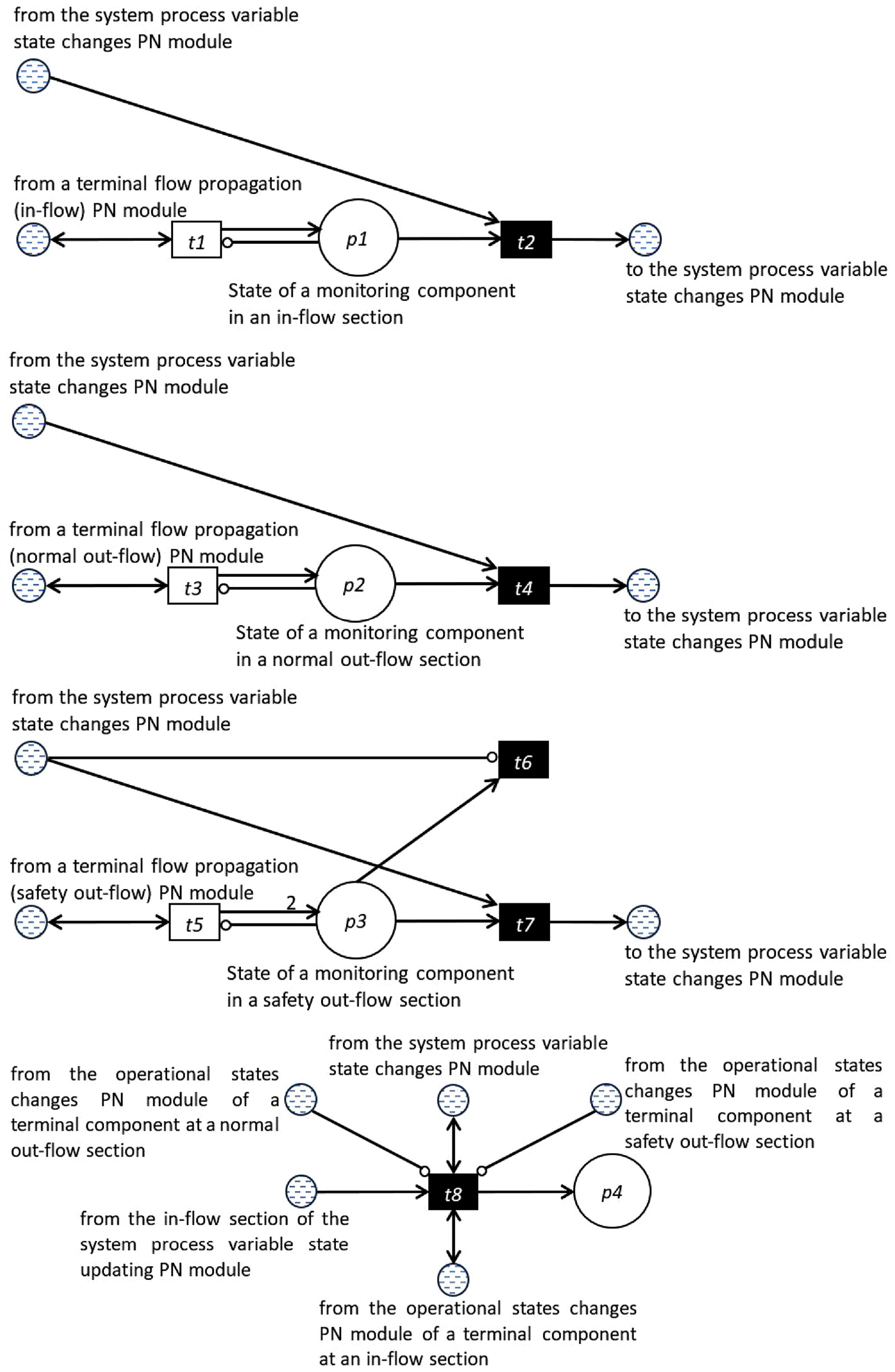
PN models for the process variable state updating and overspill tray.

The Petri net model at the bottom right of Figure 16 models the presence of water in the overspill tray as a result of a fault which resulted in an overflow. The transition t8 will fire if a process variable is not leaving the monitored process system through the auxiliary out-lets flow propagation components (e.g. no out-flow via pipes P4 and P5 of the water tank system when no token is present in both the flow states shared places from the operational state changes PN modules of pipes P4 and P5), and the shared place ‘state of a monitoring component in an in-flow section’ from the system process variable state updating PN model has a token while the system is already filled-up with a process variable (i.e. a token in a shared place from the system process variable state changes PN model denoting the full state of the process system). Thus, firing of transition t8 implies that an overflow has occurred, and place p4 will store the level of the spilled process variable (e.g. water) contained in the tray underneath the tank. With the given generalised PN modules depicted in Figure 16, the Petri net models for the system process variable (tank level) state updating and the section 4 (overspill tray) of the water tank system comprises of four places (three monitoring water flow state places, and one monitoring overspilled water level place), and eight transitions (three deterministic transitions for possible flow rates computation, three immediate transitions for tank level state updating, one auxiliary immediate transition and one immediate transition for the occurrence of overflow).

Sensor readings observation and fault detection Petri Net models

The Petri net module for the observation operation is used to reveal the actual condition of sensor reading outcomes at each section of the system. To continuously monitor failures in the system, the sensor readings observation Petri net modules are executed at every time step. Figure 17 shows an example Petri net structure for the observation operation. The time step observation is carried out using the loop p1-t1-p2-t2. Transition t1 is a deterministic transition with an observation time interval equal to the time step (0.25 s). Following the development of the sensor reading observation PN model, the fault detection PN models for the states of the observable monitoring components (flow and level sensors) in the system are developed using the generalised PN structure in Figure 3 which was described in sub-section formal definition of the GSPN-mBSPN approach in section 2. In summary, the fault detection Petri net modules for the water tank system comprises of 4 evidence places, 36 conditional output places and 12 conditional reset transitions (6 each for the system active and dormant operational modes).

Figure 17.

The sensor observation PN model.

The developed modified BSPN fault diagnostic PN model of the water tank system

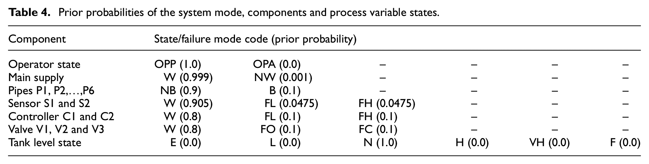
The first part of the proposed GSPN-mBSPN fault detection and diagnostic Petri net methodology for a dynamic system entails the development of the system’s behavioural model (i.e. the GSPN module of the GSPN-mBSPN approach). This has been presented in the first sub-section of this section for a simple case study (water tank level control system). The second part of the method involves the development of the fault diagnostic model (i.e. the mBSPN module of the GSPN-mBSPN approach) for the case study system. The mBSPN model is used to obtain the most likely components responsible for the observed faults/abnormalities in the operation of the system. All the transitions in the developed mBSPN module are conditional probabilistic transitions (CPTs) developed using the generalised structures of the different types of CPT transitions described in Figure 4 under the sub-section formal definition of the GSPN-mBSPN approach in section 2. The parameters for characterising the CPT transitions in the mBSPN module depend on the types of the CPT transitions. The independent CPTs are characterised by the prior failure probabilities of the states of system components. On the other hand, the parameters for describing the dependent non-observable and observable CPTs are the input conditional probability tables (iCPTs). The prior failure probabilities of the independent CPTs in all the system sections are depicted in Table 4. The iCPTs for the dependent non-observable and observable CPTs are determined based on the logic gates (AND, OR and NOT) representing the dependency structures of the system operational model. As stated in section 2 of this paper, the firing rules of the CPT transitions are governed by the selected approximate inference algorithms before the model simulation. The total number of conditional probabilistic places and CPT transitions in the developed mBSPN module of the water tank system are 85 and 36, respectively.

Table 4.

Prior probabilities of the system mode, components and process variable states.

Component	State/failure mode code (prior probability)
Operator state	OPP (1.0)	OPA (0.0)	–	–	–	–
Main supply	W (0.999)	NW (0.001)	–	–	–	–
Pipes P1, P2,…,P6	NB (0.9)	B (0.1)	–	–	–	–
Sensor S1 and S2	W (0.905)	FL (0.0475)	FH (0.0475)	–	–	–
Controller C1 and C2	W (0.8)	FL (0.1)	FH (0.1)	–	–	–
Valve V1, V2 and V3	W (0.8)	FO (0.1)	FC (0.1)	–	–	–
Tank level state	E (0.0)	L (0.0)	N (1.0)	H (0.0)	VH (0.0)	F (0.0)

System simulation and fault diagnostic analysis of the water tank system

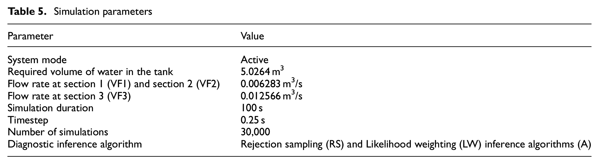
To assess the correctness and validity of the GSPN-mBSPN model of the water tank system, which aims to facilitate condition monitoring and enable early detection and diagnosis of single and multiple component failures, a custom C++ Monte Carlo Simulation (MCS) programme was created. The GSPN module of the GSPN-mBSPN model simulates system behaviour during normal operation and operation during the considered fault scenarios. Based on the description of the water tank system’s normal behaviour, the simulation results obtained (water level and flow rates) demonstrate the correctness of the GSPN-mBSPN model of the water tank system and validate the effectiveness of the developed programme in modelling and simulating a GSPN-mBSPN model of a dynamic system similar to the one described in this paper. The diagnostic accuracy of the GSPN-mBSPN approach will be assessed by comparing its results with those obtained from the HUGIN software³³ when applied to the water tank system model. The mBSPN module of the GSPN-mBSPN model of the water tank system diagnoses the cause of the faults using the sensor readings (evidence) from the GSPN simulation model describing the system operation. Therefore, the effects that the component faults would have on the system process variable (water level) and the input-and-output variables (flow) were observed by simulating the operation of the water tank level control system under single and multiple component failure scenarios using the simulation input parameters depicted in Table 5. The fault scenarios were investigated when the system was in the active mode of operation.

Table 5.

Simulation parameters

Parameter	Value
System mode	Active
Required volume of water in the tank	5.0264 m³
Flow rate at section 1 (VF1) and section 2 (VF2)	0.006283 m³/s
Flow rate at section 3 (VF3)	0.012566 m³/s
Simulation duration	100 s
Timestep	0.25 s
Number of simulations	30,000
Diagnostic inference algorithm	Rejection sampling (RS) and Likelihood weighting (LW) inference algorithms (A)

Simulation and diagnostic results of single component failure scenarios

One of the cases of single component failure scenarios is used to test the accuracy of the diagnostic results of the inference algorithms: rejection sampling (RSA) and likelihood weighting (LWA) inference algorithms implemented in this paper. As depicted in Figure 18, with the system in the ACTIVE mode and the initial volume of water inside the tank set to the normal required level, it is expected that starting from time t = 0.25 s, there should be flow (F) of water out of the tank in section 2, constant flow (CF) of water into the tank at section 1 and no water flow (NF) at section 3 of the system since the current level of water in the tank has not reached the safety level. Also, as shown in the figure, no water (NW) is inside the TRAY due to overflow, leaking or fracture and the level of water inside the tank remains constant from time t = 0.25–60 s.

Figure 18.

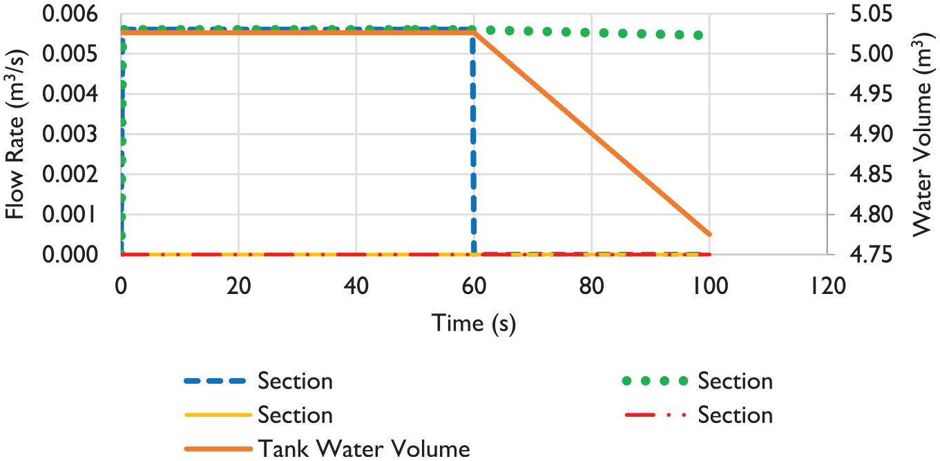
Flow and level sensors measurements when valve V1 failed closed at 60 s.

However, starting from time t = 60 s, the failure of one of the components in section 1 of the system, for example, valve V1 failed closed causes no flow in the section, as depicted in Figure 18. Consequently, this failure causes the volume of water in the tank to start decreasing at time t = 60 s since water is flowing out of the tank via valve V2 at section 2, and no more water is entering the tank through valve V1 at section 1.

To demonstrate the diagnostic capability of the implemented inference sampling algorithms, Figure 19 depicts the average posterior probabilities of the failure state/mode of the components in Section 1 of the water tank system that could be responsible for no flow at the section when valve V1 failed closed at t = 60 s using the LWA. Similar trends were observed for the RSA and thus omitted in this paper. The diagnostic results were generated with an average time of 3 min when the model was simulated 30,000 times on a Windows 10 64-bit Intel(R) Core (TM) i3 system with a 3.60 GHz processor and 8.00 GB of RAM. Running 30,000 simulations ensures the accuracy of the results presented in Figure 19 within ±5% precision and 95% confidence interval (CI) levels, as indicated by the convergence graph in Figure 20 for the posterior probability of no water in the main supply, being the component with the lowest failure probability (0.001). The 95% CI for the average posterior probability of no water in the main supply is in the interval [0.0017, 0.0019]. As shown in Figure 19, the posterior probabilities of blockage in pipes P1 and P2, valve V1 failed closed and controller C1 failed high are significantly higher than the posterior probabilities of the remaining components in the section. The presence of valve V1 failed closed among the list of the possible causes of no flow in section 1 of the system shows that the proposed methodology is accurate and could be used to diagnose single component failures with known observable effects on the system process variable (water level).

Figure 19.

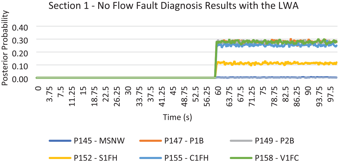
Timestep posterior probability of section 1 components failure state/modes with the no flow observation via section 1 of the system.

Figure 20.

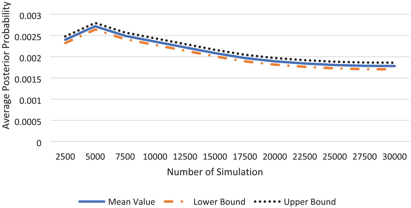
The posterior probability of no water in the main supply over the 30,000 simulations.

Table 6 summarises the results of the posterior probabilities of all the single component failure scenarios tested using LWA. Similar results are also obtained for the case of fault diagnosis with the RSA algorithm but are not presented due to brevity. As depicted in the table, it could be observed that single component failure scenarios whose effects correlate to the expected sensor symptoms at the sections of the system are hidden. Some of these failures could only be revealed if the component failure causes the level of water inside the tank to fall below or rise above the predefined low, high or very high set points (i.e. <1.5, >1.7 or >1.9 m), respectively.

Table 6.

Average posterior probabilities of single component failure scenarios based on failure diagnosis using likelihood weighting inference algorithm.

Section	Component	Inserted failure	Flow sensors observation	Probability		Successfully diagnosed?
Section	Component	Inserted failure	Flow sensors observation	Prior	Posterior	Successfully diagnosed?
1	Pipe P2	Blocked	No flow	0.1	0.1187	Yes
	Valve V1	Failed closed	No flow	0.1	0.1212	Yes
	Valve V1	Failed opened	Flow^a	0.1	–	No
	Pipe P1	Blocked	No flow	0.1	0.1204	Yes
	Controller C1	Failed high	No flow	0.1	0.0327	Yes
	Controller C1	Failed low	Flow^a	0.1	–	No
	Sensor S1	Failed high	No flow	0.0475	0.0486	Yes
	Sensor S1	Failed low	Flow^a	0.0475	–	No
	Main Supply MS	No water	No flow	0.001	0.0011	Yes
2	Pipe P4	Blocked	No flow	0.1	0.3694	Yes
	Pipe P3	Blocked	No flow	0.1	0.3701	Yes
	Valve V2	Failed closed	No flow	0.1	0.3657	Yes
	Valve V2	Failed opened	Flow^a	0.1	–	No
3	Valve V3	Failed opened	Flow	0.1	0.4472	Yes
	Valve V3	Failed closed	No flow^a	0.1	–	No
	Controller C2	Failed high	Flow	0.1	0.4173	Yes
	Controller C2	Failed low	No flow^a	0.1	–	No
	Sensor S2	Failed high	Flow	0.0475	0.1889	Yes
	Sensor S2	Failed low	No flow^a	0.0475	–	No
	Pipe P5	Blocked	No flow	0.1	–	No
	Pipe P6	Blocked	No flow	0.1	–	No

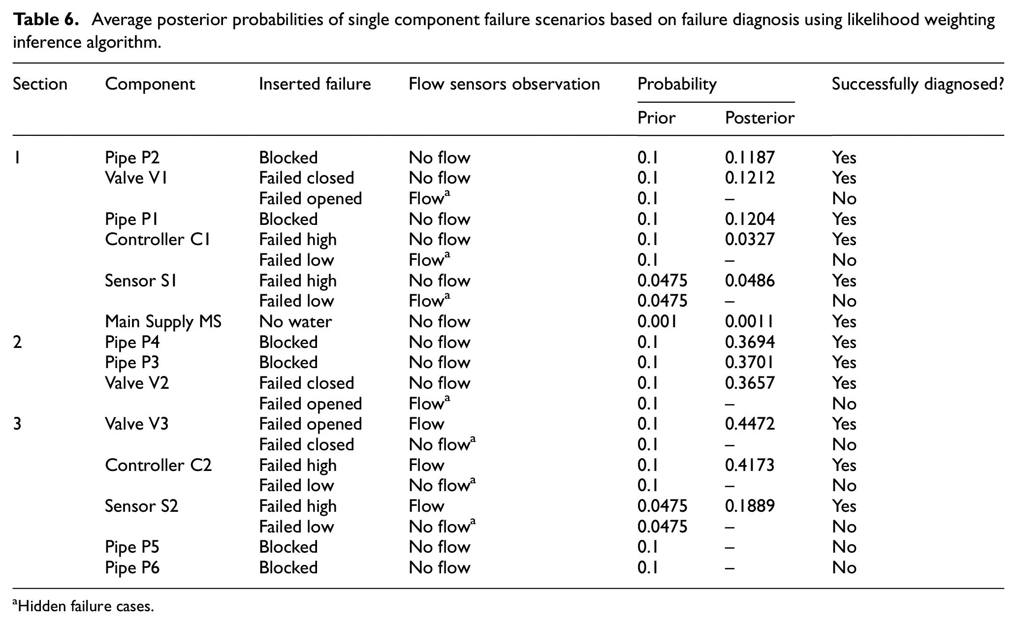
Hidden failure cases.

Note that in each case there were other components that had an increase in their posterior probability, but the failure that was inserted appeared at the top of that list, with the highest posterior probability.

Validation of the fault diagnostic capability of the GSPN-mBSPN model

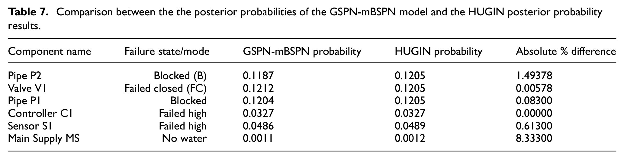
The fault diagnostic capability of the GSPN-mBSPN model was validated using a case involving the absence of flow through section 1 of the water tank system. The Bayesian network (BN) graph for the entire water tank system was drawn using the HUGIN software. However, only the BN graph for section 1 of the tank system is presented in Figure 21 for simplicity. To assess the effectiveness of the proposed GSPN-mBSPN method for fault diagnosis, evidence was applied to the ‘FV1_Status’ node in the BN graph, indicating a state of ‘no flow’ in section 1 of the tank system. The HUGIN software generated posterior probabilities (in percentage) for the states of the components in section 1, as revealed on the left-hand side of Figure 21. Although, as expected, there is an increase in the states of the posterior probability of the components that could be responsible for no flow in the section 1 of the water tank system. However, there are some differences in the posterior probabilities of the GSPN-mBSPN simulation output in Table 6 from the obtained results from the HUGIN software. This can be due to the precision and confidence interval issues of the Monte Carlo Simulation employed in the GSPN-mBSPN approach. However, the percentage difference is small, as shown in Table 7. Consequently, it can be concluded that the proposed GSPN-BSPN fault detection and diagnostic methodology is reliable, and its features hold promise for enhancing fault detection and diagnosis in complex systems.

Figure 21.

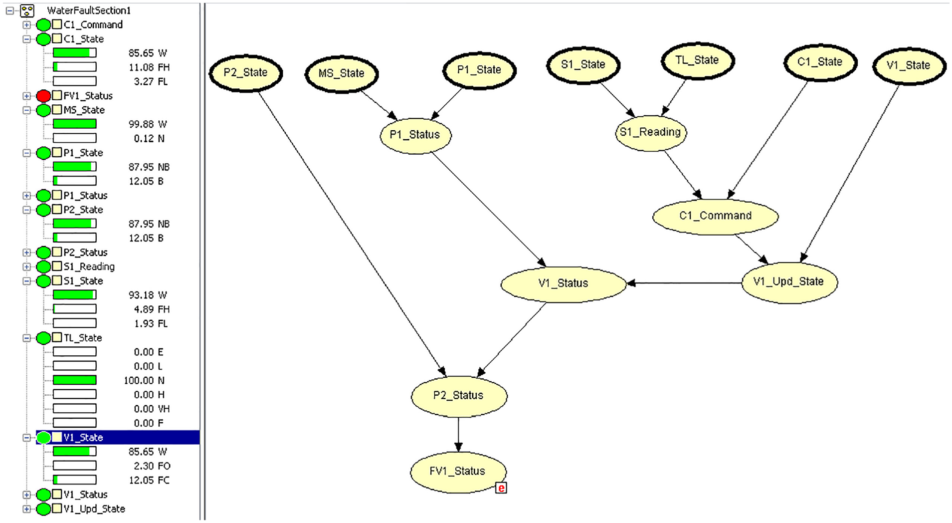
The Bayesian network graph of section 1 of the eater tank system.

Table 7.

Comparison between the the posterior probabilities of the GSPN-mBSPN model and the HUGIN posterior probability results.

Component name	Failure state/mode	GSPN-mBSPN probability	HUGIN probability	Absolute % difference
Pipe P2	Blocked (B)	0.1187	0.1205	1.49378
Valve V1	Failed closed (FC)	0.1212	0.1205	0.00578
Pipe P1	Blocked	0.1204	0.1205	0.08300
Controller C1	Failed high	0.0327	0.0327	0.00000
Sensor S1	Failed high	0.0486	0.0489	0.61300
Main Supply MS	No water	0.0011	0.0012	8.33300

Simulation and diagnostic results of multiple components failure scenarios

Several cases of multiple components failures in the water tank level control system were tested. However, to demonstrate the capability of the proposed methodology for multiple faults diagnosis, ten cases of multiple component failures (one component fault from Section 1, 2 and 3) that could cause continuous rise in the tank’s water level are taken as examples. Note, all faults occur at the same time. For illustration, Figure 22 shows the observed pattern of flow sensors rates and volume of water in the tank and overspill tray when sensor S1 failed low and valve V2 failed closed starting at time t = 60 s of the system operating time. The concurrent failure of sensor S1 (failed low) and valve V2 (failed closed) at t = 60 s causes continuous flow and flow stoppage at sections 1 and 2 of the system, respectively. This is evident from the observed flow patterns depicted in Figure 22. Consequently, as shown in the figure, these failures will cause the volume of water in the tank to start increasing at time t = 60 s since water is not flowing out of the tank via section 2 and there is a continuous supply of water into the tank at section 1 of the system.

Figure 22.

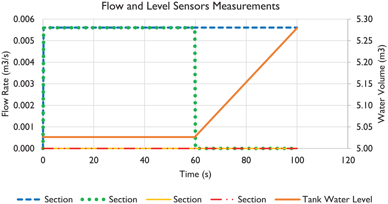
Flow and level sensors measurements when sensor S1 failed low and valve V2 failed closed at 60 s.

Table 8 summarises the results of the average posterior probabilities of ten cases of multiple components failure scenarios taking as examples to illustrate the capability of the proposed Petri net methodology for multiple faults diagnosis. Similar results are also obtained for the combination of other possible multiple failure scenarios but are omitted from this paper. As depicted in the tables, it could be observed that the average posterior probabilities of the components at Sections 1 and 2 of the tank system that could be responsible for the rise in the water level in the tank have increased.

Table 8.

Average posterior probabilities of multiple component failure scenarios based on failure diagnosis using likelihood weighting inference algorithm.

Case	Component	Inserted failure	Flow sensors observation	Probability		Successfully diagnosed?
Case	Component	Inserted failure	Flow sensors observation	Prior	Posterior	Successfully diagnosed?
1	Pipe P3	Blocked	No flow	0.1	0.3533	Yes
	Pipe P5	Blocked	No flow	0.1	0.0667	No
	Sensor S1	Failed low	Flow	0.0475	0.06	Yes
2	Pipe P3	Blocked	No flow	0.1	0.3280	Yes
	Sensor S1	Failed low	Flow	0.0475	0.0720	Yes
	Sensor S2	Failed low	No flow	0.0475	0.0160	No
3	Valve V2	Failed closed	No flow	0.1	0.3219	Yes
	Pipe P5	Blocked	No flow	0.1	0.1164	Yes
	Sensor S1	Failed low	Flow	0.0475	0.0616	Yes
4	Sensor S1	Failed low	Flow	0.0475	0.0647	Yes
	Pipe P4	Blocked	No flow	0.1	0.3453	Yes
	Pipe P5	Blocked	No flow	0.1	0.1511	Yes
5	Pipe P3	Blocked	No flow	0.1	0.2991	Yes
	Controller C1	Failed low	Flow	0.1	0.1251	Yes
	Pipe P5	Blocked	No flow	0.1	0.1022	Yes
6	Valve V2	Failed closed	No flow	0.1	0.4412	Yes
	Controller C1	Failed low	Flow	0.1	0.1471	Yes
	Pipe P5	Blocked	No flow	0.1	0.0588	No
7	Pipe P4	Blocked	No flow	0.1	0.3553	Yes
	Pipe P5	Blocked	No flow	0.1	0.1118	Yes
	Controller C1	Failed low	Flow	0.1	0.1053	Yes
8	Pipe P3	Blocked	No flow	0.1	0.2993	Yes
	Valve V1	Failed opened	Flow	0.1	0.1250	Yes
	Pipe P5	Blocked	No flow	0.1	0.1022	Yes
9	Valve V2	Failed closed	No flow	0.1	0.4012	Yes
	Valve V1	Failed opened	Flow	0.1	0.1250	Yes
	Pipe P5	Blocked	No flow	0.1	0.1111	Yes
10	Valve V2	Failed closed	No flow	0.1	0.3412	Yes
	Valve V1	Failed opened	Flow	0.1	0.1250	Yes
	Pipe P5	Blocked	No flow	0.1	0.0688	No

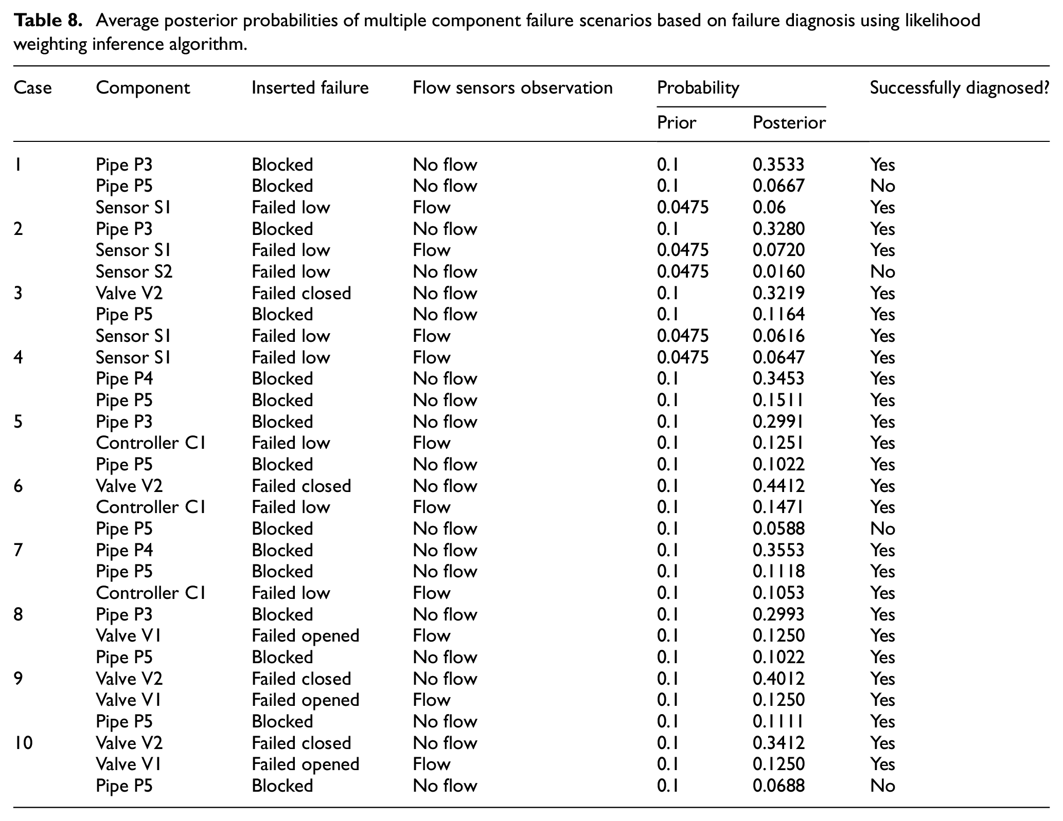
Besides, it was observed that there was not a lot significant difference between the prior and the posterior probabilities of the Section 3 components (Pipe P5 blocked) listed among the inserted faults in all the cases tested, excluding case 2, where the inserted fault from Section 3 is Sensor S2 failed low which also follow a similar pattern as in the other instances where pipe P1 is blocked. This is because this section only starts its functional operation if there has been a failure (s) that has caused the level of water in the tank to rise above the very high set-point which will occur from time t = 210 s based on the simulation input parameters assumed in this study. However, if any of the components in section 3 have failed, it is expected that the average posterior probabilities of the failed component (e.g. pipe P5 blocked in this case) will significantly increase. The little changes in the prior and the posterior probabilities of pipe P3 blocked in the example cases listed in Table 8 showed the capability of the proposed Petri net-based fault diagnostic methodology for computing marginal probabilities of system variables in a dynamic system with some unrevealed faults.

Conclusion

This paper proposes a condition monitoring, early fault detection and diagnostic Petri net methodology for diagnosing single and multiple faults in a dynamic system using a water tank level control system as a case study. The method was based on integrating Generalised and modified Bayesian Stochastic Petri Nets (GSPN-mBSPN) formalisms. First, a model describing the operational behaviour of the system was constructed using GSPN formalism. Then, a diagnostic model was constructed for the water tank system using a modified BSPN approach proposed in this paper. The GSPN and the mBSPN models were then integrated to aid real-time detection and diagnosis of faults in the system. This was achieved using newly proposed Petri net modelling features such as conditional reset and probabilistic transitions. The obtained posterior probabilities of the root causes of system failure scenarios showed the effectiveness and accuracy of using the proposed integrated Petri net methodology for single and multiple faults diagnosis in the considered water tank level control system. Due to the limited number of monitoring sensors and the points where they were deployed on the case study system, the proposed method fails to detect some cases of hidden faults. Thus, future research aims to improve the approach used for fault detection in the proposed methodology. Furthermore, additional component failures could also be considered, such as tank rupture and leakages at different tank levels. The methodology could be further enhanced by automatically generating the conditional probability tables required in the fault diagnostic model through the system simulation model.

Footnotes

Acknowledgements

The authors would like to thank Petroleum Technology Development Fund (PTDF), Abuja, Nigeria for funding and supporting Taofeeq Alabi Badmus PhD research through the fund Overseas Scholarship Scheme (OSS) programme [award number P6797054741222445].

Declaration of conflicting interests

The author(s) declared no potential conflicts of interest with respect to the research, authorship, and/or publication of this article.

Funding

The author(s) disclosed receipt of the following financial support for the research, authorship, and/or publication of this article: This work was supported by the Petroleum Technology Development Fund (PTDF), Abuja, Nigeria, under its PhD Overseas Scholarship Scheme award to Taofeeq Alabi Badmus [award number P6797054741222445].

ORCID iDs

Taofeeq Alabi Badmus

Rasa Remenyte-Prescott

References

Gao

Shardt

YAW

. Dynamic system modelling and process monitoring based on long-term dependency slow feature analysis. J Process Control 2021; 105: 27–47.

Bucelli

Paltrinieri

Landucci

. Integrated risk assessment for oil and gas installations in sensitive areas. Ocean Eng 2018; 150: 377–390.

Cai

Liu

Xie

. A real-time fault diagnosis methodology of complex systems using object-oriented Bayesian networks. Mech Syst Signal Process 2016; 80: 31–44.

Reeves

Remenyte-Prescott

Andrews

, et al. A sensor selection method using a performance metric for phased missions of aircraft fuel systems. Reliab Eng Syst Saf 2018; 180: 416–424.

Song

Salvo Rossi

Khan

, et al. Model-based information fusion investigation on fault isolation of subsea systems considering the interaction among subsystems and sensors. J Loss Prev Process Ind 2020; 67: 104267.

Wang

, et al. Recent advances in sensor fault diagnosis: a review. Sens Actuators A Phys 2020; 309: 111990.

Reeves

Remenyte-Prescott

Andrews

. Sensor selection for fault diagnostics using performance metric. Proc IMechE, Part O: J Risk and Reliability 2019; 233: 537–552.

Zhao

Cheng

. Sensor fault diagnosis based on adaptive arc fuzzy DBN-petri net. IEEE Access 2021; 9: 20305–20317.

Wootton

Andrews

Lloyd

, et al. Risk modelling of ageing nuclear reactor systems. Ann Nucl Energy 2022; 166: 108701.

10.

Lakehal

Nahal

Harouz

. Development and application of a decision making tool for fault diagnosis of turbocompressor based on Bayesian network and fault tree. Manag Prod Eng Rev 2019; 10: 16–24.

11.

Chiachío

Prescott

, et al. A new paradigm for uncertain knowledge representation by Plausible Petri nets. Inf Sci (N Y) 2018; 453: 323–345.

12.

Codetta-Raiteri

Portinale

. Approaching dynamic reliability with predictive and diagnostic purposes by exploiting dynamic Bayesian networks. Proc IMechE, Part O: J Risk and Reliability 2014; 228: 488–503.

13.

Weber

Medina-Oliva

Simon

, et al. Overview on Bayesian networks applications for dependability, risk analysis and maintenance areas. Eng Appl Artif Intell 2012; 25: 671–682.

14.

Chiachío

Prescott

, et al. Plausible Petri nets as self-adaptive expert systems: a tool for infrastructure asset monitoring. Comput-Aided Civ Inf Eng 2019; 34: 281–298.

15.

Taleb-Berrouane

Khan

Amyotte

. Bayesian Stochastic Petri Nets (BSPN) - A new modelling tool for dynamic safety and reliability analysis. Reliab Eng Syst Saf 2020; 193: 106587.

16.

Zhou

Reniers

. Probabilistic Petri-net addition enabling decision making depending on situational change: the case of emergency response to fuel tank farm fire. Reliab Eng Syst Saf 2020; 200: 106880.

17.

Codetta-Raiteri

Portinale

. Generalized continuous time Bayesian networks as a modelling and analysis formalism for dependable systems. Reliab Eng Syst Saf 2017; 167: 639–651.

18.

Kabir

Papadopoulos

. Applications of Bayesian networks and Petri nets in safety, reliability, and risk assessments: a review. Saf Sci 2019; 115: 154–175.

19.

Andrews

Fecarotti

. System design and maintenance modelling for safety in extended life operation. Reliab Eng Syst Saf 2017; 163: 95–108.

20.

Calvert

Neves

Andrews

, et al. Incorporating defect specific condition indicators in a bridge life cycle analysis. Eng Struct 2021; 246: 113003.

21.

Moradi

Groth

. Modernizing risk assessment: a systematic integration of PRA and PHM techniques. Reliab Eng Syst Saf 2020; 204: 107194.

22.

Bartlett

Hurdle

Kelly

. Integrated system fault diagnostics utilising digraph and fault tree-based approaches. Reliab Eng Syst Saf 2009; 94: 1107–1115.

23.

Remenyte-Prescott

Andrews

. Fault propagation modelling for fluid system health monitoring. Int J Performability Eng 2011; 7(2): 137–154.

24.

Balbo

. Introduction to generalized stochastic Petri nets. In: Bernardo

Hillston

(eds) Formal methods for performance evaluation. Berlin, Heidelberg: Springer, 2007, pp.83–131.

25.

Nourredine

Menouar

Campo

, et al. A new generalized stochastic Petri net modeling for energy-harvesting-wireless sensor network assessment. Int J Commun Syst 2023; 36: e5505.

26.

Andrews

Prescott

de Rozières

. A stochastic model for railway track asset management. Reliab Eng Syst Saf 2014; 130: 76–84.

27.

Andrews

. A modelling approach to railway track asset management. Proc IMechE, Part F: J Rail and Rapid Transit 2013; 227: 56–73.

28.

Russell

Norvig

. Artificial intelligence a modern approach. 3rd ed. Upper Saddle River, NJ: Pearson Education, Inc., 2010.

29.

Zhao

Tong

Zhang

. Rapid source term prediction in nuclear power plant accidents based on dynamic Bayesian networks and probabilistic risk assessment. Ann Nucl Energy 158; 2021: 108217.

30.

Hurdle

Bartlett

Andrews

. Fault diagnostics of dynamic system operation using a fault tree based method. Reliab Eng Syst Saf 2009; 94: 1371–1380.

31.

Lampis

Andrews

. Bayesian belief networks for system fault diagnostics. Qual Reliab Eng Int 2009; 25: 409–426.

32.

Boussif

Ghazel

. Model-based monitoring of a train passenger access system. IEEE Access 2018; 6: 41619–41632.

33.

HUGIN. HUGIN researcher version 8.0, https://www.hugin.com/hugin-developerhugin-researcher/ (2016, accessed July 19, 2023).

A novel fault detection and diagnostic Petri net methodology for dynamic systems

Abstract

Keywords

Introduction

Proposed methodology

Step 1: System description and analysis

Step 2: System operational and fault diagnostic PN module construction

Overview of the GSPN-mBSPN approach

Formal definition of the GSPN-mBSPN approach

Enableness and firing rules of transitions in the GSPN-mBSPN

Illustrative example of the fault diagnostic process of the GSPN-mBSPN methodology

Steps 3 and 4: Monte Carlo simulation analysis and results of a GSPN-mBSPN model

Application of the Proposed Methodology

The system description

Developing the GSPN module of a GSPN-mBSPN model of a dynamic system

The system operating mode Petri Net model

The component Petri Net model

The process variable (water level) state changes PN

The operational states changes PN

The flow propagation PN

Petri Net models for a system process variable (e.g. tank level) state updating and the section 4 (overspill tray) of the water tank system

Sensor readings observation and fault detection Petri Net models

The developed modified BSPN fault diagnostic PN model of the water tank system

System simulation and fault diagnostic analysis of the water tank system

Simulation and diagnostic results of single component failure scenarios

Validation of the fault diagnostic capability of the GSPN-mBSPN model

Simulation and diagnostic results of multiple components failure scenarios

Conclusion

Footnotes

Acknowledgements

Declaration of conflicting interests

Funding

ORCID iDs

References