
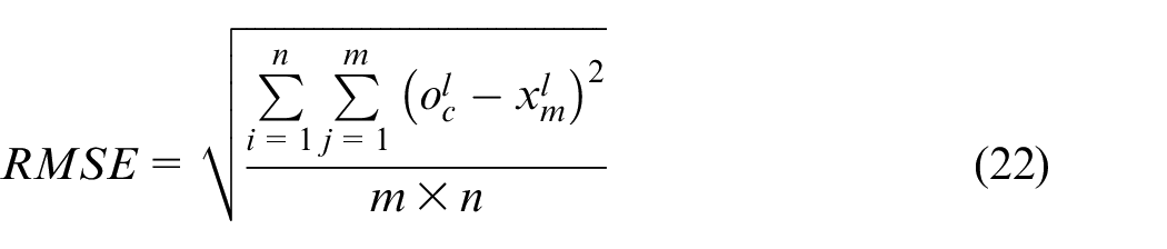
Abstract
To address the problems of the poor feature extraction ability and weak data generalization ability of traditional fault diagnosis methods in reciprocating shale gas compressor fault diagnosis applications, in this study, a fault diagnosis method for reciprocating shale gas was developed. This method uses a novel optimized learning method, free energy in persistent contrastive divergence, in deep belief network learning and training. It solves the problem of the deep belief network classification ability degradation in long-term training. The root mean square error is used as the fitness function to search for the optimal parameter combination of the DBN network by using the sparrow search algorithm. At the same time, the learning rate and batch size of the deep belief network, which have a large impact on the training error, are selected for optimization. Then, the original vibration signal is preprocessed by calculating 13 different time domain indicators, and feature-level data and decision-level data are fused in a parallel superposition method to obtain a fused time domain index dataset. Finally, combined with the powerful adaptive feature extraction and nonlinear mapping ability of deep learning, the constructed sample dataset is input to the deep belief network for training, and the deep belief network based on reciprocating shale gas compressor fault diagnosis model is established.
Keywords
Introduction
Mechanical equipment monitoring and fault diagnosis are widely used in the electric power, petrochemical, metallurgy, aviation, and other industries, and they have become the technical basis for modern equipment management and improving the overall benefits for enterprises. Reciprocating compressors are important equipment for ensuring the pressurization of shale gas. 1 Reciprocating compressors use shale gas as a medium for compression under high-pressure conditions. Failure of the reciprocating compressor can cause serious personal injury or death. Therefore, the study of fault diagnosis technology for reciprocating compressors, early detection of abnormal faults, and corresponding preventive measures can bring huge economic benefits to enterprises. 2
The fault diagnosis process of reciprocating shale gas compressor (RSGC) generally includes three steps: sensor-based status signal monitoring, signal feature extraction based on signal analysis methods, and data-driven methods. 3 Because the first two methods require a large amount of knowledge of the failure mechanism, it is impossible to diagnose this type of RSGC with massive failure data effectively. Therefore, because the data-driven fault diagnosis method of reciprocating compressors has stronger data processing ability than the other two methods, it has been studied frequently. 4 The quality of feature extraction directly affects the fault diagnosis of the RSGC.5–7 With the development of artificial intelligence, machine-learning-based fault diagnosis methods have become increasingly popular, such as artificial neural networks (ANNs),8–10 probabilistic neural networks, 11 and support vector machines (SVMs). 12 Tran 13 collected vibration acceleration, pressure, and current as fault diagnosis signals and used the Teager–Kaiser energy operator to estimate the envelope amplitude signal of the vibration signal and wavelet analysis to eliminate random noise in pressure and current signals. Then, the features were extracted from the preprocessed data. A well-trained network can effectively distinguish six valve states. Qin 14 used the basis tracking method to reduce the noise of the vibration signal of the valve cover, extracted the fault features from the signal by wave matching, and finally used the SVM to perform pattern recognition on the fault. Zhang 15 used the scatter matrix method to extract sensitive eigenvalues from the crosshead vibration signal and used an SVM to diagnose the fault of the reciprocating compressor. In the past 10 years, the above-mentioned feature extraction methods have been able to perform certain diagnoses on some key components of reciprocating compressors. Ma et al. 16 converted the original one-dimensional vibration signal from the time domain to the frequency domain using a Fourier transform. Then, the frequency domain signal was used as the input of a one-dimensional convolutional neural network (CNN), and the convolutional layer was used to achieve adaptive feature extraction. Finally, the network output layer used the softmax function to realize the pattern recognition of multiple failures. The above-mentioned shallow-learning-based methods showed good performance in failure mode classification. However, because the diagnostic accuracy of shallow learning largely depends on the quality of the extracted fault features, it not only requires a good understanding of the application field, but also requires considerable adjustment and time. In the fault detection of reciprocating compressors, shallow-learning methods have insufficient diagnostic capabilities, exposing the limitations of extracting appropriate features from fault signals with high similarity.
The structure of a RSGC is complicated. There are many vulnerable parts, the movement between the structures is relatively large, and the force of the structural parts is complicated. Therefore, the faults of RSGCs are diverse, the correlation between the faults is strong, and the complexity is high.17–19 This makes the manual diagnosis process more difficult, so the diagnosis process not sufficiently timely. The accuracy of the diagnosis results largely depends on the experience and knowledge of the diagnosis expert. Therefore, it is necessary to reduce manual participation in the diagnosis process and improve the diagnostic accuracy for RSGCs. In the past 60 years, the development of artificial intelligence has made great progress. Various types of artificial-intelligence technologies provide methods for solving complex nonlinear and large-scale engineering problems. 20
The deep belief network (DBN) is a classic algorithm in deep-learning theory. With its excellent feature extraction and training methods, it has successfully solved information retrieval, dimensionality reduction, speech recognition, fault classification,21–23 and other problems. First, DBN pretraining is an unsupervised-learning method that eliminates the dependence on labeled samples in the training process. At the same time, the DBN-based fault diagnosis method can reduce the uncertainty of the manual feature extraction method in the fault diagnosis process and extract effective fault features from the fault data. 24 Second, the DBN method has a wide range of adaptability and powerful mapping capabilities. It can approximate any continuous function, so it is often used to simulate multivariable nonlinear systems. Therefore, the DBN has become an established fault diagnosis tool.
Since the DBN network was proposed, much research has been conducted on the method of selecting the structure parameters of the DBN. The proposed methods include the incremental method, trial-and-error method, and genetic algorithm. Gustavo 25 proposed the introduction of the firefly algorithm into the calibration of the number of DBN hidden layers in binary image reconstruction, as well as the use of metaheuristics to fill the gaps in the optimization of DBN hidden-layer parameters. This method greatly improves the convergence speed and accuracy of parameter setting, but it has a high time complexity and sensitivity for parameter initialization.
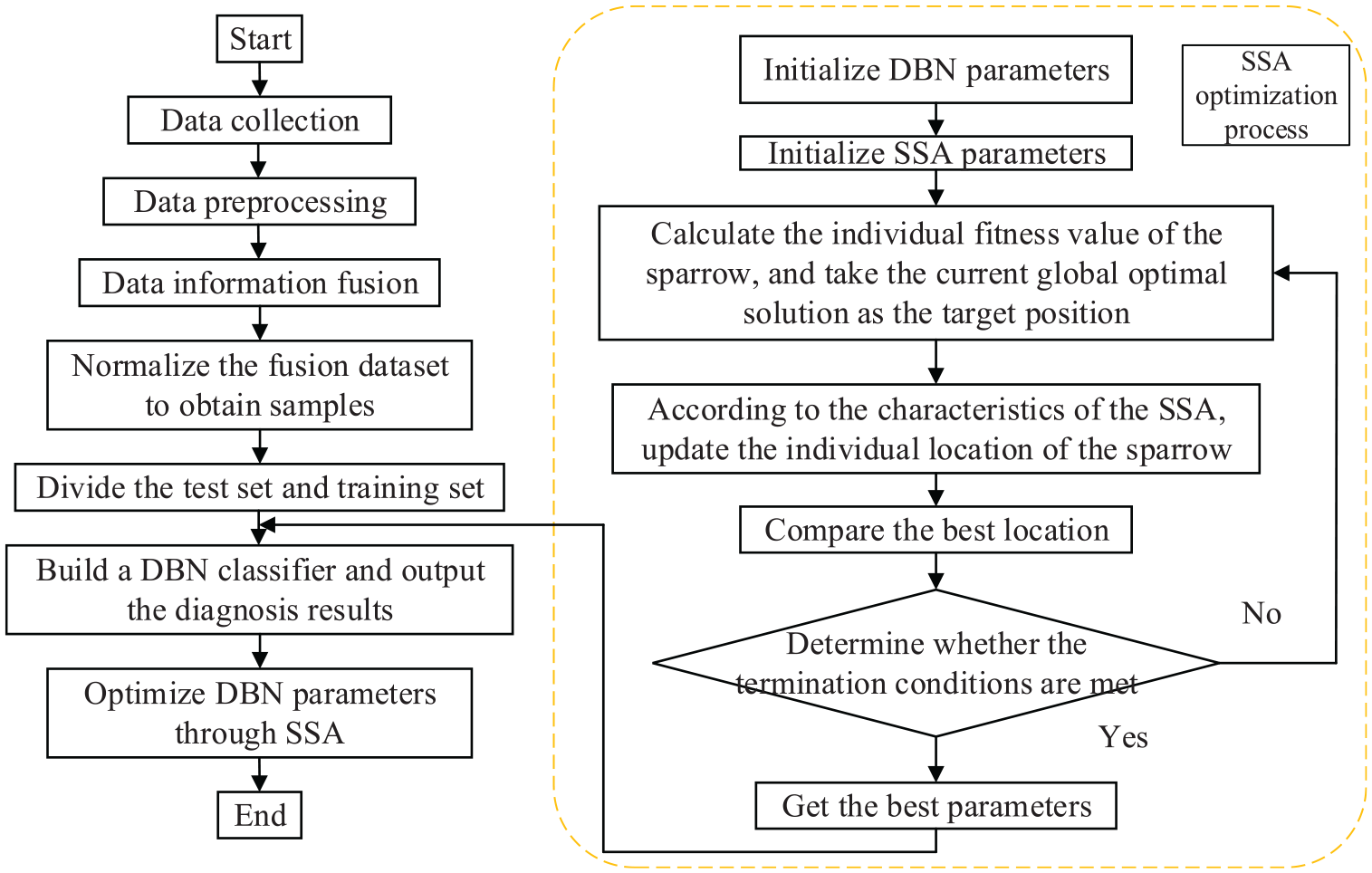
Currently, the selection of the DBN network structure and setting the learning rate and other hyperparameters have a significant impact on the classification results of DBN. However, the existing DBN algorithm mainly adjusts the above parameters based on prior knowledge to determine the DBN network model. In addition, it may fall into a local extremum during the optimization process, and the convergence speed is slow and inaccurate. Therefore, in this study, the sparrow search algorithm (SSA) with strong optimization ability and faster convergence speed was used to optimize the DBN network adaptively to solve these problems. The free energy in persistent contrastive divergence (FEPCD) method ensures that the network model obtains a better chain selection during sampling learning and improves the quality and efficiency of the gradient approximation in the DBN training process, thereby improving the classification ability of the model. In this method, the original vibration signal is preprocessed by calculating 13 different time domain indicators, and feature-level data and decision-level data are fused in a parallel superposition method to obtain a fused time-domain index dataset. Second, the improved structure parameters of the FEDBN are adaptively optimized through the SSA. Finally, the divided training set is input into the SSA-FEDBN model for pretraining, and an SSA-FEDBN-based fault diagnosis model for a RSGC is established. The experimental results show that the DBN fault diagnosis network optimized by SSA can effectively improve the classification accuracy of the DBN in RSGC fault diagnosis. The main contributions of the proposed method are summarized as follows.
(1) The proposed method uses the FEPCD method to ensure that the network model can obtain better chain selection during sampling and learning. It improves the quality and efficiency of the gradient approximation in the DBN training process, thereby improving the classification ability of the model.
(2) This method solves the general problems of weakness and complexity of fault features in reciprocating compressors by constructing a classification model that considers both multifeature fusion and deep learning.
(3) The proposed method incorporates the SSA for parameter optimization of the DBN, which is often a difficult task in DBN construction and has a crucial effect on model performance. Taking advantage of the superior exploration capability, search accuracy, and search efficiency of the SSA, the method can avoid human interference and uncertainty caused by the random selection of hyperparameters.
Deep belief network optimization algorithm
Deep belief network
The DBN is based on multiple restricted Boltzmann machines (RBMs). 26 Each RBM is divided into two parts: a visible and a hidden layer. 27 Each layer is independent of the other, and the layers are connected by connection weights. The data are passed between the layers through the sigmoid activation function according to the corresponding learning rules. The RBM network is stacked layer by layer according to this rule, as shown in Figure 1. Thus, it is a three-layer DBN model. The DBN learning process consists of pretraining and reverse supervised fine tuning. 28
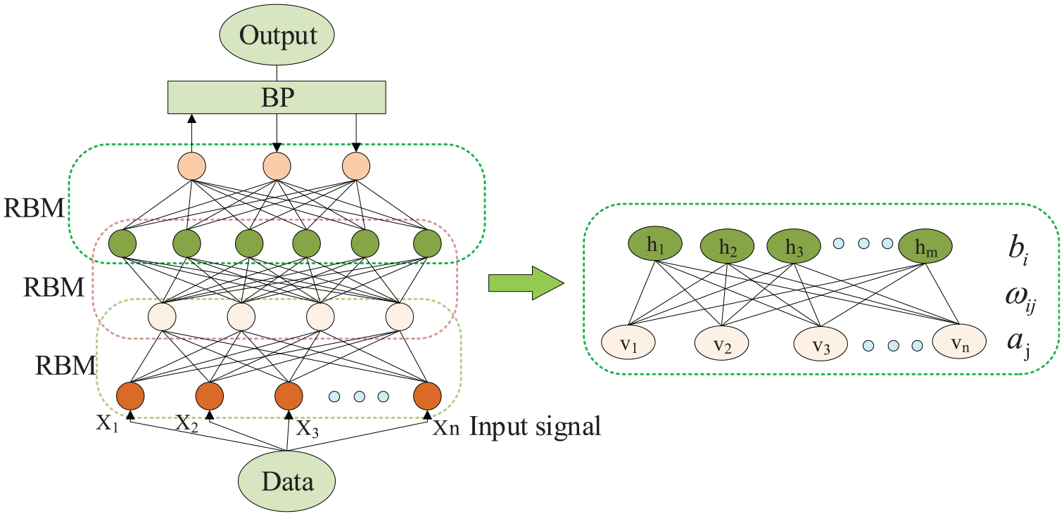
DBN basic structure.
Pretraining
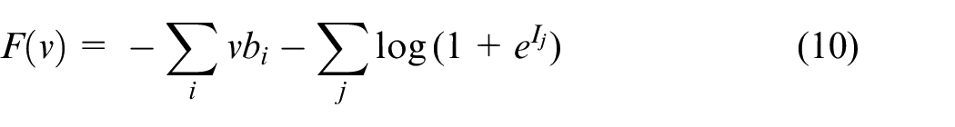
The RBM model is derived from the energy model of thermodynamics, and its network structure is derived from a neural network. Each layer of the model network consists of several neurons, and each neuron has only two states: activated and inactivated. The energy function formula is29,30
where
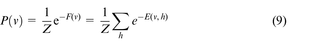
Its joint probability is
where
The activation function is derived as
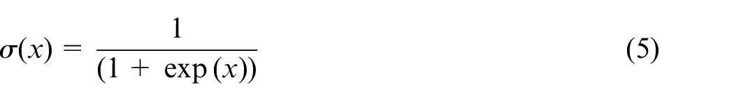
where
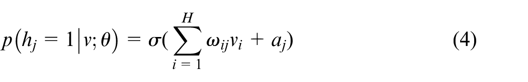
The maximum-likelihood function is used to maximize equation (4) and find the parameter
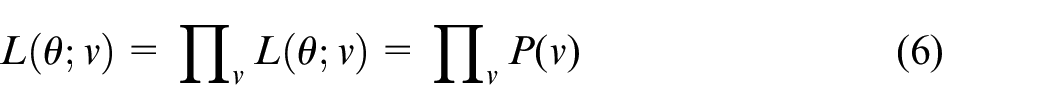
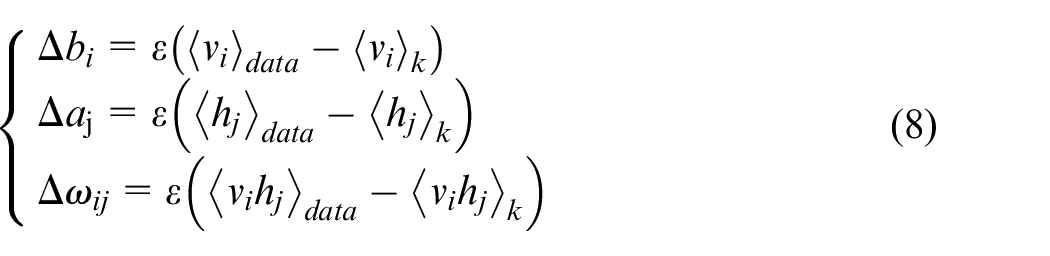
The maximum of the likelihood function is obtained by the random gradient rise method, and the partial derivative of the parameter
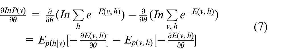
The first term in equation (7) refers to the probability of
Improved DBN algorithm
To solve the above problems, Hinton
31
proposed a contrast divergence (CD) sampling algorithm to learn RBMs quickly. The algorithm originated from Gibbs sampling. The visible layer is initialized with the training data, and the unit of the hidden layer is calculated using equation (4). After the state of the hidden layer is determined, the value of the visible layer is recalculated using equation (3), that is, the visible layer is reconstructed once. Therefore, the update criteria for the parameter
where
Although, the learning effect of the CD algorithm is better in the initial stage of training, as the learning process progresses and the network parameter values increase, its ability to approximate gradients decreases. Therefore, the persistent contrast divergence (PCD) algorithm was introduced for learning the DBN network. The PCD algorithm uses the state of the last chain in the previous update step and estimates it using a continuous Gibbs sampling run (unlike the CD method), which initializes the visible layer with training data. Although the model parameters change gradually with the number of iterations, they change very little. A small amount of Gibbs sampling can be used to obtain a good sample from the model distribution.
The FEPCD method used in this study is a PCD optimization method based on free energy. In the PCD method, many continuous chains can run in parallel. The choice of chain in this method is random and not necessarily the best. The quality of chain selection is related to the accuracy of sample training. The FEPCD method can ensure that the network model obtains a better chain selection when sampling learning and improves the quality and efficiency of the gradient approximation in the DBN training process to improve the classification ability of the model. Therefore, the FEPCD method utilizes the following selection criteria to obtain the best chain based on the free energy of the visible-layer sample.32,33
where
Fine tuning
After the forward learning is completed, the RBM initialization parameters of each layer are obtained, but these network parameters are not the optimal values, and the backward fine-tuning process must be adjusted according to the value of the error function. Reverse fine-tuning learning is a supervised-learning process, using the back propagation (BP) training algorithm to optimize the parameters of each level to find the optimal network structure value, so as to fit the target value more accurately. The reverse tuning algorithm selected in this study is the BP network algorithm, which remembers the input training set as
The BP algorithm only needs to locally search the parameters of the constructed network and optimize and adjust the network parameters according to the error function. It can efficiently learn and adjust the network.
Sparrow search algorithm
The sparrow foraging process can be abstracted as a finder–adder model, and a reconnaissance and early warning mechanism can be added. The finder itself is highly adaptable and has a wide search range, which guides the population to search and forage. 34 The sparrow collection matrix is expressed as

where
The fitness value matrix of the sparrow is expressed as


where
The finder movement rule mathematical expression is
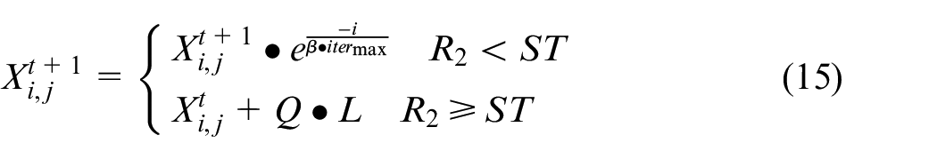
where
The follower movement rule mathematical expression is
Here,
As for the investigator behavior, when the population is looking for food, some sparrows are selected to be on guard. When an enemy approaches, both the finder and the follower give up the current food and fly to another location. Each generation randomly selects SP (generally 10%–20%) sparrows from the population for early-warning behavior.
The mathematical expression of investigator movement rules is
Here,
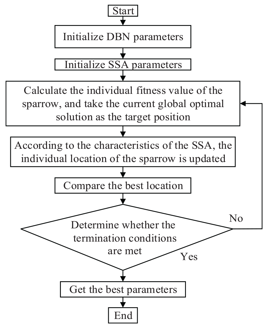
SSA optimizing the FEDBN process
The SSA can effectively achieve global optimization without being affected by initial parameter selection. Therefore, the SSA is used to optimize the FEDBN network structure adaptively. Figure 2 is the SSA-based FEDBN optimization algorithm flow chart.
SSA-based FEDBN optimization algorithm flow chart.
The optimization steps of the SSA on the FEDBN parameters are as follows.
Step 1: Initialize the FEDBN network parameters.
Step 2: Initialize the sparrow population parameters, set the number of finders in the population, and set the percentage of individuals who are found to be dangerous.
Step 3: Calculate the fitness values for the initial population, sorted from smallest to largest, and select the current best and worst values.
Step 4: Update the locations of the finder, follower, and investigator to determine the current global best location.
Step 5: If the current best position is better than the previous iteration, perform the update operation; otherwise, do not perform the update operation, and continue the iterative operation.
Step 6: If the loss of the training sample satisfies the discrimination condition or the number of iterations reaches the upper limit, the optimization ends, and the global optimal value and the best fitness value are obtained. The optimal parameters of the output network. Otherwise, return to step 3 and repeat steps 4 and 5 until the judgment conditions are met.
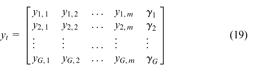
Multisensor data fusion
Time domain analysis
The health status characteristics of the RSGC can be judged by the time domain characteristic parameters. However, for different time domain parameters, the sensitivity and stability of the fault differ. Even for similar failures on different types of RSGC, there is no unified standard to judge the vibration of the key components of RSGCs. In this study, the SSA-FEDBN and information fusion technology were used to diagnose the fault of a RSGC.
After the vibration information of the RSGC was collected through sensors installed at different positions of the RSGC, 13 time-domain indicators are calculated to preprocess the original vibration signal. These include the root mean square value, variance value, peak value index, impulse index, kurtosis index, mean value, maximum value, minimum value, peak-to-peak value, square root amplitude, average amplitude, waveform index, and margin index.
Multisensor data fusion technology
The use of multisensor data fusion technology enables information from different time points and different sources to be fused semi-automatically or automatically. Through the optimal combination, more-effective information can be obtained. 35 The time domain statistical feature values reflecting the vibration intensity, combined with data- and feature-level fusion technology, are used to obtain a multisensor information fusion dataset. The specific process is as follows. Figure 3 is the flow chart of multisensor data fusion.
(1) Collect signals from different acceleration sensors:

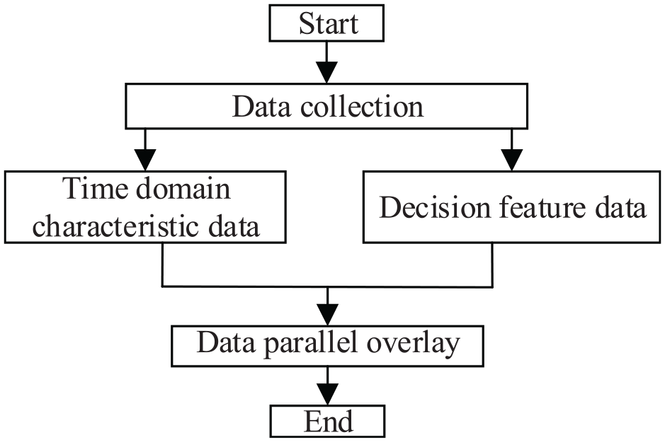
Flow chart of multisensor data fusion.
Here, n represents the number of sensors.
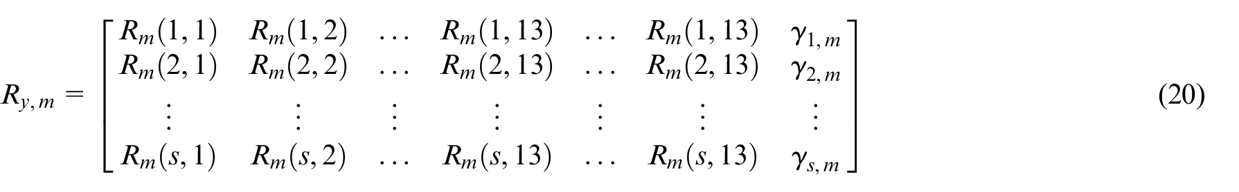
(2) For the collected multisource finite discrete sequence signal, the original fault information matrix is
where
(3) Calculate 13 important statistical characteristic values that reflect the vibration intensity.
(4) Based on the parallel superposition method, combining feature- and data-level fusion technology, multisensor information fusion data

Fault diagnosis model based on SSA-FEDBN
The specific flow of the fault diagnosis model based on SSA-FEDBN is as follows. Figure 4 is the flow chart of fault diagnosis model of RSGC based on SSA optimized FEDBN.
(1) Collect vibration signals through sensors installed on RSGCs and define fault classifications according to different faults.
(2) Obtain the fused dataset by calculating the time domain index of
(4) Normalize the fused data set. After the fused dataset is normalized, the preprocessed data sample is obtained, and the fault diagnosis model is tested or trained.
(5) Divide the data sample.
(6) Search for the best combination of structure parameters of the FEDBN network by SSA adaptation. The best structure distribution is obtained when the root mean square error (RMSE) trained in the FEDBN reaches the minimum.
Where,
Flow chart of fault diagnosis model of RSGC based on SSA optimized FEDBN.
(7) The SSA is used to optimize the FEDBN to obtain a fault diagnosis model, and datasets are input into the SSA-FEDBN model to output classification results.
Experimental
Data description and data preprocessing
When the piston moves from one end of the cylinder to the other end, the volume formed by the upper end surface of the cylinder and the cylinder head gradually increases. The gas pushes the valve plate in the air valve from the intake pipe to enter the cylinder. With the movement of the piston, the amount of gas entering the cylinder from the pipe increases and remains until the piston reaches the bottom dead center. When the piston starts to return from the bottom dead center, the intake valve automatically closes and no longer inhales. 36 When the pressure of the compressed gas increases to a certain value, the gas rushes through the exhaust valve and is output from the exhaust pipe until the piston reaches the top dead center. During this period, the gas pressure in the cylinder no longer increases.37,38 To verify the method, data were collected from RSGCs in the petroleum industry. Owing to its confidential commercial nature, relevant information about the RSGC cannot be provided, but the structure and sensor layout of the RSGC are shown in Figure 5. The functions of each sensor are listed in Table 1. The signal collected by the sensor reflects the operating status of the RSGC.
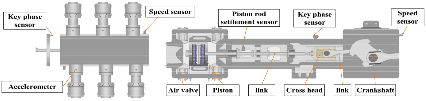
RSGC structure and sensor layout diagram.
Sensor type and function.
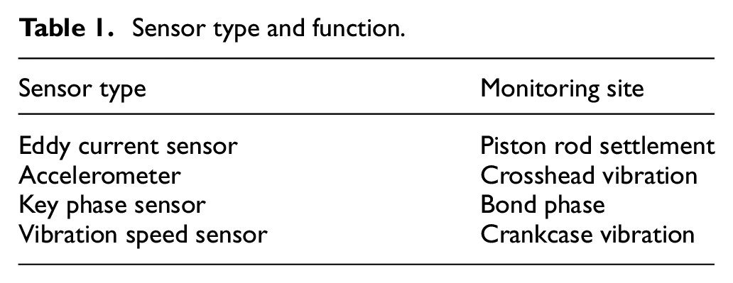
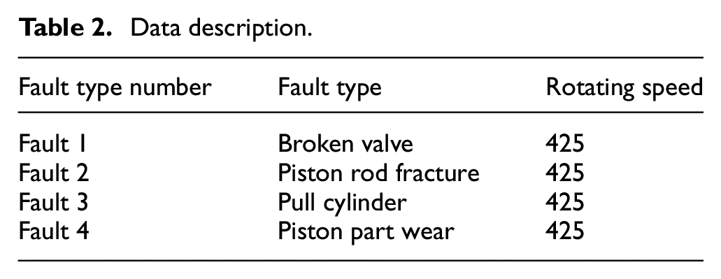
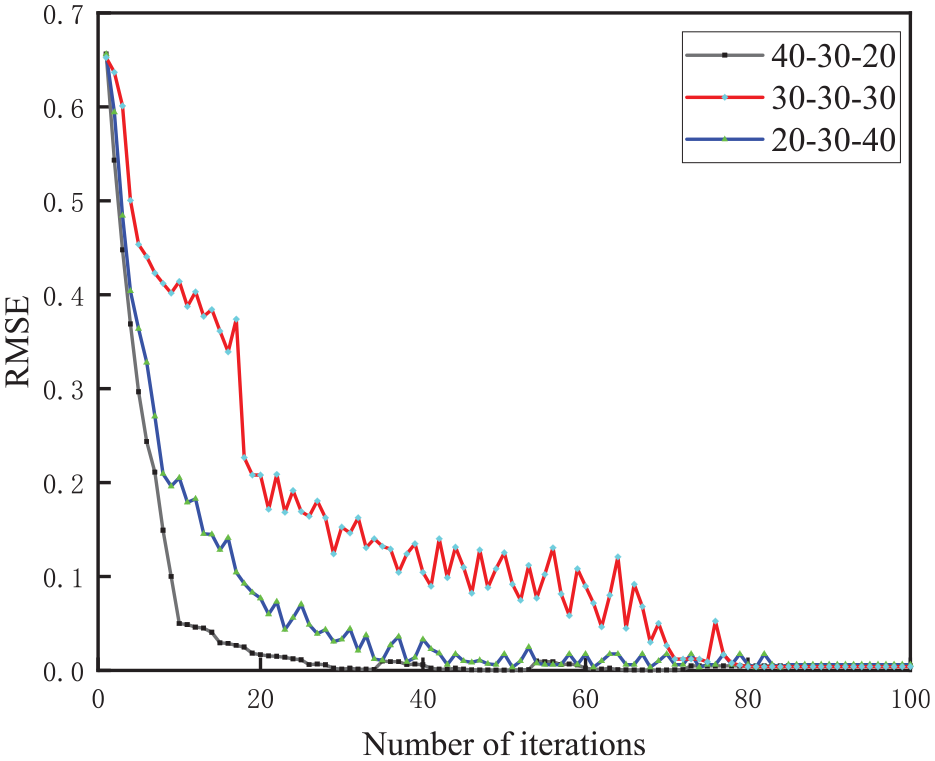
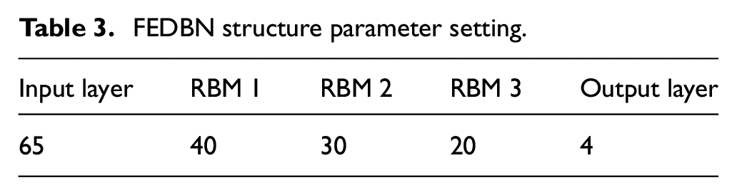
Figure 6 shows four typical failure images of RSGCs obtained from the factory. When the RSGC fails, the vibration is transmitted along a certain transmission path in the main body of the RSGC and measured by the cylinder accelerometer. The fault type information is shown in Table 2. A total of 10,091,520 vibration signals were collected at a speed of 425 rpm and a sampling frequency of 14.5 kHz, and the original signals were preprocessed using the proposed method. Combining feature index formula, 1024 line measurement units were used to calculate different time domain indicator characteristic parameters. Therefore, a 1971 × 66 fusion matrix was obtained, and 80% of the data in each group were randomly selected for training and 20% for testing to verify the SSA-FEDBN model.
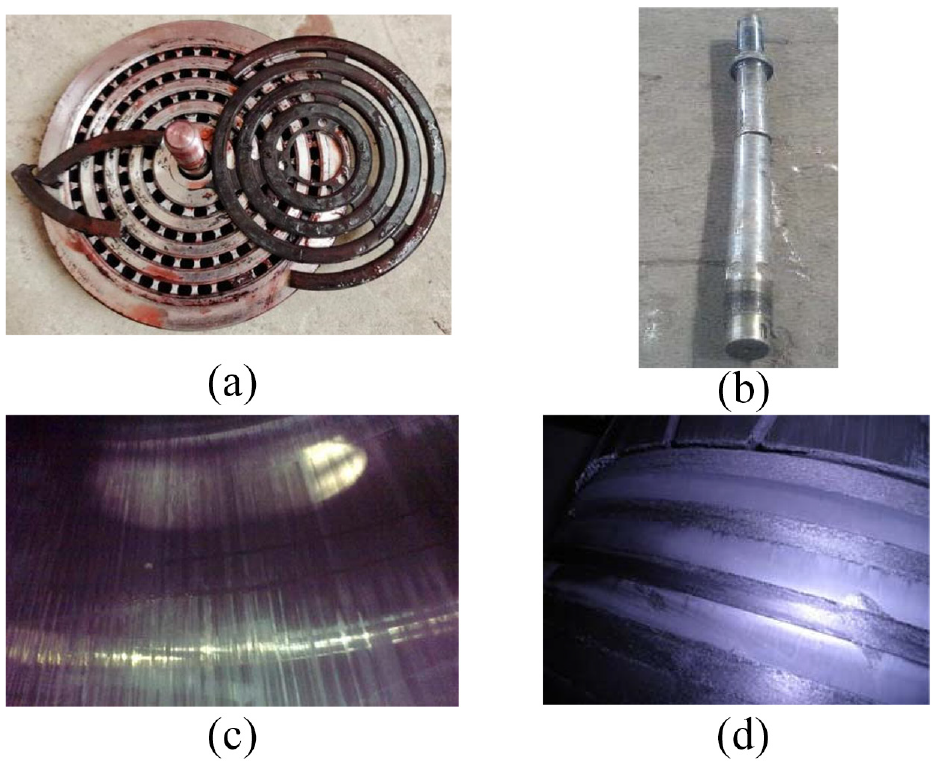
Four failures of RSGC: (a) broken valve, (b) piston rod fracture, (c) pull cylinder, and (d) piston part wear.
Data description.
FEDBN optimal parameter combination and determination of network structure
Because there is no prior knowledge to determine the number of hidden layers, in this study, the smoothing (30-30-30), increasing (20-30-40), and decreasing (40-30-20) hidden-layer structures were compared and analyzed. Finally, the optimal number of hidden layers was determined.
The SSA algorithm was first used to search adaptively for the optimal parameters of learning rate and batch size in a FEDBN network, with search ranges of [0.01,1] and [1,100]. In the SSA parameter setting, the number of finder sparrows and that of the sparrows aware of danger accounted for 20% and 10%, respectively, and the warning value was 0.8.
After the parameters of the SSA were set, an adaptive optimal parameter search was performed on the above three network structures. Figure 7 shows the relationship between the RMSE of the decreasing network (40-30-20) and the number of iterations. The RMSE of the decreasing network converges to approximately 0.001005 to reach the minimum value. After 34 calculations, the iterations start to converge. The results show that the SSA search algorithm has a strong global search ability and strong optimization ability, which are suitable for adaptively searching for FEDBN network structure parameters. Under the above conditions, the optimal parameter combination of the FEDBN network obtained by the decreasing type (40-30-20) is [0.1923,33]. The same operation was performed for the smoothed (30-30-30) and increasing (20-30-40) types, with results of [0.3578,35] and [0.6679,25], respectively.
Relationship curve between RMSE of three hidden-layer structures and the number of iterations.
The test accuracy, speed of model iteration, and value of the loss function were used as the evaluation indices of the model. The learning rate reflected the convergence of the model, and the loss function reflected the deviation between the predicted and actual values of the model. A confusion matrix was used to show the classification of the model more intuitively.
Figure 7 shows the relationship between the RMSE of the three network structures and the number of iterations. The RMSE of the decreasing network had the fastest convergence speed. At the end of the iteration, the RMSE was also significantly smaller than that of the other two types of network. Therefore, the decreasing network (40-30-20) was considered to be the best structure in this study.
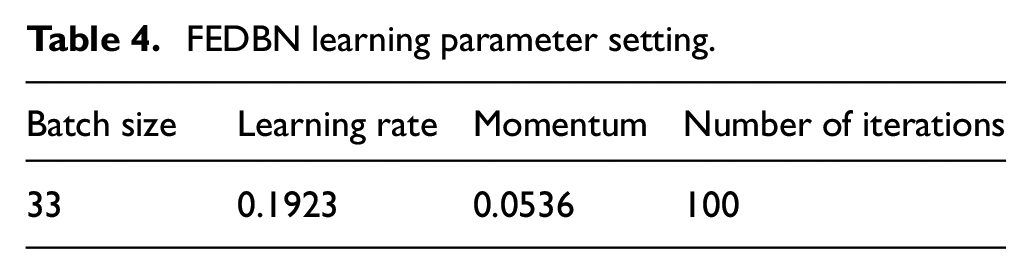
In addition, the three network structures tended to be stable at the 97th iteration. Although the RMSE of the three networks had a downward trend as the number of iterations increased, the calculation costs also increased significantly. Considering the effects of fault classification and calculation cost, the number of iterations was set to 100. Table 3 shows the setting of the FEDBN network structure parameters. The learning parameters obtained after optimization according to the SSA are listed in Table 4.
FEDBN structure parameter setting.
FEDBN learning parameter setting.
Different optimization algorithms used to optimize the results of the FEDBN network.
To characterize the feature classification ability of the optimized SSA-FEDBN model more intuitively, the output features of the improved FEDBN hidden and visible layers can be visualized using the t-SNE 39 clustering algorithm. As shown in Figure 8, four colors are used to indicate the four fault categories. The results show that, as the number of hidden layers increases, the effect of feature clustering improves significantly.
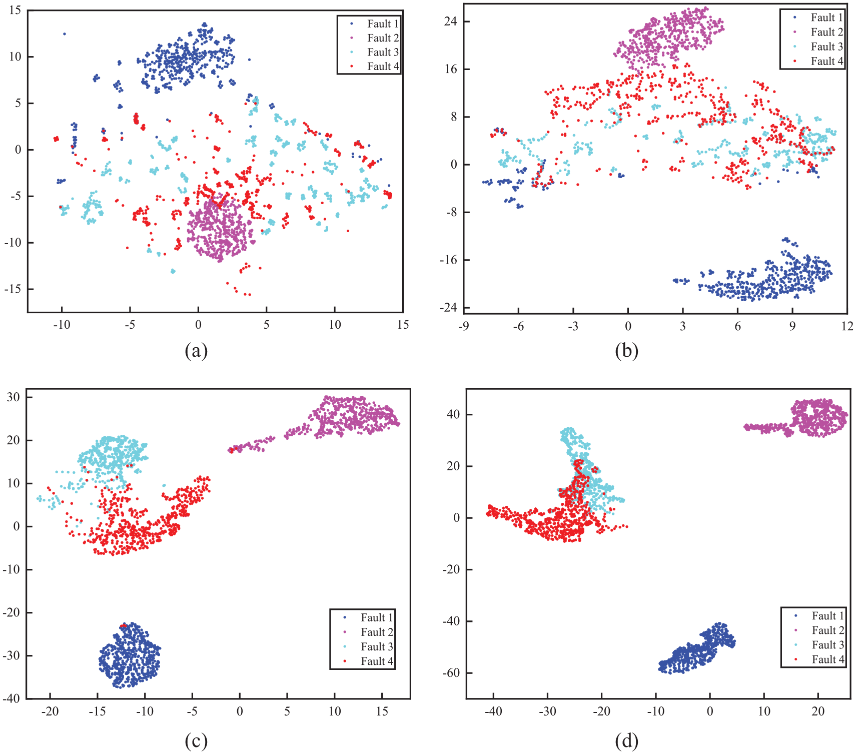
Visualizing the features of each hidden and visible layer through t-SNE: (a) first-level features, (b) second-level features, (c) third layer of features, and (d) visible-layer features.
To represent the classification effect of the four types of fault for RSGCs based on the SSA-FEDBN network, Figure 9 shows the classification confusion matrix for the test set. The horizontal axis of the confusion matrix represents the predicted failure category of the RSGC, and the vertical axis of the confusion matrix represents the actual failure category of the RSGC. The value on the diagonal line represents the correct rate of each classification of the SSA-FEDBN network in the test dataset. The off-diagonal line represents the error rate of the category. The experimental results show that the SSA-FEDBN diagnostic method has high diagnostic accuracy for four typical faults of RSGCs: 92.69%, 93.70%, 91.58%, and 93.15%, respectively.
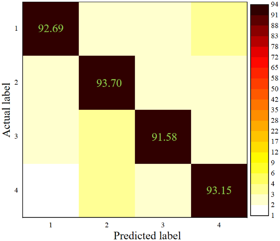
Confusion matrix diagram of classification results of four types of failure sample.
Comparison of diagnosis results
Comparison with other optimization methods
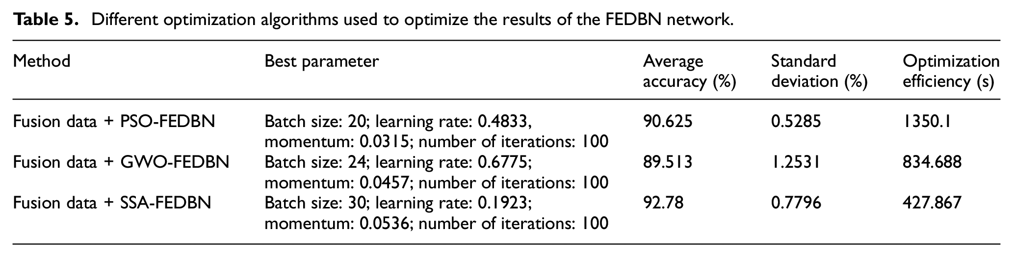
Particle swarm optimization (PSO) and gray wolf optimization (GWO) were used to optimize the structural parameters of the FEDBN network. The GWO-FEDBN parameter settings are as follows. The wolf number was set to 10, the maximum iteration number was 100, and the penalty parameter and kernel parameter were [0.01,1] and [0,1000], respectively. The PSO-FEDBN parameter setting was as follows. The population size was 20, the number of iterations was 50, the learning factor was 2, and the inertia weight was 0.8. The batch size and learning rate in the FEDBN model were obtained after optimization using GWO and PSO. As shown in Table 5, the recognition rate of SSA-FEDBN in all states reached more than 91%. For the three parameters, the optimized FEDBN and SSA-FEDBN had the best average detection rate (92.78%) and standard deviation (0.7796%). The experiment was repeated 20 times for the corresponding procedures for each method. The diagnosis result diagram is shown in Figure 10. To demonstrate the accuracy and adaptability of the SSA to tune the FEDBN network, Figure 10 shows that this method performed better than the other methods.
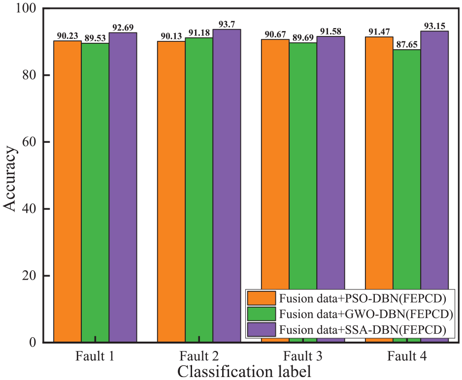
Comparison of FEDBN optimization results with different optimization algorithms.
The experimental results show that, compared with that of the other two FEDBN models, the comprehensive performance of the proposed method has advantages in terms of detection accuracy, stability, and computational efficiency.
Comparison with deep-learning methods
Two deep learning-methods, unoptimized FEDBN and CNN, were selected for comparison with the SSA-FEDBN method. The specific parameter settings are as follows.
FEDBN: A gradual decrease was adopted in the neuron selection strategy. To ensure that the network structure was 65-100-60-50-30-4, the number of iterations was set to 40, and the learning rate was set to 0.1.
CNN: The established CNN network consisted of one input layer, three convolution layers, three pooling layers, one fully connected layer, and one output layer. The cores of the convolutional layer were selected to be 7 × 7, 5 × 5, and 3 × 3, and the step size was 1. The sampling layer used the 2 × 2 kernel corresponding to the number of convolution layers, and the step size was 2. The fully connected layer was set to 512 nodes.
The original signal and the data processed by data fusion technology were input into the FEDBN, CNN, and SSA-FEDBN networks. The experiment was repeated 20 times for the corresponding procedures for each method, and the diagnosis result diagram is shown in Figure 11. The figure shows that, compared with the original FEDBN and CNN methods, the proposed one can diagnose faults with higher accuracy. In addition, the figure shows that, based on the fused data, the average test accuracy of the SSA-FEDBN method was 92.78%. The classification effect of the SSA-FEDBN RSGC fault diagnosis method based on raw data was also higher than that of the other diagnosis methods based on raw data. The original data were input into the CNN, FEDBN, and SSA-FEDBN algorithms, and the average training accuracy and training accuracies were not more than 75%. Therefore, the method proposed in this study can better reflect the fault situation and has the best classification performance.
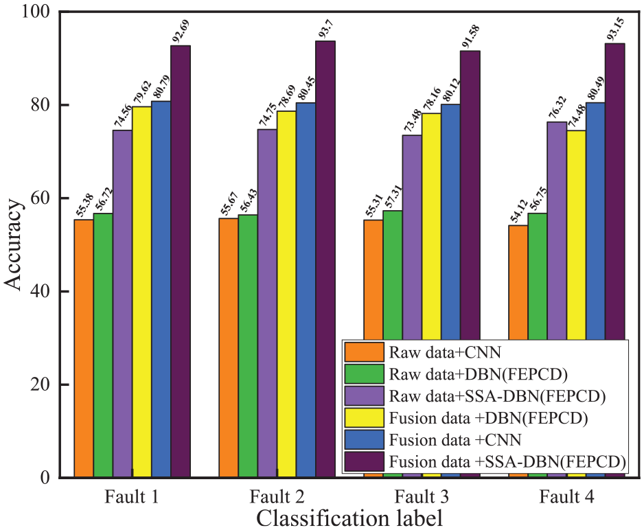
Comparison of deep-learning methods.
Comparison with traditional methods
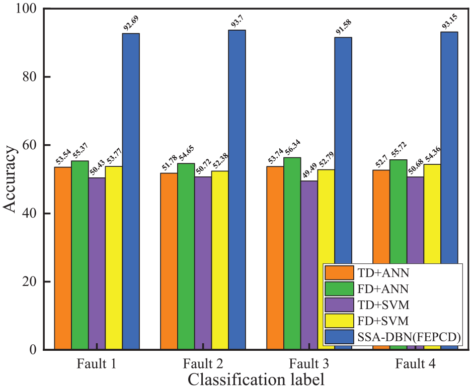
Traditional fault diagnosis methods for reciprocating machinery often include a feature extraction process based on manual operations, requiring personnel with certain prior knowledge to perform preprocessing operations on the sensor signals of the operating equipment. Feature information is extracted and selected to reflect the operating state of the equipment from the original sensor signal and perform fault identification based on the selected effective features. In this study, the time domain signal and frequency domain40,41 signal were chosen as the input signal of the traditional fault diagnosis method for comparison with the proposed method. The experiment was repeated 20 times for the corresponding procedures for each method. The diagnosis result diagram is shown in Figure 12. The parameters of the ANN and SVM were set as follows.
Comparison of traditional methods.
ANN: The ANN has a single hidden layer, and the number of hidden-layer neurons is 100.
SVM: The kernel function used was the radial basis function. According to the grid optimization results, the penalty coefficient was set to 16, the gamma function radius was g = 0.015625, and the stop training error accuracy was set to 1 × 10. 3
Figure 12 shows the diagnostic results of the proposed and conventional methods. This can be explained in two ways.
First, because of a lack of experience, hand-designed features may be restricted or even unusable. However, the diagnosis method based on deep learning can adaptively extract features without professional knowledge, making it possible to extract salient features for different faults. Second, most traditional fault diagnosis methods belong to the shallow fault diagnosis model, which cannot effectively reflect the fault characteristics of reciprocating shale gas compression; therefore, this reduces the diagnostic performance.
Conclusion
To address such problems as the complex structure and operating environment of the RSGC and the difficulty of extracting characteristic parameters, a RSGC fault diagnosis method based on the SSA adaptive optimization of the FEDBN network structure parameters was developed. The research results show the following. (1) The SSA algorithm adaptively adjusted to the structural parameters of the FEDBN network, which avoids the problems of a long manual adjustment time and poor diagnostic performance. (2) The fault diagnosis method of a RSGC based on the SSA-FEDBN can adaptively extract the fault features in the fusion signal. It solves the problem of relying excessively on signal-processing methods and prior knowledge in traditional fault diagnosis. The fault diagnosis ability is improved to a certain extent, and the proposed method has a stronger generalization performance and more advantages. (3) The proposed method was verified by collecting four types of failure data from a factory. The results show that the fault classification accuracy rate of the fault diagnosis model of a RSGC based on the SSA-FEDBN is as high as 92.78%. (4) Compared with the traditional DBN network, the ANN, SVM, CNN, and other algorithms, the SSA-FEDBN network has a stronger learning ability and obvious classification advantages when dealing with nonlinear weak fault signals. The accuracy is increased by approximately 10%–40%, which solves the problem of the low accuracy of traditional algorithms and shallow neural networks in RSGC fault diagnosis. This proves the superiority of this method in unsupervised feature learning and multisource information fusion.
Footnotes
Declaration of conflicting interests
The author(s) declared no potential conflicts of interest with respect to the research, authorship, and/or publication of this article.
Funding
The author(s) disclosed receipt of the following financial support for the research, authorship, and/or publication of this article: We acknowledge financial support from the National Key Research and Development Program of China (2021YFC2800903), International Science and Technology Cooperation Project Funding of Chengdu (2020-GH02-00041-HZ), Sichuan Science and Technology Program (2022ZHCG0052; 2022ZHCG0048), National Natural Science Foundation of China (52004235), China Postdoctoral Science Foundation (2020M683359), and China Postdoctoral Innovative Talents Support Program (BX20190292).
Data availability statement
The data that support the findings of this study are available from the corresponding author upon reasonable request.