Sage Journals: Discover world-class research

Abstract

For effectively predicting the tank failure time and analyzing the key elements influencing the reliability of corroded bottom plates, this article presents a model for calculating the reliability of corroded tank bottom plates based on a hierarchical Bayesian corrosion growth model. Firstly, the growth of corrosion defect depth is expressed by the gamma process, and the hierarchical Bayesian model is used to calculate the corrosion depth growth. After that, the reliability calculation model of the corroded tank base plate is established by combining the results of the hierarchical Bayesian model with the stress-strength interference theory, and the three uncertain factors of the base plate thickness, radius, and yield strength are considered in the model. Finally, the reliability assessment and sensitivity analysis of corroded bottom plate are carried out. The results show that the proposed reliability calculation model can provide more accurate failure state prediction results than the reliability calculation model which only considers the influence of corrosion depth, and can provide reference for reducing the failure rate of tank floor and reasonably formulating the maintenance plan of tank floor.

Keywords

Tank bottom plate corrosion defect depth hierarchical Bayesian model reliability analysis

Introduction

As a high quality and important energy source, oil is the main source of energy consumption at present, accounting for about 45%–46% of primary energy consumption.¹ In the past few years, with the continuous growth of crude oil demand and the volatility of the global crude oil market, the safety reserve of crude oil has become a global concern.^2,3 As an important facility in the petrochemical industry, storage tanks can store a large number of flammable and explosive substances, and play a pivotal role in the chemical production and oil storage and transportation system.^4,5 The storage tank in service by the environment and the impact of changes in operating conditions, some of the damage caused by corrosion will gradually accumulate, which may ultimately result in serious safety incidents.⁶ In particular, the corrosion status of the tank floor is a decisive factor affecting the safe running of the tank, the corrosion perforation of the tank floor will lead to tank failure, is the major element endangering the proper operation of the tank.⁷ At present, enterprises pursue the refinement and efficiency of the management of storage tanks, so the development of tank bottom corrosion state prediction technology is particularly important.

Corrosion depth value as an important factor in the assessment of corrosion status, there have been many scholars for the corrosion depth prediction of the bottom of storage tanks. Chen⁸ used probability statistics to study the relationship between corrosion and time on the bottom of the storage tank, the study shows that the maximum depth distribution of corrosion pits obey the law of extreme value distribution. Xiao et al.^9,10 established a reliability prediction model and a reliable life calculation model under the condition that the corrosion depth distribution obeys the extreme value type I maximum distribution. Liu et al.¹¹ carried out extreme value statistics on the maximum depth of corrosion at the bottom of the tank, and the results showed that: the extreme value III type distribution can better fit the statistical law of the maximum depth of corrosion at the bottom of the tank than the extreme value I type distribution. Zhu et al.¹² used a modified model of the gray dynamic model GM(1,1) to perform gray dynamic simulation of the actual statistical corrosion rate data of storage tanks. Liu and Zhang¹³ proposed an improved first-order univariate gray prediction model (IGM(1,1) model) for tank bottom corrosion prediction. However, in practical engineering, due to the limitations of the inspection tools, a sufficient number of samples may not be collected, and the prediction results will be problematic when the overall number of defect samples is so low that the extreme value distribution cannot be fitted precisely.¹⁴ The grey theory prediction model is only suitable for short-term prediction and has poor accuracy for medium and long-term prediction. In contrast, prediction of corrosion depth variation by Bayesian methods effectively avoids bias due to insufficient data, and its application in pipeline remaining life prediction and risk analysis has been effective. For example, Maes et al.¹⁵ proposed a hierarchical Bayesian framework for corrosion defect expansion considering the uncertainties in the pipeline deterioration process, and combined hierarchical Bayesian analysis with likelihood estimation methods for remaining life estimation. Zhou et al.^16–20 used power law process, gamma process, nonparametric Bayesian network model, and dynamic Bayesian network model to simulate the corrosion defect growth, respectively, and the results showed that these models can accurately and effectively predict the corrosion depth growth of defects. Aulia et al.^21,22 developed a dynamic Bayesian network model to forecast the future corrosion state for the corrosion of submarine pipelines, which provides an effective alternative for the residual lifetime prediction of corroded pipelines. In previous studies, Bayesian methods have not been widely applied in the field of storage tanks. Therefore, this paper draws on the application of Bayesian methods in pipeline corrosion prediction and applies Bayesian methods to tank bottom corrosion prediction.

The study of structural reliability theory has been developed more maturely so far, and the trend of the probability of failure during the degradation of the equipment can be predicted intuitively through the calculation of the variation of the reliability of the equipment, thus reducing the number of inspections to save the expenditure of manpower and material resources. Although reliability assessment has been widely used in other fields, the application for corroded tank bottoms is still relatively small. The reliability assessment of corroded tank bottoms in the current literature^8–11 is based only on the relationship between depth of corrosion and allowable residual thickness. However, in reality, the thickness, radius, and yield strength of the tank floor will deviate within a certain range during the design and manufacturing process, and these uncertainties will also affect the variation of reliability, which should be taken into account in the reliability assessment. Therefore, the stress-strength interference theory should be used to develop a model to fully consider the effects of uncertainties in the actual operating conditions.

In this paper, a reliability assessment method for tank bottom plates based on a hierarchical Bayesian corrosion growth model is proposed. The method uses Bayesian method instead of the traditional extreme value theory method for corrosion depth prediction, avoiding the problems arising from insufficient inspection data, while taking into account the errors arising from three uncertainties in the production design of the tank bottom plate thickness, radius, and yield strength, the reliability calculation model of the corroded tank bottom plate is established according to the stress-strength interference theory, and finally the three uncertainties are addressed sensitivity analysis. The calculation results of the model can provide a reference for the maintenance plan of corroded tank bottom to reduce the company’s expenditure on tank maintenance and inspection.

Model building

Hierarchical Bayesian corrosion growth model

Since the detection of etch depth in practical engineering is often limited by the detection tools, the sample capacity is difficult to reach large samples, and the sample data lack representativeness, the accuracy of the results is not guaranteed if the traditional extreme value theory is used for prediction.²³ Therefore, it is more reasonable to use a Bayesian approach applicable to small samples. The gamma process, which is applicable to expressing the monotonic increase of performance degradation over time, is also combined into the Bayesian method as a way to build a hierarchical Bayesian corrosion growth model to provide more accurate prediction results.

Gamma process

The gamma process has the properties of non-negative, smooth growth, and independent incremental processes, which are widely used for the description of degradation processes such as wear and corrosion, and it has good mathematical properties for easy convolution processing.²⁴ So the gamma process is well suited for describing the monotonically growing process of corrosion defect growth at the bottom of the tank with a probability density function of :

f_{G} (d | α, β) = \frac{β^{α} d^{α - 1} e^{- β d} I_{G}}{Γ (α)}

(1)

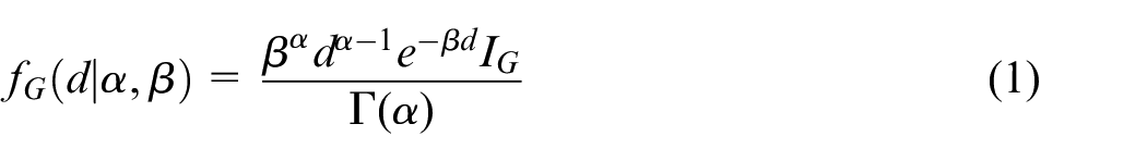
α and β represent the shape parameter and the inverse scale parameter of the gamma distribution, and I_G denotes an indicator function, I_G = 1 when d > 0 and I_G = 0 otherwise, and Г(α) denotes the gamma function.²⁵

Corrosion growth model

From the gamma distribution equation, the corrosion growth for two consecutive corrosion inspections follows a gamma distribution with a probability density function of:

f_{G} (Δ d_{j} | Δ α_{j}, β) = \frac{β^{Δ α_{j}} Δ d_{j}^{Δ a_{j} - 1} e^{- β Δ d_{j}}}{Γ (Δ α_{j})}

(2)

where j denotes the number of corrosion inspections, Δd_j is the corrosion increment of two adjacent inspections, β is the inverse scale parameter associated with the corrosion defect characteristics, Δα_j is the shape parameter associated with Δd_j, and the expression for Δα_j is:

Δ α_{j} = α (t_{j} - t_{0}) (j = 1)

(3)

Δ α_{j} = α (t_{j} - t_{j - 1}) (j = 2, 3, \dots, n)

(4)

where t₀ denotes the time when corrosion defects start to be generated and t_j denotes the time of the jth corrosion inspection.

The predicted corrosion depth for each inspection is the sum of the corrosion depth at the previous testing and the corrosion increment at the jth testing, and assuming that the corrosion defect depth at time₀t is 0, the expression for the predicted corrosion depth at the jth inspection is:

d_{j} = d_{j - 1} + Δ d_{j}

(5)

All variables of the above corrosion growth model can be represented by a three-level Bayesian model, and the hierarchy of the model is shown by a directed acyclic graph.²⁶ As shown in Figure 1, the rectangular boxes represent the known parameters, which include the prior information of α, t₀, β, that is, the hyperparameters a₁, b₁, a₂, b₂, a₃, b₃ and the time to perform corrosion detection. The oval boxes represent the random variables, that is, α, t₀, β three parameters to be estimated. The first layer parameters are the basic parameters of the model, the second layer parameters are the corrosion growth for two consecutive corrosion inspections and the shape parameters of the model, and the third layer parameters are the predicted corrosion depth at the jth inspection.

Figure 1.

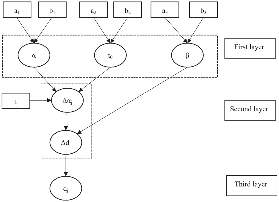
Hierarchical Bayesian model.

Parameter prior distribution

The prior distribution of α and β is set to the gamma distribution, because the gamma distribution ensures that α and β are positive amounts and can be used as an uninformative prior distribution.²⁷ The prior distribution of t₀ is set to a uniform distribution. The lower bound is zero and the upper bound is the time interval from the start of the tank being put into service to the first inspection. And the prior distributions of β and t₀ are assumed independent of each other.

Parameter posterior distribution

The expressions for the conditional posterior distributions of α, t₀, and β are as follows²⁸:

\ln [p (α | Δ d, β, t_{0}, a_{1}, b_{1})] \propto \sum_{j = 1}^{n} [Δ α_{j} \ln (β) + (Δ α_{j} - 1) \ln (Δ d_{j}) - \ln (Г (Δ α_{j}))] + (a_{1} - 1) l n α - α b_{1}

(6)

\begin{matrix} \ln [p (t_{0} | Δ d, α, β, a_{2}, b_{2}) \propto α (t_{1} - t_{0}) \ln β \\ + [α (t_{1} - t_{0}) - 1] \ln (Δ d_{1}) - \ln (Γ (α (t_{1} - t_{0}))) \end{matrix}

(7)

p (β_{i} | Δ d, α, t_{0}, a_{3}, b_{3}) \propto f_{G} (α (t_{n} - t_{0}) + a_{3}, \sum_{j = 1}^{n} Δ d_{j} + b_{3})

(8)

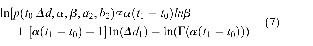
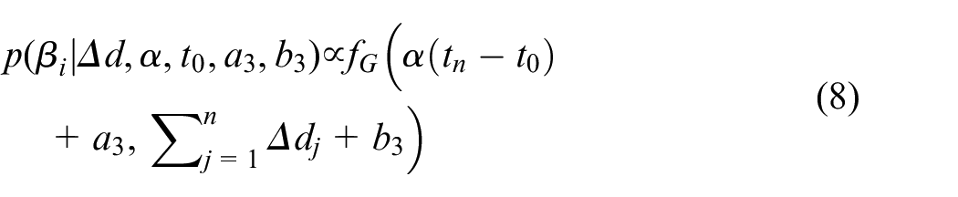
Since the conditional posterior distributions of α and t₀ cannot be obtained directly from the functional equations, this paper uses a grid estimation method to evaluate the conditional posterior distributions of α and t₀ by sampling the functional equations.

Stress concentration factor modeling

Stress concentration refers to the geometric discontinuity of the force member causes the stress distribution in the adjacent area to change, causing a significant increase in the local range of stress phenomenon. When the bottom plate of a tank containing corrosion defects is subjected to external load, stress concentration will occur at the edges of the defects, causing the strength of the bottom plate to decrease and the safety performance to be reduced. Therefore, it is very important to study the connection between the factor of stress concentration and the corrosion depth. The expression of the factor of stress concentration is:

K = \frac{σ_{\max}}{σ_{m}}

(9)

of which:

$σ_{\max}$ is the maximum stress value, Pa.

$σ_{m}$ is the membrane stress value, Pa.

In this paper the stress concentration phenomenon is analyzed using finite element analysis. ANSYS software is used to build a model based on the actual dimensions of the tank, and the geometric model is meshed using Solid185 cells, fixed constraints are applied to the tank bottom, and hydrostatic pressure is applied to the tank wall and the interior of the tank bottom. The corrosion depth was set to increase gradually from 1 mm to solve the stress distribution at the corrosion defect. After obtaining the stresses at the defect, the stress linearization tool was used to decompose the stresses along the path through the hazardous section to obtain the film stress values and maximum stress values along the path.

Reliability calculation model

Stress-strength interference model

In mechanical reliability design, the stress-strength interference theory is often used to calculate the reliability of a part, which can be obtained by specific numerical calculations of the reliability of the component.²⁹ The probabilistic design method based on stress-strength interference theory treats stress and strength as random variables, which is realistic.³⁰ The probability of failure increases from zero when the stress to which the part is subjected is greater than the strength of the material. The full likelihood that the stress is greater than the strength is the probability of failure, and is expressed as:

P (S > R) = P [(Z = R - S) < 0]

(10)

Conversely, the reliability is obtained and the expression is given as:

P (S < R) = P [(Z = R - S) > 0]

(11)

where Z denotes the limit state equation, R denotes the strength index, and S denotes the load index.

Limiting state equation

In this paper, the probability of failure is used to characterize the corrosion state condition of the bottom plate, and the stress concentration factor, yield strength, and residual thickness are used to characterize the strength variation of the tank bottom plate. Since the load on the bottom plate is mainly from the liquid inside the tank and the tank wall, the hydrostatic pressure and the self-weight of the tank are used to characterize the load applied to the bottom plate. The expression of the limit state equation is given by:

Z = K * σ * \frac{h - d}{h} - [ρ_{l} gL + \frac{ρ gH (R^{2} - r^{2})}{R^{2}}]

(12)

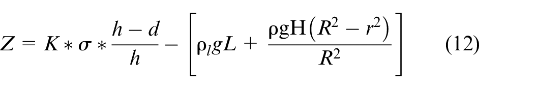
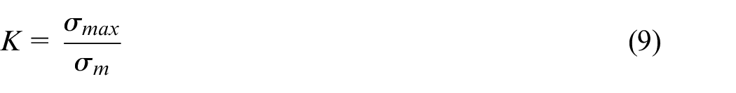
where:

K is an expression for the stress concentration factor, given in Section “Calculated results of hierarchical Bayesian corrosion growth model”;

σ is the yield strength of the base plate, MPa;

h is the thickness of the substrate, m;

d is the depth of corrosion, m;

$ρ_{l}$ is the density of the liquid, kg/m ³;

$ρ$ is the density of the steel, kg/m ³;

H is the height of the tank, m;

R is the radius of the base plate, m;

r is the internal diameter of the tank, m.

Model validation

Hierarchical Bayesian model accuracy validation

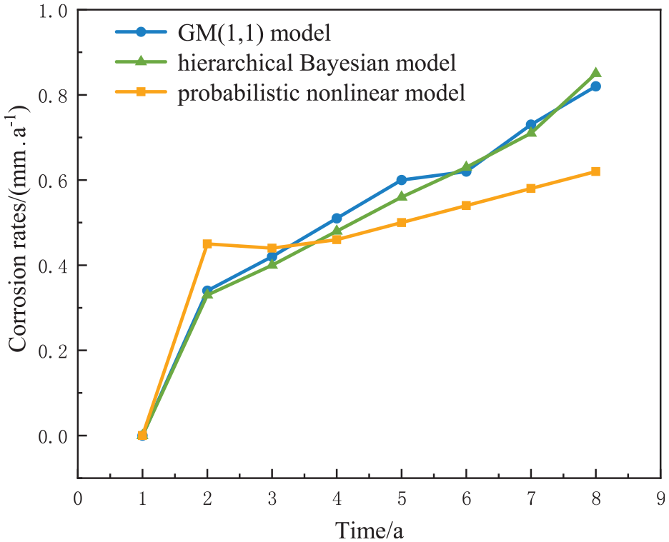
In the present study, the GM(1,1) model is usually considered to be a more accurate corrosion prediction method.^31–35 Therefore, the corrosion detection data in the literature¹² were selected and the results of the GM(1,1) model in the literature were used as the standard to verify the precision of the hierarchical Bayesian model by contrasting the results of the hierarchical Bayesian model and the probabilistic nonlinear model proposed in the literature³⁶ with the results of the GM(1,1) model. The results are shown in Figure 2.

Figure 2.

Comparison of the results of the three models.

From the figure, it can be observed that the predictions of corrosion rates from the hierarchical Bayesian and GM(1,1) models are very close, while the predictions from the probabilistic nonlinear model vary considerably. Therefore, it can be concluded that the hierarchical Bayesian model has a fairly accurate predictive power.

Reliability verification of reliability calculation models

The tank corrosion test data from the literature³⁷ were selected and the model developed in this paper was compared with the calculation method used in the literature.¹¹ The method used in the literature, which considers only the relationship between corrosion depth and allowable remaining thickness, is given by the following equation:

Z = h - d - h_{0}

(13)

where:

h is the thickness of the substrate, m.

d is the depth of corrosion, m.

h ₀ is the allowable residual thickness and is taken as h₀= 2.5m.

The results of the calculation are shown in Figure 3. The calculation computations of the stress intensity interference model show that the probability of failure of the tank in the 16th year of service is 0.0013, reaching the upper limit of the probability of failure, at which time the corrosion depth is 5.66 mm. The calculation results of the depth model show that the probability of failure of the tank in the 12th year of service is 0.001, reaching the upper limit of the probability of failure, at which time the corrosion depth is 4.25 mm. According to API653-2001, the minimum remaining thickness is 2.5 mm, and the depth model calculation results show that the remaining thickness of the tank at the time of failure is 3.75 mm, which is in accordance with the provisions of the standard.

Figure 3.

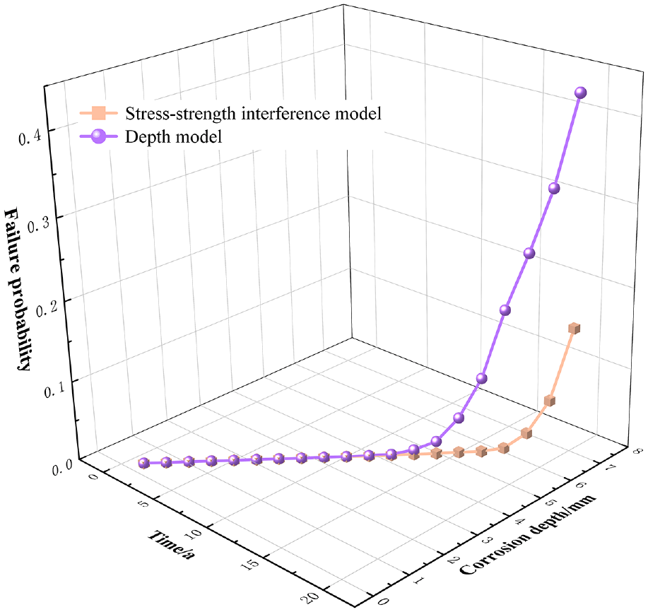
Comparison of the results of the two models.

Example applications

Introduction

The target of this paper is a crude oil storage tank in an oil transfer station, which has been in operation for 21 years from the time it was put into production use to the time of corrosion testing, the tank is a floating roof tank with a volume of 20,000 m³, 40.5 m in diameter, and 15.8 m in height. The tank bottom thickness is 6 mm and the yield strength is 490 MPa. Around 166 plates were tested for residual thickness, and the bottom of the tank was divided into 26 areas, and the results of the thickness measurement showed the average corrosion depth as shown in Figure 4.

Figure 4.

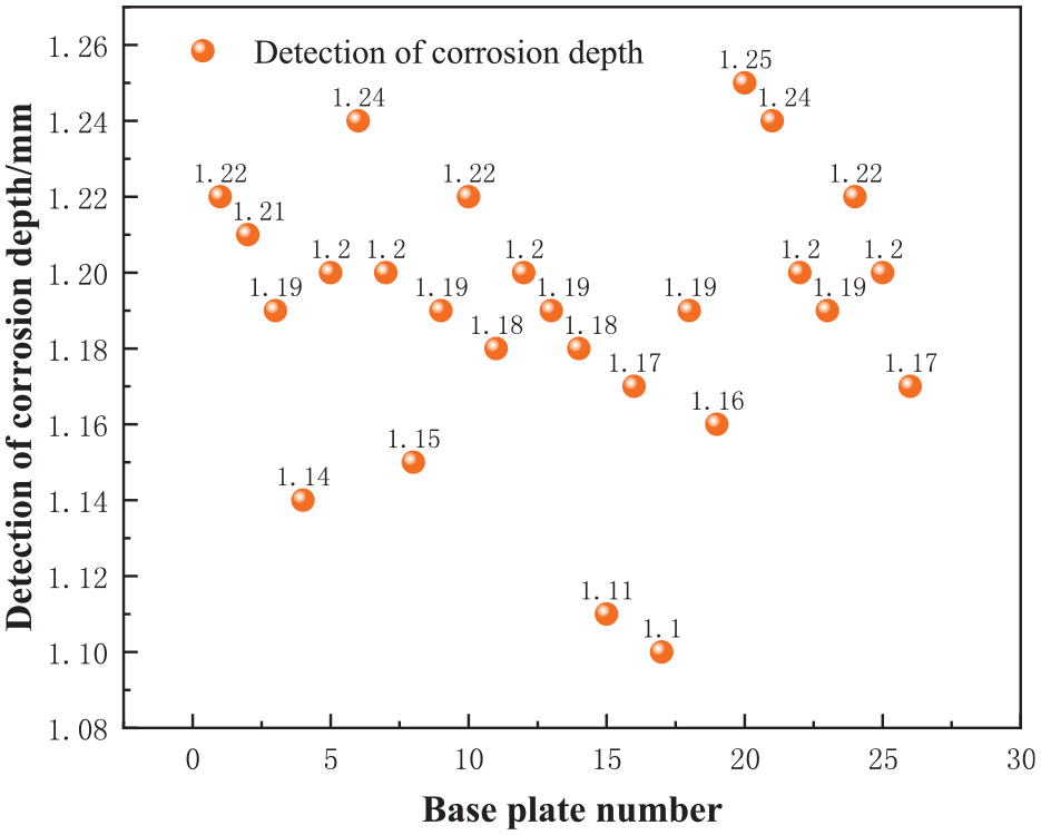
Thickness measurement data.

Calculated results of hierarchical Bayesian corrosion growth model

Based on the characteristics of the corrosion detection data in the inspection report, the prior distribution parameters of the hyperparameters were set as: a₁ = 1, b₁ = 1, a₂ = 0, b₂ = 3, a₃ = 1, b₃ = 0.06. A total of 10,000 Markov chain analog sequences were produced in the R language for gamma model parameter estimation. The first 5000 of these sequences are considered as the aging period and are discarded since the results of the Markov chain simulations of the aging period do not reach the smooth phase.³⁸ The samples from the remaining series were employed to assess the probability features of the parameters in the growth model.

The random parameters α, t₀, and β are assumed to be deterministic after parameter estimation and their values are the averages of the corresponding conditional posterior distributions after simulation. The predicted depth of corrosion depth is the mean depth evaluated from the gamma process. The predicted results are shown in Figure 5, where the predicted depth of the tank floor at the 21st year of service is 1.23 mm. The two dotted lines in the figure show the predicted corrosion depth ±10%. These two dotted lines are commonly used in the pipeline industry as confidence limits to check the accuracy of the tool, and are used in this paper as a measure for the prediction reliability of the corrosion growth model. Figure 5 shows that the prediction results based on the gamma process are extremely accurate, and the actual values of 24 out of 26 areas fall within the prediction range with a maximum absolute error of about 11%, so it can be assumed that the model can be used for corrosion depth prediction of the tank floor and has good accuracy.

Figure 5.

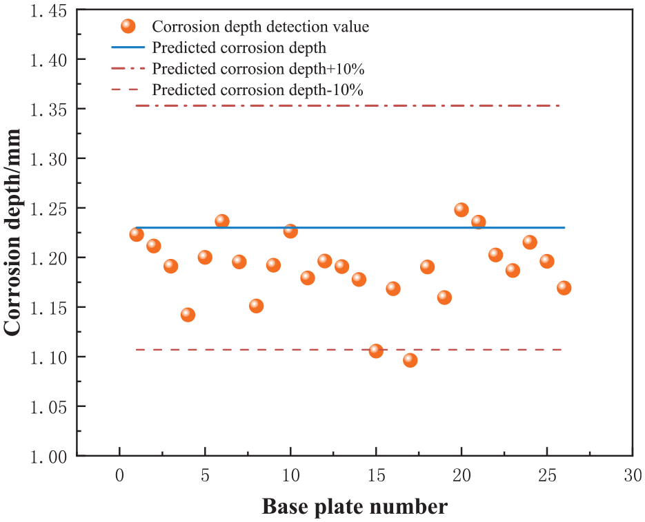
Predicted corrosion depth results.

Fitting of expressions for stress concentration factors

The finite element analysis was performed based on the tank data from the inspection report and the results are shown in Figure 6.

Figure 6.

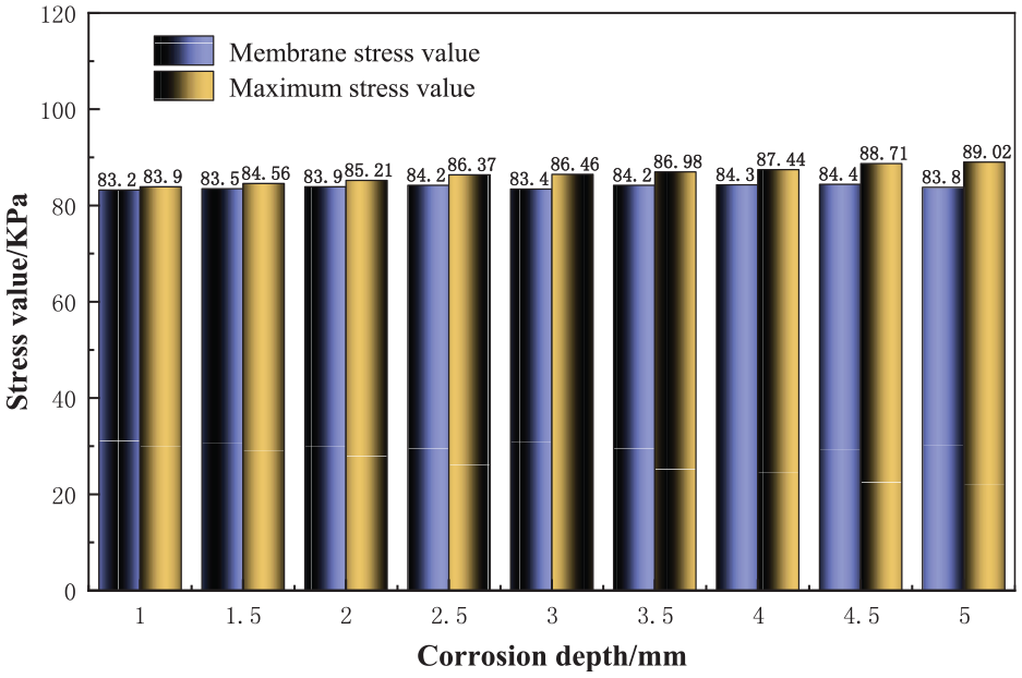
Stress linearization results.

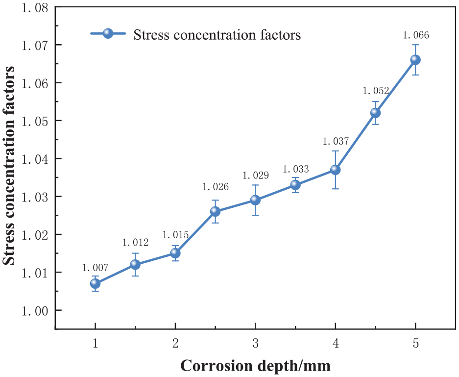
Taking the corrosion depth as the horizontal axis value and the factor of stress concentration as the vertical axis value, the relationship curve between the factor of stress concentration and the corrosion depth was drawn. From Figure 7, it can be seen that the factor of stress concentration and corrosion depth basically show a linear relationship, and the factor of stress concentration increases with the increase of corrosion depth. Therefore, a linear regression analysis was performed in SPSS software, and the following relationship equation was derived.

K = 0.014 d + 0.99

(14)

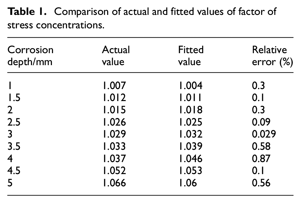
The depths of different defects are substituted into the fitted equation, and the fitted values of the factor of stress concentration are obtained as shown in Table 1, which shows that the fitted values are basically similar to the actual values. The maximum relative error is only 0.87%, which shows that the factor of stress concentration expression fitted in the paper can more accurately represent the stress concentration of corrosion defects.

Table 1.

Comparison of actual and fitted values of factor of stress concentrations.

Corrosion depth/mm	Actual value	Fitted value	Relative error (%)
1	1.007	1.004	0.3
1.5	1.012	1.011	0.1
2	1.015	1.018	0.3
2.5	1.026	1.025	0.09
3	1.029	1.032	0.029
3.5	1.033	1.039	0.58
4	1.037	1.046	0.87
4.5	1.052	1.053	0.1
5	1.066	1.06	0.56

Figure 7.

Factor of stress concentration versus corrosion depth.

Results of the probability of failure calculation

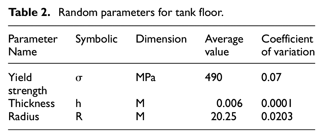
For the calculation of the failure probability this paper uses the Monte Carlo method,³⁹ the bottom plate yield strength, bottom plate thickness, and bottom plate radius in the limit state equation as random variables, and the corrosion depth is the Bayesian model from the previous section combined into the reliability calculation model, and assumes that all three random variables obey a normal distribution and are independent of each other, and the specific settings of the random parameters are shown in Table 2.

Table 2.

Random parameters for tank floor.

Parameter Name	Symbolic	Dimension	Average value	Coefficient of variation
Yield strength	σ	MPa	490	0.07
Thickness	h	M	0.006	0.0001
Radius	R	M	20.25	0.0203

The entire solution process is computed with the help of MATLAB tools. Using the powerful numerical computation capabilities of MATLAB, the probability of failure of the tank floor is calculated using direct Monte Carlo sampling in the MATLAB statistical toolbox.⁴⁰

MATLAB proceeds as follows.

(1) Set the number of times the tank floor should be inspected. $j \in [1, 17]$ Again, set to once every 3 years;

(2) Using the normal random number generation instruction, generate N (N is the total number of cycles, N = 30,000) sets of random numbers, respectively.

(3) Using the arithmetic functions of MATLAB, the generated random numbers are brought into the limiting state equation to obtain the value of Z.

(4) The number of statistics Z < 0 is noted as n. The probability of failure is $P (Z < 0) = n / N$ .

(5) Return to (2) and calculate the failure probability case for the following year.

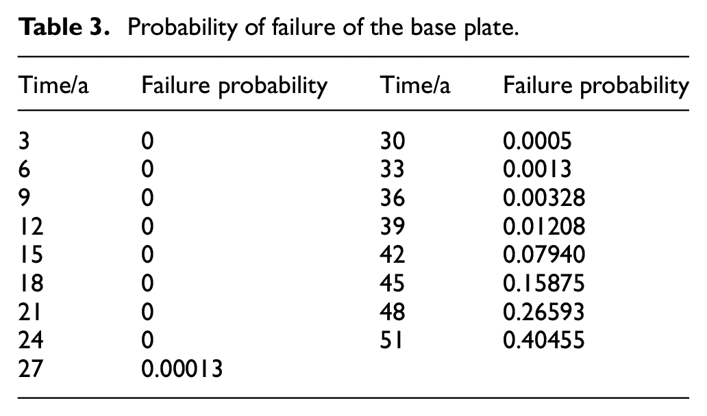
The results of the failure probability calculation and the probability of failure versus time are shown in Table 3 and Figure 8, from Table 3, it can be seen that the probability of failure of the tank base plate starts to occur in the 27th year of service and gradually increases, and the probability of failure reaches 0.0013 in the 33rd year, according to the standard API579, the upper limit of the probability of failure of in-service equipment is 10^–3 (i.e., the position of the line in Figure 8), so it can be It is determined that the bottom plate of this tank is in a failed state at the 33rd year of service, at which point it is the best time to make repairs and the bottom plate should be replaced or patched. The probability of failure can be seen to increase significantly after the 31st year, and the risk of failure of the tank bottom increases, and it is likely that an accident will occur due to untimely repair.

Table 3.

Probability of failure of the base plate.

Time/a	Failure probability	Time/a	Failure probability
3	0	30	0.0005
6	0	33	0.0013
9	0	36	0.00328
12	0	39	0.01208
15	0	42	0.07940
18	0	45	0.15875
21	0	48	0.26593
24	0	51	0.40455
27	0.00013

Figure 8.

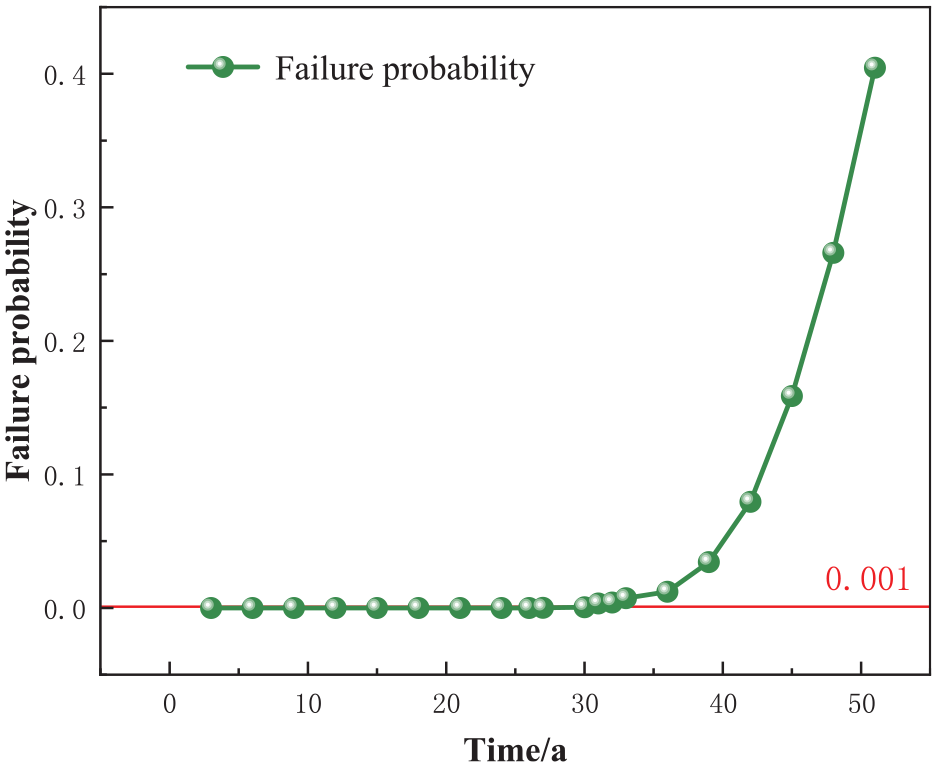
Plot of time versus probability of failure.

Again the model developed in this paper was compared with the results of the depth model and the results are shown in Figure 9. The depth model curve shows that the probability of failure of the tank in year 28 is 0.0011, which means the remaining life is 6 years. According to the inspection data, the tank was repaired in the 32nd year, which is basically consistent with the remaining life predicted in this paper, and it can be considered that the model built in this paper can get the prediction results closer to the actual working conditions than the depth model.

Figure 9.

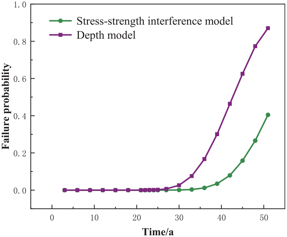
Comparison of failure probability of two models.

Sensitivity analysis

The purpose of the parametric sensitivity analysis of corroded substrates is to obtain several variables that have the greatest impact on the failure rate and to find the key factors for preventing substrate failure. By comparing the relative magnitude of the sensitivity indicators for each parameter, the key issues affecting the reliability of the structure are identified.⁴¹

The variation of failure probability under different parameter values is obtained by varying the values of three stochastic variables in the equation of limit state, and the same Monte Carlo method is used for the probability of failure calculation. The bottom plate thickness is designed with a corrosion margin, so the actual bottom plate thickness generally deviates from the design thickness by 1–2 mm, so the change values for the bottom plate thickness in this paper are 7 and 8 mm. 20,000 m³ tank bottom plate diameter specifications are generally around 40 m, so the change values for the bottom plate radius in this paper are 19.5 and 21 m. The yield strength change values are set in reference.⁴² The sensitivity analysis was carried out by varying the three random variables and keeping the other parameters constant, and the computational results are shown in Figures 10 to 12.

Figure 10.

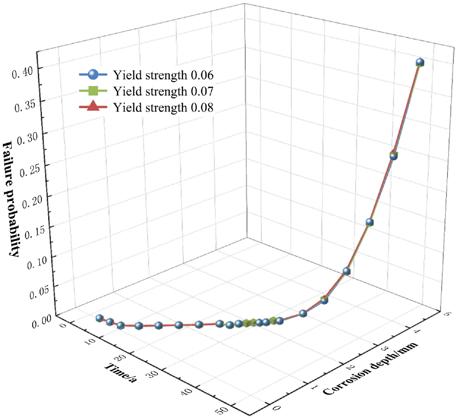
Sensitivity curves for coefficient of variation of yield strength.

Figure 11.

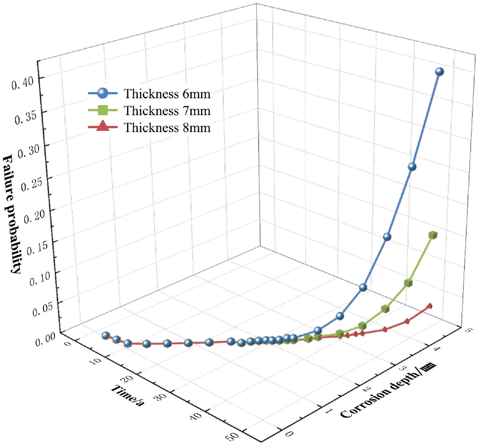
Sensitivity curves for base plate thickness.

Figure 12.

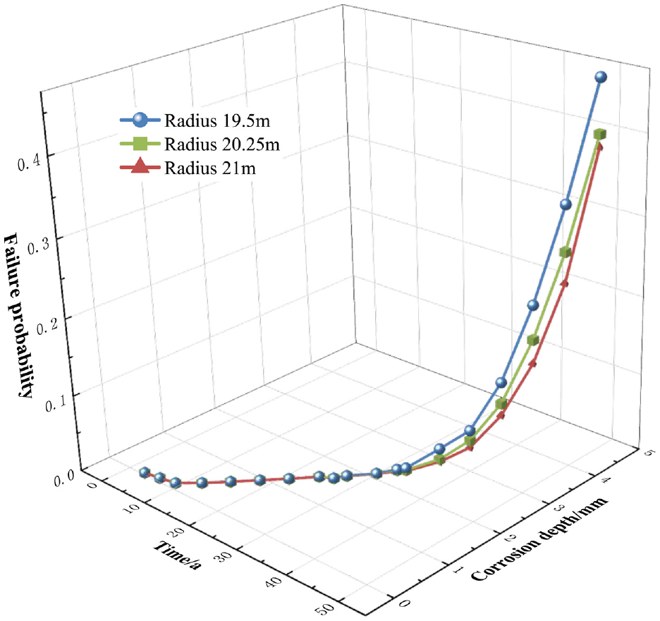
Sensitivity curves for base plate radius.

When only the yield strength coefficient of variation is varied, all three cases reach the upper limit of the probability of failure at year 31, and although the results show that the overall failure probability decreases slightly with greater yield strength, the three curves almost overlap as shown in Figure 10, which indicates that the change in the yield strength coefficient of variation has little effect on the probability of failure. When only the mean value of the bottom plate thickness is varied, the thicker the thickness the later the bottom plate fails, and as the service time increases, the effect of the thickness size on the failure probability becomes more and more significant, which shows that the mean value of the bottom plate thickness is the key factor affecting the failure probability. When only the mean value of the radius of the base plate is varied, the time of failure of the base plate becomes gradually larger when the radius of the base plate becomes larger, and the failure probability increases with time, the influence of the radius size on the probability of failure becomes more and more significant, but the degree of influence is not as obvious as the thickness of the base plate.

From the above analysis, the three uncertainty factors are obtained to affect the reliability in the order of base plate thickness > base plate radius > yield strength.

Conclusion

In this article, a reliability assessment approach for tank bottom plates based on layered Bayesian corrosion growth model is proposed. The growth of corrosion defects is simulated using a gamma process, and the corrosion depth growth is calculated by combining the hierarchical Bayesian approach and Markov chain Monte Carlo simulation. In the subsequent reliability analysis, the hierarchical Bayesian model is put into the reliability model together with the uncertainty factors of bottom plate thickness, radius, and yield strength, and the field inspection data of a tank is used as an example to compare with the results of the reliability calculation model that only considers the effect of corrosion depth. The calculation results show that the failure probability curve obtained from the reliability model in this paper reflects the residual lifetimes of the tank is 12 years, while the residual lifetimes predicted by the depth model is only 6 years, which is much different from the actual situation, so the model proposed in this paper can get the prediction results closer to the actual working conditions compared with the traditional depth model. The sensitivity analysis results show that the main factors affecting the variation of the reliability of the tank bottom plate in the reliability calculation model are the thickness and the radius, and the influence size is thickness > radius > yield strength, which shows that it is necessary to consider the uncertainty factors arising from the design and manufacture in the reliability analysis. The model proposed in this paper provides more accurate prediction results, which can provide reference for reducing the failure rate of tank bottom and developing a reasonable maintenance plan for the tank bottom.

Footnotes

Declaration of conflicting interests

The author(s) declared no potential conflicts of interest with respect to the research, authorship, and/or publication of this article.

Funding

The author(s) disclosed receipt of the following financial support for the research, authorship, and/or publication of this article: This work was supported by the Joint fund of Natural Science Foundation of Liaoning Province (Grant numbers 2020-HYLH-14) and Liaoning Provincial Scientific Research Program (Grant numbers LJKZ0395).

ORCID iD

Guilin Zhang

References

Wang

Tang

Yuan

, et al. An early warning system for oil security in China. Sustainability 2018; 10: 283.

Shao

Wang

, et al. Product environmental footprints assessment for product life cycle. J Cleaner Prod 2019; 233: 446–460.

Liu

Zeng

, et al. Product carbon footprint across sustainable supply chain. J Cleaner Prod 2019; 241: 118320.

Ding

Khan

Guo

, et al. A novel approach to reduce fire-induced domino effect risk by leveraging loading/unloading demands in chemical industrial parks. Process Saf Environ Prot 2021; 146: 610–619.

Guo

Jie

Khan

, et al. Fuzzy Bayesian network based on an improved similarity aggregation method for risk assessment of storage tank accident. Process Saf Environ Prot 2021; 149: 1031–1031.

Deif

Leier

Snow

, et al. Microwave sensor array for corrosion prediction in steel tank bottoms. In: 12th international pipeline conference (IPC 2018) Calgary, AB, Canada, 24–28 September 2018, vol. 1.

Feng

Yang

Huang

BQ.

Corrosion analysis and remaining useful life prediction for storage tank bottom. Int J Adv Rob Syst 2019; 16: 172988141987705.

Chen

SW.

A study on the probability statistics and assessment of tank bottom corrosion. Pet Reservoirs Fuel Stn 2012; 21: 2.

Xiao

Liu

YH.

Reliability calculation study of tank bottom plate corrosion. Corros Prot 2005; 26: 4.

10.

Xiao

LIu

, et al. Mathematical modeling of the reliability of corroded bottom plates of oil tanks. Oil Gas Storage Transp 2005; 24: 5.

11.

Liu

Zhang

Zhao

, et al. Application of extreme value theory to the corrosion depth statistics of oil storage tank bottoms. J Harbin Inst Technol 2013; 45: 5.

12.

Zhu

Chen

Prediction of corrosion rate of storage tanks based on improved model of grey system theory. Oil Gas Storage Transp 2010; 29: 4.

13.

Liu

Zhang

GY.

An improved grey model for corrosion prediction of tank bottom. Prot Metals 2007; 43: 407–412.

14.

Kuniewski

van der Weide

JAM

van Noortwijk

JM.

Sampling inspection for the evaluation of time-dependent reliability of deteriorating systems under imperfect defect detection. Reliab Eng Syst Saf 2009; 94: 1480–1490.

15.

Maes

Faber

Dann

, et al. Hierarchical modeling of pipeline defect growth subject to ILI uncertainty. In: 28th international conference on ocean, offshore and arctic engineering, Honolulu, HI, USA, 31 May 31–05 June 2009, vol. 2, pp. 375–384.

16.

Xiang

Zhou

WX.

Integrated pipeline corrosion growth modeling and reliability analysis using dynamic Bayesian network and parameter learning technique. Struct Infrastruct Eng 2020; 16: 1161–1176.

17.

Al-Amin

Zhou

WX.

Evaluating the system reliability of corroding pipelines based on inspection data. Struct Infrastruct Eng 2014; 10: 1161–1175.

18.

Al-Amin

Zhou

Zhang

, et al. Hierarchical Bayesian corrosion growth model based on in-line inspection data. J Pressure Vessel Technol Trans ASME 2014; 136.

19.

Xiang

Zhou

WX.

A nonparametric Bayesian network model for predicting corrosion depth on buried pipelines. Corrosion 2020; 76: 235–247.

20.

Qin

Zhou

Zhang

Bayesian inferences of generation and growth of corrosion defects on energy pipelines based on imperfect inspection data. Reliab Eng Syst Saf 2015; 144: 334–342.

21.

Aulia

Tan

Sriramula

Prediction of corroded pipeline performance based on dynamic reliability models. In: 26th CIRP conference on life cycle engineering (LCE), West Lafayette, IN, USA, 7–9 May 2019, pp. 518–523.

22.

Aulia

Tan

Sriramula

Dynamic reliability analysis for residual life assessment of corroded subsea pipelines. Ships Offshore Struct 2021; 16: 410–422.

23.

Pesinis

Tee

KF.

Bayesian analysis of small probability incidents for corroding energy pipelines. Eng Struct 2018; 165: 264–277.

24.

de Almeida

Ramos

Rao

, et al. Objective Bayesian inference for the capability index of the Gamma distribution. Qual Reliab Eng Int 2021; 37: 2235–2247.

25.

Lima

CHR

Kwon

Kim

YT.

A Bernoulli-Gamma hierarchical Bayesian model for daily rainfall forecasts. J Hydrol 2021; 599: 126317.

26.

Wang

Zhang

Qin

GJ.

Reliability evaluation of local corrosion of X80 pipeline subjected to accidental earthquake considering geotechnical discontinuities. Int J Pressure Vessels Pip 2021; 189: 104254.

27.

Castelletti

Bayesian model selection of gaussian directed acyclic graph structures. Int Stat Rev 2020; 88: 752–775.

28.

Zhang

Zhou

WX.

System reliability of corroding pipelines considering stochastic process-based models for defect growth and internal pressure. Int J Pressure Vessels Pip 2013; 111: 120–130.

29.

Jana

Kumar

Chatterjee

, et al. Estimating stress-strength reliability for exponential distributions with different location and scale parameters. Int J Adv Eng Sci Appl Math 2021; 13: 177–190.

30.

Bai

Balakrishnan

, et al. Statistical inference for dependent stress-strength reliability of multi-state system using generalized survival signature. J Comput Appl Math 2021; 390: 113316.

31.

Qin

Liu

Chen

Pipeline corrosion prediction based on an improved artificial bee colony algorithm and a grey model. J Beijing Univ Chem Technol 2021; 48: 74–80.

32.

Qiao

Zhu

, et al. Research on damage and deterioration of fiber concrete under acid rain environment based on GM(1,1)-Markov. Materials 2021; 14: 6326.

33.

Wang

Sun

QW.

Nonlinear total least-squares variance component estimation for GM(1,1) model. Geodesy Geodyn 2021; 12: 211–217.

34.

Zhao

Shi

Oil-gas cost in the declining period predicting model based on self-adaptive GM(1,1,lambda). In: 2021 6th international conference on intelligent computing and signal processing (ICSP), Xi an, China, 9–11 April 2021, pp. 69–72.

35.

Comert

Begashaw

Huynh

Improved grey system models for predicting traffic parameters. Expert Syst Appl 2021; 177: 114972.

36.

Sun

Wang

, et al. Bayesian-based corrosion depth prediction method for gas pipelines. Oil Gas Storage Transp 2019; 38: 8.

37.

Zhu

, et al. Corrosion inspection and integrity evaluation of large diesel storage tanks. Petrochem Corros Prot 2019; 36: 5.

38.

Zhang

Development of probabilistic corrosion growth models with applications in integrity management of pipelines. Ontario: The University of Western Ontario, 2014.

39.

Abyani

Bahaari

MR.

A comparative reliability study of corroded pipelines based on Monte Carlo Simulation and Latin Hypercube Sampling methods. Int J Pressure Vessels Pip; 181: 104079.

40.

Park

Lee

Kim

, et al. Comprehensive framework for underground pipeline management with reliability and cost factors using Monte Carlo simulation. J Loss Prev Process Ind 2020; 63: 104035.

41.

Mao

Lang

Chen

, et al. Improving source inversion performance of airborne pollutant emissions by modifying atmospheric dispersion scheme through sensitivity analysis combined with optimization model. Environ Pollut 2021; 284: 117186.

42.

Stress and reliability analysis of corrosion defects in Suizhong 36-1 terminal crude oil storage tank. Cheng Du: Southwest Petroleum University, 2015.

Reliability assessment method for tank bottom plates based on hierarchical Bayesian corrosion growth model

Abstract

Keywords

Introduction

Model building

Hierarchical Bayesian corrosion growth model

Gamma process

Corrosion growth model

Parameter prior distribution

Parameter posterior distribution

Stress concentration factor modeling

Reliability calculation model

Stress-strength interference model

Limiting state equation

Model validation

Hierarchical Bayesian model accuracy validation

Reliability verification of reliability calculation models

Example applications

Introduction

Calculated results of hierarchical Bayesian corrosion growth model

Fitting of expressions for stress concentration factors

Results of the probability of failure calculation

Sensitivity analysis

Conclusion

Footnotes

Declaration of conflicting interests

Funding

ORCID iD

References