Sage Journals: Discover world-class research

Abstract

Unstructured technical texts are a rich resource of engineering knowledge underutilised for data analysis. Maintenance work orders (MWO), for example, capture valuable information to inform what work was done on an asset and why. Data in MWO short text fields is unstructured, terse and jargon-rich, complicating the ability of both humans and machines to read it. Our challenge is to efficiently extract technical information from the MWO short text field and combine it with data in structured fields such as dates, functional location, make and model of the asset. In this paper we present a technical language processing-based solution for this problem. Echidna is an intuitive query-enabling interface that visualises historic asset data in the form of a knowledge graph. This knowledge graph is produced by MWO2KG, which uses deep learning supported by annotated training data to automatically construct knowledge graphs from unstructured technical text combined with data from structured fields. The tools are tested on maintenance work order and delay accounting data provided by industry partners. These tools provide reliability engineers with an efficient way to find information in historic asset data for failure modes and effects analysis, maintenance strategy validation and process improvement work. Source code for both tools is available on GitHub under the Apache 2.0 License.

Keywords

Knowledge graphs technical language processing unstructured short text maintenance work orders

Introduction

Maintenance of assets is a significant cost driver in many industry sectors with additional risks of safety, reputation and lost revenue due to unplanned failures. Deciding what maintenance work is done and when, to manage costs and risks, is the responsibility of reliability engineers and is achieved through development of maintenance strategies for significant failure modes on each asset. While maintenance strategies are initially informed by original equipment manufacturer and warranty considerations, as assets age, the strategies need to be adapted based on the actual performance of the asset. Anticipated failure modes may not occur as frequently, or at all. All too often failure modes that were not considered in design may appear in operation. To further complicate the matter, assets are systems of sub-systems and components, each with their own failure modes. This results in a complex hierarchy of failure modes and dependencies for tens, hundreds, sometimes thousands, of assets in a single facility.

If a failure occurs on a critical asset then reliability engineers need to manually review work orders or resort to simple text search techniques (such as searching for the word repair) to answer questions like ‘have we seen this failure before’, ‘when we did last inspect this’ and so on. However this is a time consuming manual work that is also subjective making it difficult to replicate and quality control. Reliability engineers also want to work proactively to improve maintenance strategies by asking questions like ‘what are the failure modes on Pump A in the last 5 years’, ‘how much have we spent on corrective and protective lubrication measures last year’, ‘what types of corrective work have we executed on truck B in the last year?’. Our focus in this paper is on demonstrating the use of artificial intelligence methods to digitise the work process described above. The aim being to support reliability engineers to efficiently query information held in unstructured texts and other relevant records to ensure maintenance strategies are based on actual failure modes and are fit for purpose.

In this paper we produce and visualise an interactive maintenance knowledge graph using two interconnected software systems: Echidna, an intuitive interface for visualising and querying maintenance work orders, and MWO2KG, a novel technique for constructing knowledge graphs from technical short text that feeds directly into Echidna. Together the two systems provide the owners of technical language such as maintenance work orders with the ability to rapidly query and analyse vast amounts of historical data in a completely novel manner. The combined system is designed to be readily usable by domain experts with no prior software development experience required. It enables:

The visualisation of historic asset data;

Identification of failure modes; and

The ability to query data by functional location or asset class.

This paper is structured as follows. We begin by reviewing related work in the area of technical language processing on maintenance work orders. We then detail Echidna and its key features. The following section outlines MWO2KG and our novel methodology for constructing knowledge graphs from maintenance work orders. We then outline our experiments to demonstrate the effectiveness of MWO2KG and present our results. We finally conclude the paper and discuss future work.

The source code of our two systems is available on GitHub (https://github.com/nlp-tlp/mwo2kg-and-echidna) under the Apache 2.0 License.

Related work

Knowledge graphs (KG) model information in the form of entities and relationships between them, enabling the integration of data from different domains, data models and with heterogeneous formats. Traditional two-dimensional relational databases need complex schema to represent n-dimensional relations whereas KGs can be continuously enriched with new data without changes to schema. As engineers we would like to look at an asset or component and see its associated design, manufacturing, maintenance and cost data, without having to write complex queries across multiple data sets.

This concept of linked data underpins the design of the Semantic Web using the W3C Resource Description Framework (RDF).^1,2 The Semantic Web represents data as RDF triples by linking one entity to another through a relation in the form of $F = (s, r, o)$ where $F$ is an RDF triple, $s$ and $o$ are subject and object entities, and $r$ is the predicate or relation. The instance F = (centrifugal pump; hasPart; mechanical seal), becomes one of many in a knowledge graph. Each RDF triple can be joined with other RDF triples. The process of representing instances data and their many relationships in KGs is increasingly used in the engineering sector. Examples include the Bosch Materials Science Knowledge Base³ and the Product Knowledge Graph at eBay.⁴ For an introduction to knowledge representation, see, for example, Levesque,⁵ Lakemeyer and Nebel.⁶

Knowledge graphs have been constructed from structured data in a wide range of industries and contexts, such as in engineering and manufacturing,⁷ the automation industry,⁸ and the university sector.⁹ Existing approaches typically employ domain-specific pipelines to extract, transform and load (ETL) structured data into a graph. Tables can also be mapped to knowledge graphs using machine learning techniques developed for other domains.^10,11 However, in a maintenance context, a significant volume of important knowledge relevant to reliability engineers is locked within longitudinal unstructured data held in maintenance work orders (MWOs). MWOs capture the health history of an asset: the ‘clinical notes’ of an asset management system.¹²

The key to unlocking the knowledge captured within maintenance work orders is technical language processing (TLP). TLP is a domain-driven approach to using Natural Language Processing in a technical setting and there is an emerging literature of its application to maintenance.^12,13 It has been utilised for a variety of tasks in the engineering and safety domains, but is yet to be used to construct knowledge graphs. At present it is instead used for other specific tasks such as clustering, topic modelling and document classification. For example, it has be used in a pipeline to identify causality and contributory factors of incidents, by using K-means clustering to construct a co-occurrence graph of safety concepts.¹⁴ Similarly, TLP has been utilised in a convolutional neural network-based model for clustering maintenance work orders.¹⁵ Topic modelling via TLP has been performed using the latent Dirichlet algorithm (LDA).¹⁶ It has also been used to classify scenarios into severity categories using BERT (bidirectional encoder representations from transformers),¹⁷ and as a means to analyse automated vehicle crashes by using keyword extraction.¹⁸

Technical language processing also holds the key to constructing knowledge graphs in the maintenance domain. Knowledge graph construction (KGC) from text generally involves two primary stages: Named Entity Recognition and Relation Extraction.¹⁹ In certain applications, entities and relations are also resolved to concepts in an external knowledge base such as DBpedia through the process of Entity Linking,²⁰ however this is not common in domain-specific applications such as maintenance where no such knowledge base is readily available. Recent research has also shown the effectiveness of performing knowledge graph construction from text in one single step,²¹ however this technique requires relationships between entities to be explicitly mentioned in the text.

The goal of Named Entity Recognition, which is the first stage of knowledge graph construction, is to label each entity in a sentence with its corresponding entity type.²² The selection of entity types for annotating work orders is an active area of research with choices governed by the requirements of the proposed analysis. Examples include item-activity-state,²³item-problem-solution²⁴ and ISO14224 failure modes.²⁵ The next step, relation extraction, is concerned with predicting the relationship between two entities.²⁶ The state-of-the-art of both of these tasks involves supervised learning, that is, training a deep learning model to perform the tasks automatically by supplying it with annotated data.

The constraints in developing knowledge graphs using unstructured texts in MWO are therefore the need for annotated data sets and fit-for-purpose deep learning models to extract entities from these texts. Training a supervised deep learning model to perform Named Entity Recognition (i.e. predict the entities appearing in the work orders), for example, requires a set of high quality annotated data.²⁷ This annotated data must be manually created via the process of annotation, which involves a group of human annotators working through a set of work orders and labelling each word with their corresponding entity type(s). While this means that some human effort is required to successfully train the model, it allows for the knowledge graph construction process to scale to large volumes of data.

Development of high-quality annotated data sets for training deep learning models is a constraint. For this we require access to maintenance work order data, and the time of people who are able to interpret maintenance texts and manually tag data. Access to maintenance work order data is problematic as this is almost always considered commercial-in-confidence, though a few public data sets are emerging, for example, see list in Dima et al.¹³ It is not acceptable to have a single person annotate data, and getting multiple people to agree is a challenge²⁸ however tools for collaborative annotation for technical texts are now available. One example being the Redcoat open source annotation tool,²⁷ used in this study as well as in Stewart and Liu,²¹ Ottermo et al.²⁵

Once a knowledge graph has been constructed, it is typically used for a range of purposes such as question answering,²⁹ risk management, process monitoring,⁷ and process automation.⁸ The knowledge graph can also be visualised through a separate interface, supporting knowledge discovery and data exploration. For example, Text2KG, developed as part of the ICDM 2019 Knowledge Graph Contest,³⁰ provides an interactive visualisation for viewing knowledge graphs that can be constructed on-the-fly from natural language. Another example is Connected Papers (https://www.connectedpapers.com/), which supports academic research by visualising research papers from Semantic Scholar³¹ in the form of an interactive and searchable graph.

Despite all of the recent research into the application of technical language processing and the advances in knowledge graph construction and visualisation, however, there does not yet exist (to the best of our knowledge) a system for constructing and visualising knowledge graphs from maintenance work orders. Existing techniques on other domains fall short due to the inherent difficulty and hence annotation requirements of technical language processing, and existing visualisations are not built for reliability engineers who have engineering-specific needs. We therefore focus our work on developing a deep learning and annotation-based approach to knowledge graph construction on technical short text and a visualisation interface designed for use by reliability engineers.

Echidna – an interactive knowledge graph visualisation and query interface for technical text

Echidna is a web-based visualisation and querying tool for interacting with knowledge graphs constructed from technical short text. This section provides an overview of its key features and demonstrates how these features serve to provide reliability engineers with increased decision support and the ability to visualise historic asset data and easily identify failure modes.

This section demonstrates Echidna’s key features using a maintenance knowledge graph as an example. However it is important to note that Echidna is not limited to visualising graphs constructed from maintenance work orders; it is simply a visualisation tool for the graph produced by the pipeline detailed in the following section. A demonstration of the tool is available online at https://nlp-tlp.org/echidna. The demonstration graph has been constructed from a set of publicly available maintenance work orders.³²

Nodes and edges

At its core Echidna is a graph visualisation and querying tool. In the graph the nodes represent particular entities, and are colour-coded according to the entity type. For the maintenance knowledge graph, green nodes represent items (maintainable assets), red nodes represent observations (i.e. failure modes), and blue nodes represent activities (i.e. actions performed by maintainers). These nodes have been extracted directly from the maintenance short text.

The edges in the graph represent relationships between entities in the data. In the maintenance knowledge graph, an edge is formed between two entities when those two entities appear in the same work order. The number of times two entities co-occur is added as an edge property between the two entities.

User interaction

Users may interact with the graph using their mouse. Clicking on a node (i.e. an entity) hides any entities that are not related to that entity. From a maintenance perspective this is useful as it allows one to view all activities, observations, etc. related to a particular asset. For example, clicking on ‘engine’ as shown in Figure 1 displays all activities and observations related to engines in the work orders. In one click it is possible to see that three engines had leaks, one was fitted and so on.

Figure 1.

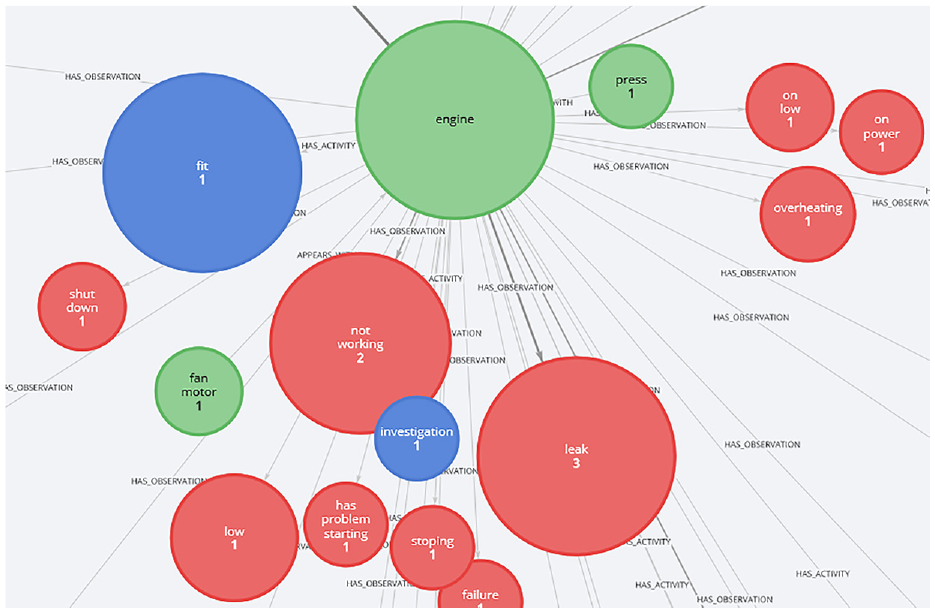
A screenshot from Echidna, where the user has clicked on the ‘engine’ node to show all entities related to engines and the number of times they co-occur.

Querying structured fields

The menu on the left enables users to query from across a range of different structured field types, such as dates, numerical values and categorical variables. These structured fields are taken from the input dataset. In the maintenance knowledge graph, for example, users may query the graph to return all nodes from work orders within a specific date range, cost range or work order type. Perhaps most notably is the ability to use this to search for specific functional locations (FLOCs), for example, ‘pumping systems’ or ‘engine lubrication system’, enabling reliability engineers the ability to rapidly drill down into their data and look at specific assets, as demonstrated in Figure 2.

Figure 2.

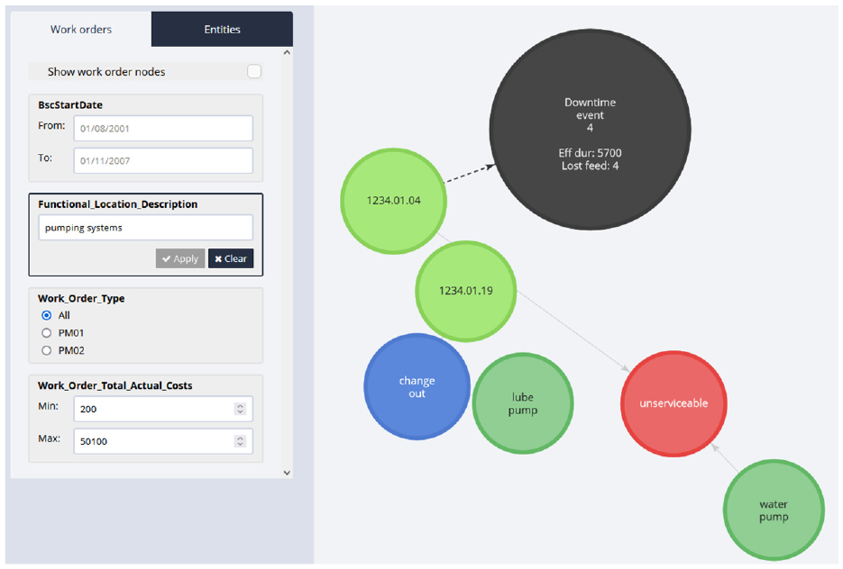
An example query result, where the user has entered ‘pumping systems’ into the functional location description search field.

Querying entities

The second tab of the left menu, ‘entities’, allows users to filtre the graph to show specific entity types. This enables users to centre the graph around particular asset types, that is, pumps, engines, air conditioners and so on, or on certain failure modes.

A notable feature is that this menu allows users to aggregate nodes from the same class together into a single node. For example, clicking the aggregation checkbox adjacent to the pump node as shown in Figure 3 will aggregate all pumps and all subclasses of pumps (sump pump, centrifugal pump, etc.) into one node. The user can then easily see the related activities and failure modes associated with all pumps appearing in the work orders.

Figure 3.

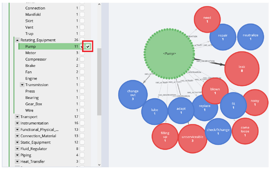
An example aggregation, where the user has elected to aggregate all ‘pumps’ and its subclasses into a single node. The aggregation checkbox is highlighted with a red box.

Grouping failure modes

The Observation nodes in the graph offer the most value to reliability engineers as they may be used for Failure Modes Effects Analysis (FMEA) and identifying unexpected failure modes. However, quite often the failure modes and what is written in the work orders by the maintainers differs – for example, maintainers often write ‘tripped’ as opposed to ‘electrical issue’, and ‘rusted’ rather than ‘structural deficiency’. In order to maximise the ability of Echidna to aid with failure mode effects analysis we have automatically grouped similar Observations together into specific failure mode categories, which were obtained from the ISO14224 (https://www.iso.org/standard/64076.html). The details of how this grouping is achieved is discussed in the following section. The grouping allows for all forms of a particular failure mode, for example, ‘tripped’, ‘low power’, ‘earth fault’ to be aggregated into a single node, allowing engineers to quickly view the number of times that particular failure mode has occurred on a piece of equipment.

Filtering by functional location

Another key feature of Echidna is the ability to filtre based on functional locations. Using the menu on the left, reliability engineers can drill down into the functional location hierarchy and quickly view a subgraph centred on particular functional location(s). This is most powerful when combined with the failure mode grouping and aggregation features, as it allows the user to view failure modes related to particular FLOCs and/or its subclasses. Figure 4 shows an example where the user has aggregated Electrical and Breakdowns into two single nodes, and has aggregated FLOC 1234.01 and its subclasses into a single node, in order to see that the FLOC experienced 19 electrical failures and 16 breakdowns.

Figure 4.

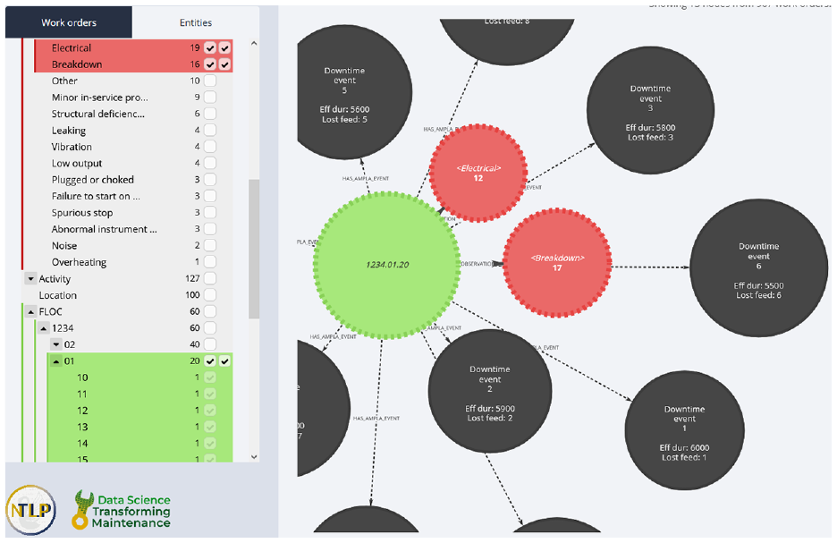
An example FLOC filtre, where the user has aggregated all FLOCs under ‘1234.01’ into a single node, and is viewing all Electrical and Breakdowns related to that FLOC and its subclasses.

Visualising downtime events

Echidna also possesses the ability to visualise downtime events. In the visualisation, downtime events are linked to the functional location for which the downtime was recorded. This enables reliability engineers with the ability to quickly view the number of times and the cost associated with particular pieces of equipment going down. This feature is further enhanced by the aforementioned aggregation system, allowing for a FLOC with several sub-FLOCs, each with downtime events, to be aggregated into a single node so that all downtime events pertaining to that FLOC and its sub-FLOCs are linked to a single node. This feature is also demonstrated in Figure 4.

MWO2KG – knowledge graph construction from technical short text

The following section describes MWO2KG, the pipeline through which the knowledge graph behind Echidna is constructed. MWO2KG, as shown in Figure 5, has been purpose-built for short technical text such as maintenance work orders. In contrast to Text2KG,³⁰ which is a rule-based system designed specifically for common corpora such as news reports, MWO2KG is a supervised-learning based model which allows it to construct knowledge graphs from any technical language domain so long as a set of annotated training data is provided to the model. Developers looking to deploy the software on other domains may freely modify MWO2KG’s pipeline to suit their needs, as it is separate from the Echidna web application.

Figure 5.

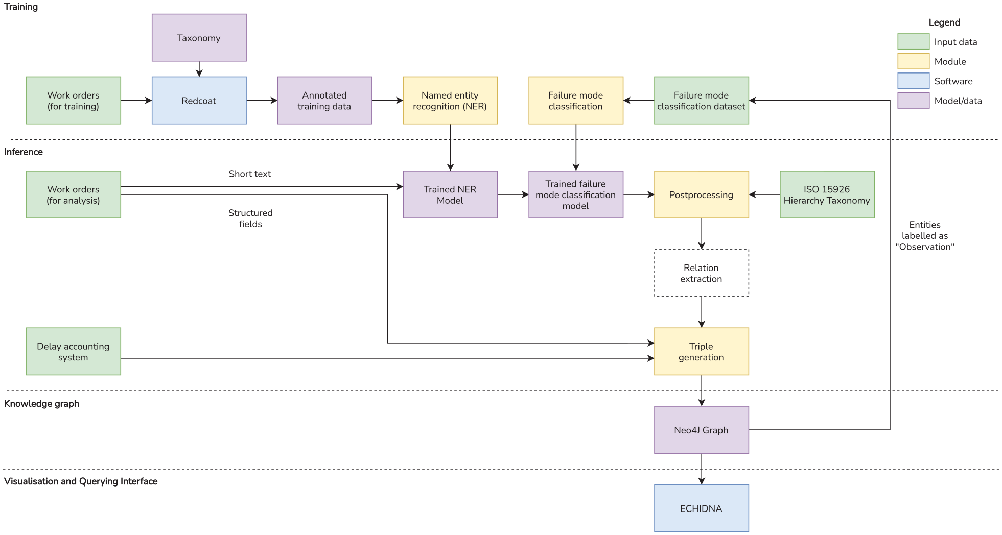
A block diagram of MWO2KG, which constructs a knowledge graph from technical short text such as maintenance work orders. Note that a ‘relation extraction’ step is not present in MWO2KG but has been included in the diagram for generalisation.

The pipeline is split into two distinct phases. The first phase is the training phase, where our deep learning model learns how to label the entities appearing in a set of maintenance work orders. This is accomplished via a set of manually-annotated training data. The second phase is the inference phase, where our trained deep learning model automatically labels a different set of work orders with the entities that appear in those work orders. These entities are then fed into the Postprocessing stage and are finally transformed into a knowledge graph via the Triple Generation stage.

Annotated data from Redcoat

The first stage of MWO2KG is therefore for the person deploying the pipeline (not necessarily the end user) to create or import a set of annotated work order data using Redcoat,²⁷ a web-based annotation tool for annotating textual data for machine learning. An example of three work orders that have been annotated in Redcoat is displayed in Figure 6. Users can import the short text field from a set of work orders into Redcoat and annotate them using one of the provided maintenance work order taxonomies, which contains a variety of important maintenance-specific entity types such as ‘item’, ‘activity’, ‘observation’ and ‘location’. The template also includes ‘metatags’, for example, ‘typo’ and ‘acronym’ which describe characteristics of the words themselves that are not related to entity types. These metatags are useful for other applications outside of MWO2KG, such as training models to detect abbreviations and to correct spelling errors.

Figure 6.

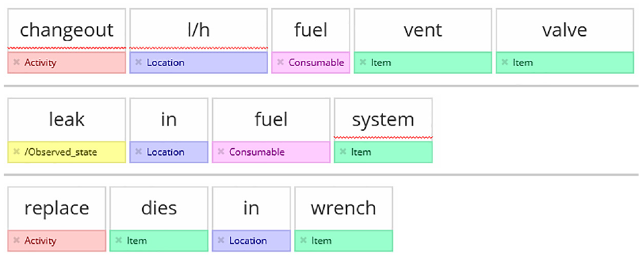
Three example work orders that have been annotated in Redcoat.

Once annotation in Redcoat is complete, the annotations can be exported from Redcoat and imported directly into the pipeline via a simple preprocessing script. This is necessary because annotations in Redcoat can have multiple labels per token, for example, ‘pmp’ is able to be labelled as both an ‘item’ and a ‘typo’. This is useful for entity typing models,³³ which can predict multiple labels per entity, but for the purposes of MWO2KG and Echidna we only require single labels per token. The annotations are therefore preprocessed so that each word has at most one label, that is, the first label assigned by the annotators that is an entity type (‘item’, ‘activity’) and not a metatag (‘typo’, ‘acronym’).

Named entity recognition

MWO2KG performs Named Entity Recognition (NER) in order to extract the entities appearing in the technical short text. NER is the process of automatically labelling each word in a sentence with its corresponding entity type.²² This task is performed in two stages. The first stage is the training stage, where the model learns how to predict labels correctly by training on the annotated training data. The second stage is the analysis phase, where the trained model predicts the labels on previously unseen data (in our case, a second set of analysis work orders).

Before a sentence can be fed into a NER model, it must first be converted to word embeddings. Word embeddings, which are numerical representations of words, are a crucial factor in the high performance of NLP models.³⁴ Word embeddings are produced by language models, which fall under three categories: word-level, wordpiece-level, and character-level. Word-level language models, such as Word2Vec,³⁵ aim to compute one embedding vector per word, that is, ‘pump’ and ‘pmp’ will each have two separate vectors. Wordpiece-level language models, such as BERT,³⁶ split words into smaller fragments (wordpieces), and compute embeddings for each wordpiece. For example, ‘pump’ might be split into ‘pu’ and ‘mp’, and ‘pmp’ into ‘p’ and ‘mp’. This allows for a greater ability to compute embeddings for previously unseen words, as some wordpieces in those words may have already been seen by the model. Character-level language models, on the other hand, compute embeddings based on the characters appearing in each word.³⁷ This makes character-level language models adept at handling minor lexical variations in words (such as spelling errors and abbreviations) which are rife in technical short text.

In MWO2KG the Named Entity Recognition task is therefore performed using Flair,³⁸ a popular open source natural language processing library supporting a wide range of tasks (https://github.com/flairNLP/flair). Flair provides the ability to train and evaluate named entity recognition models and incorporates a high quality pretrained character-level language model with which to compute embeddings.

Similarly to most deep learning-based architectures for natural language processing, the Flair sequence labelling model is comprised of three interconnected layers. The first layer is an embedding layer, which serves to embed each of the input characters into numerical vector representations. As our dataset is too small to train embeddings on (most language models are trained on billions of words), we use pretrained Flair embeddings (‘mix-forward’ and ‘mix-backward’), which have been trained on a mix of common corpora such as web crawls and Wikipedia. These embeddings are fed through a bidirectional long short-term memory (LSTM) layer, which encodes the contextual information of each word. The outputs of the LSTM layer are fed to a softmax layer which predicts the most likely class label for each word in the input sentence. The model is optimised using the stochastic gradient descent (SGD) algorithm to perform backpropagation.

Failure mode classification

The aim of the failure mode classification stage is to group similar failure modes together. For example, ‘rusted’, ‘corroded’, ‘wear’ are all examples of structural deficiency and should be grouped as such by adding a label named ‘structural_deficiency’ to each node. The failure mode classification stage does this grouping automatically using text classification, a natural language processing task that takes a sentence as input, and classifies the sentence with a single label.³⁹ In this case the input is a single ‘observation’ (as classified by the Named Entity Recognition model), and the output is a structured failure mode code such as ‘spurious stop’, ‘high output’ and ‘breakdown’. The model itself is once again implemented using the Flair library, this time using the text classification model. This is essentially identical to Flair’s sequence labelling model, but rather than predicting a label for each word, it instead predicts a label for each sentence.

Training the model requires an annotated dataset of (observation, failure mode code) pairs. The list of observations can be easily obtained by querying the Neo4j graph, which can be built without failure mode classification enabled in the first instance. The observations must then be labelled with their corresponding failure mode code and fed into the model for training. As part of this work we developed an annotated dataset of approximately 1000 (observation, failure mode code) pairs, where the set of failure mode codes was taken from the ISO 14224. In order to ensure a sufficiently small set of classes we condensed the ISO 14224 codes into a set of 19 codes, and each observation was labelled with the most relevant class in this set.

Postprocessing

The aim of the first stage of the postprocessing step is to incorporate real-world asset hierarchies into the final knowledge graph. In the previous stage, the Named Entity Recognition model labels each asset with only one label, that is, the ‘item’ label. In order to facilitate more useful filtering in the Echidna visualisation, the postprocessing step of MWO2KG automatically labels any entities labelled as ‘item’ with a list of asset classes based on the ISO 15926 asset hierarchy taxonomy.⁴⁰ For example, ‘pump’ is assigned the labels ‘rotating equipment’ and ‘pump’. This step is not performed using machine learning but rather via a rule-based approach. If the name of the entity (e.g. ‘pump’) appears in the ISO 15926, it is also assigned with all parents of that asset class according to the taxonomy.

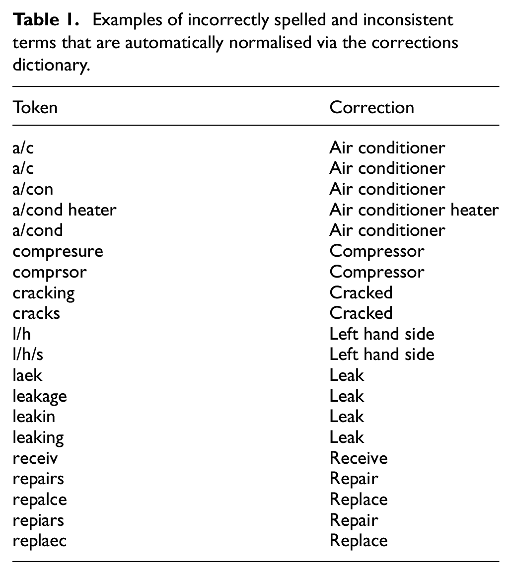
The second and final stage of the postprocessing step is to automatically normalise any incorrectly spelled or inconsistently named entities prior to their insertion into the knowledge graph. This is necessary because the NER model will occasionally mispredict entity labels, or the spelling of certain entities will be inconsistent across the dataset (i.e. ‘pump’ might be spelled as ‘pmp’, ‘puump’ and so on). The normalisation step resolves similar entity names into a single node, fortifying the accuracy of the knowledge graph.

This step is accomplished using a dictionary of (word, normalised word) pairs. A list of example terms from this dictionary are shown in Table 1. The dictionary currently contains 140 manually-curated correction pairs, which can be easily expanded by the user as necessary. The user can easily create this list after running the pipeline once, by using Echidna to visualise a list of entities the model predicted and adding the misspelled entities and their respective corrections to a list. Alternatively, lexical normalisation tools such as Lexiclean⁴¹ can be used to automatically clean the data prior to running the pipeline, removing the need to create a dictionary.

Table 1.

Examples of incorrectly spelled and inconsistent terms that are automatically normalised via the corrections dictionary.

Token	Correction
a/c	Air conditioner
a/c	Air conditioner
a/con	Air conditioner
a/cond heater	Air conditioner heater
a/cond	Air conditioner
compresure	Compressor
comprsor	Compressor
cracking	Cracked
cracks	Cracked
l/h	Left hand side
l/h/s	Left hand side
laek	Leak
leakage	Leak
leakin	Leak
leaking	Leak
receiv	Receive
repairs	Repair
repalce	Replace
repiars	Repair
replaec	Replace

Triple generation

The last stage of MWO2KG is to create a set of triples and import these triples into the knowledge graph. A triple is a data structure with three components: a head entity, a tail entity and a relation. The head entity is linked to the tail through the relation. For example, ‘pump’ is linked to ‘leak’ through the ‘has_observation’ relation.

The triple generation stage takes each predicted entity in a work order and links them to one another through the appropriate relation. Rather than perform this task using the traditional method of ‘relation extraction’,²⁶ which involves supervised learning and hence another training dataset, MWO2KG adopts a heuristics-based method that automatically builds relationships between every entity labelled as an ‘item’ and every other entity appearing in the same work order. This method is particularly well suited to technical short text as it is typically very short (5–8 words) and in the overwhelming majority of cases, the entities surrounding an item are related to that item.

Lastly, MWO2KG incorporates structured data from two additional sources: functional locations (FLOCs) and Downtime Events. The triple generation stage constructs nodes from the functional locations listed in the work order dataset, and links those functional locations to every entity appearing in the corresponding work order. FLOC nodes are therefore similar to item nodes but represent a specific asset rather than a class of assets, for example, ‘pump’. Downtime events may also optionally be incorporated into the graph in this stage, if the user has such a dataset available. The downtime events are linked to the FLOC listed in the FLOC column of the downtime event, and are assigned node properties based on their effective cost and duration.

Once all of the triples have been built, they are imported into Neo4j (https://neo4j.com/), a graph database management system that supports graph-based queries through the Cypher query language. The Neo4j-based graph can be queried through the Neo4j interface or through our Echidna visualisation.

Experiments

Due to the novelty of constructing knowledge graphs from maintenance work orders and the lack of available baseline datasets, it is not possible to quantitatively analyse the performance of the pipeline as a whole. We therefore carry out two experiments in order to determine the performance of two components of MWO2KG: the Named Entity Recognition component and the Failure Mode Classification component.

Metrics

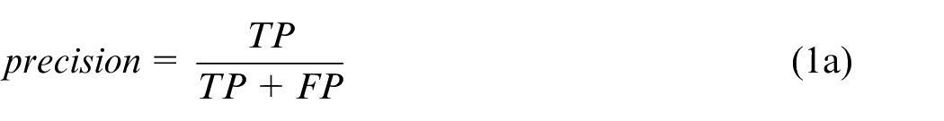
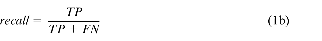
We evaluate the performance of our model using F1-score (also known as F-score), which is calculated from the precision and recall of a test. For each class label, precision and recall are calculated based on true positives (TP), false positives (FP) and false negatives (FN):

precision = \frac{TP}{TP + FP}

(1a)

recall = \frac{TP}{TP + FN}

(1b)

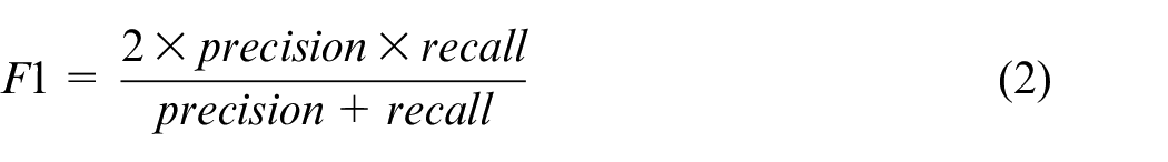
The F1-Score for each class label is calculated as follows:

F 1 = \frac{2 \times precision \times recall}{precision + recall}

(2)

In order to evaluate the performance across every class label, we use two additional metrics: Micro F1 and Macro F1. Micro F1 calculates an F1-Score by adding the TPs, FPs and FNs from all class labels together and then calculating F1-Score:

MicroF 1 = F 1_{(class 1 + class 2 + \dots + classn)}

(3)

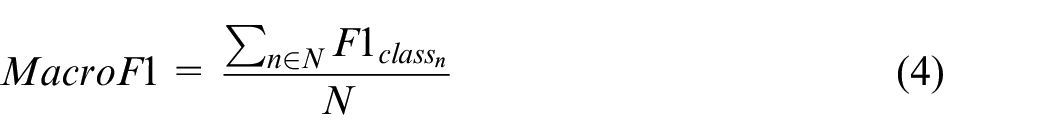
Macro-F1, on the other hand, simply averages the F1-Score of each class. Given N is the number of class labels, it is calculated as follows:

MacroF 1 = \frac{\sum_{n \in N} F 1_{clas s_{n}}}{N}

(4)

Datasets

The dataset used to train and evaluate the Named Entity Recognition model comprises 3200 work orders (for training), 401 work orders (for validation) and 401 work orders (for testing). These work orders were manually annotated by a team of 10 annotators from our research group, the University of Western Australia Natural and Technical Language Processing Group (https://nlp-tlp.org/). The dataset features 10 entity types in total, capturing a range of maintenance-specific concepts such as items, activities, consumables and locations. We plan to discuss this dataset in significantly more detail and release the dataset in a future paper.

The dataset used to train and evaluate the Failure Mode Classification model comprises 502 (observation, label) pairs (for training), 62 pairs (for validation) and 62 pairs (for testing). The labels are taken from a set of 22 failure mode codes from ISO 14224. In order to pull a list of observations in which to label, we ran MWO2KG over the data once and exported a list of all entities labelled as ‘observation’ (such as ‘leaking’, ‘not working’) by the Named Entity Recognition model. We then removed all results that were incorrectly predicted as observations by the NER model and proceeded to label each observation with the most appropriate failure mode code using a text editor.

Finally, we upsampled the minority classes in the training dataset in an attempt to alleviate class imbalance issues. The upsampling process involved repeating each sample such that each of the failure mode code classes had the same number of samples in the training set. While the upsampling approach taken was relatively simplistic, we found it was the best way to ensure that the model did not overfit to the most common class (‘minor in-service problems’). A more sophisticated upsampling method such as SMOTE (Synthetic Minority Oversampling TEchnique)⁴² may improve the process by generating similar words (by sampling the vector space between the embeddings of two given words), rather than repeat the same words multiple times in the training set. However, this would require manual curation to ensure the generated words are valid, and is outside the scope of this paper.

Results

In this section we aim to determine the performance of MWO2KG in order to determine its effectiveness in constructing knowledge graphs from maintenance work orders. More specifically we aim to address the two following criteria:

How well does the Named Entity Recognition model label entities from work orders it has not seen before?

How well does the Failure Mode Classification model classify an observation into a failure mode code?

Named entity recognition results

The results of the Named Entity Recognition (NER) model are shown in Table 2. Overall the scores are high considering the substantial challenges involved in technical language processing, such as acronyms, domain-specific jargon and spelling errors. Micro-F1 and Macro-F1 scores of 0.828 and 0.858 respectively suggest that NER component is scalable to large volumes of unseen work order data and is fit for purpose. For comparison, the current state-of-the-art NER models in natural language processing research achieve slightly higher F1-Scores in the vicinity of 0.90–0.94,^43,44 which is unsurprising given that the news report data on which these models were trained is clean, grammatically-correct and generally free of the wide range of challenges present in technical language. The fact that our models are achieving relatively similar performance to these state-of-the-art models that were trained and evaluated on clean data is a testament to the quality of the model as well as our dataset.

Table 2.

The results of the Named Entity Recognition model on the test dataset.

Entity class	Sup.	Precision	Recall	F1-Score
Activity	199	0.909	0.900	0.904
Agent	29	0.829	1.000	0.906
Attribute	12	0.615	0.667	0.64
Cardinality	17	0.882	0.882	0.882
Consumable	42	0.800	0.857	0.828
Item	520	0.767	0.825	0.795
Location	135	0.815	0.882	0.847
Observation	199	0.807	0.799	0.803
Specifier	10	1.000	1.000	1.000
Time	17	1.000	0.941	0.970
Micro-F1				0.828
Macro-F1				0.858

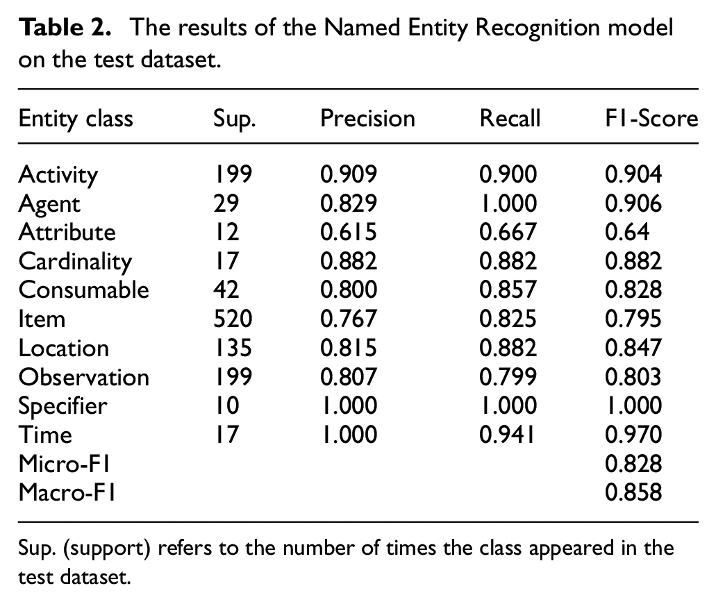
Sup. (support) refers to the number of times the class appeared in the test dataset.

Further insight into the predictive capability of our model is provided in Table 3, which shows three example sentences that have been labelled by the NER model. The correct labels (i.e. the ground truth) are displayed in the rightmost column. The first sentence, ‘blowen hyd hose on bottem of mast’, demonstrates the noise prevalent in maintenance work orders – in this case, there are two spelling errors (‘blowen and bottem’) and one abbreviated term (‘hyd’). The NER model correctly understood that ‘blowen’ is meant to be ‘blown’ (and hence an observation), but could not correctly identify that ‘bottem’ was meant to be part of the trigram ‘on bottom of’ (a Location).

Table 3.

Three example sentences from the test set that were tagged by the NER model.

Token	Predicted label	Correct label
blowen	B-Observation	B-Observation
hyd	B-Item	B-Item
hose	I-Item	I-Item
on	B-Location	B-Location
bottem	B-Item	I-Location
of	O	I-Location
mast	B-Item	I-Item
warr	B-Agent	O
:	O	O
cabin	B-Item	B-Item
&	O	O
air	B-Item	B-Item
pipe	I-Item	I-Item
suport	B-Item	B-Item
damage	B-Observation	B-Observation
replace	B-Activity	B-Activity
chip	B-Item	B-Item
deflector	I-Item	I-Item
&	O	O
deck	B-Item	B-Item
seal	B-Item	B-Item
l	B-Location	O

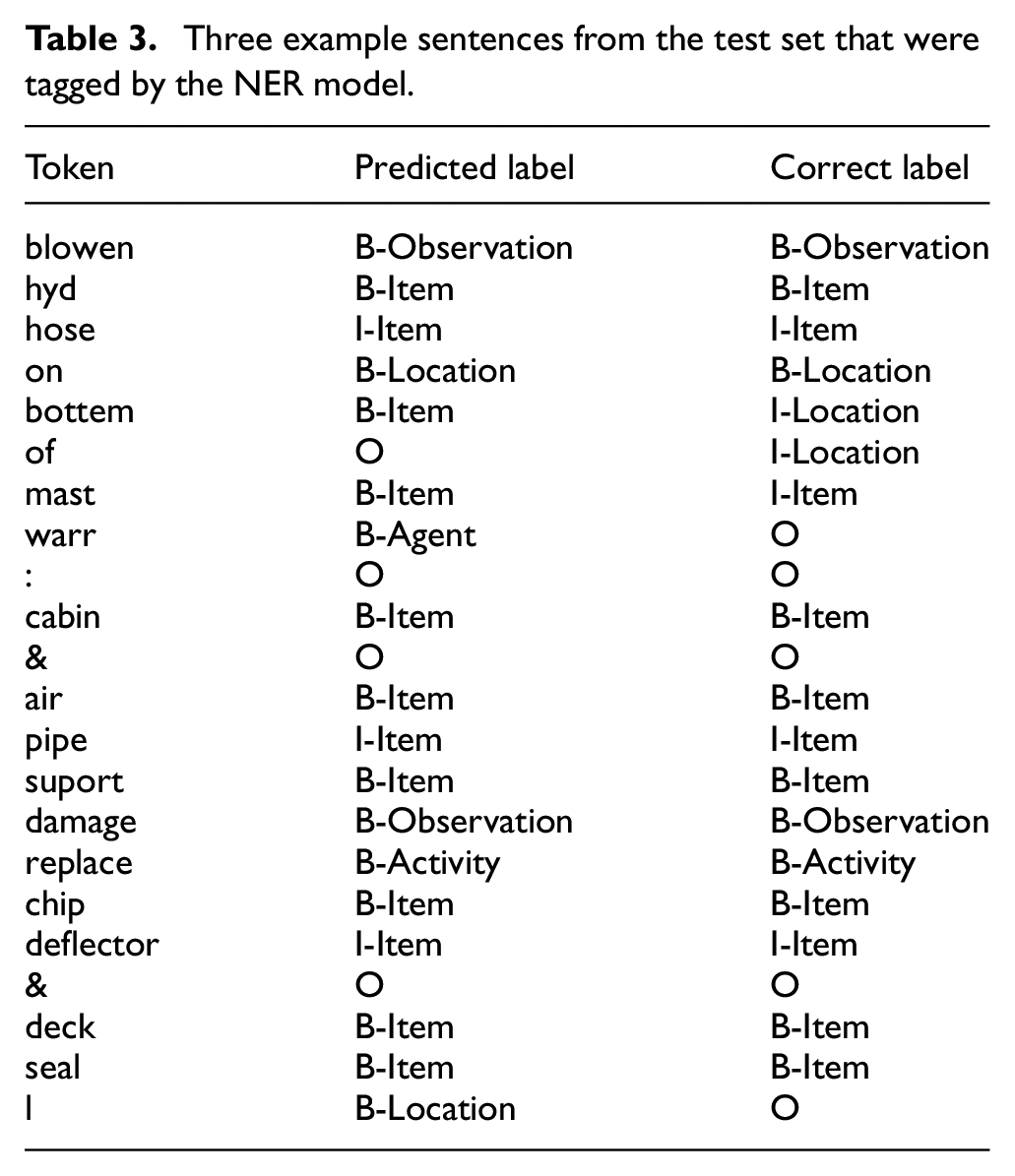
The second sentence, ‘warr : cabin & air pipe suport damage’, presents an interesting case: ‘warr’ (short for ‘warranty’) is a token that rarely appears in our dataset (five times in the test dataset in the form of ‘warr’, and three as ‘warranty’). It does not belong to any entity class, however – our group made the conscious decision not to develop a particular entity class for it as such a class would only contain that one single term. Our model therefore had difficulty understanding that it was meant to be left untagged. Of the five times ‘warr’ appeared in the test dataset, our model tagged it as Agent three times and Item twice, and it tagged ‘warranty’ as Activity twice and O (no entity class) once.

The third and final sentence in Table 3, ‘replace chip deflector & deck seal l’ demonstrates another interesting case. The term ‘l’ was identified by our model as a Location (presumably because it is commonly used to denote ‘left’), however in our ground truth set we elected not to label it, as we thought it was an example of trailing noise at the end of the work order. It is possible that our ground truth is actually incorrect in this instance, though. If the sentence was written in regular English, then it would not be grammatically possible for ‘l’ to mean ‘left’ in this case, but maintenance work orders are often terse and words are not necessarily always in the correct grammatical order. The term ‘l’ here could be referring to the deck seal in the leftmost position, meaning that despite the model getting it ‘wrong’ according to our ground truth, there is an argument to be made that the model is actually correct here.

It is worth noting that the results of the NER model do not necessarily provide an indication of how accurately the Triple Generation step is able to automatically create links between entities in the work orders when constructing the graph. Our experience is that the short length of each work order resulted in highly accurate connections between entities, however for larger datasets a more thorough performance analysis of the triple generation step would be worthwhile in order to determine whether a more sophisticated relation extraction model should be used instead.

Failure mode classification results

The results of the failure more classification model are displayed in Table 4. Overall, the model was proficient at tagging some classes, such as ‘structural deficiency’, ‘Minor in-service problems’, ‘leaking’ and ‘overheating’. These classes tended to contain a well-defined, semantically-similar list of terms (e.g. ‘hot’, ‘smoking up’, ‘smoking hot’, etc. for overheating, and ‘cracked’, ‘rusted’, etc. for structural deficiency). Moreover, these classes are semantically distinct from the other classes, avoiding the possibility of the model selecting a similar class instead of the correct class. This is in contrast to some of the other more ambiguous classes –‘Breakdown’ and ‘Failure to start on demand’– which are semantically similar and thus difficult for the model to differentiate.

Table 4.

The precision, recall and F1-scores of the failure mode classification model across each of the failure mode classes appearing in the test dataset. Note that four classes were not present in the test data and hence not listed in the table.

Failure mode	Support	Precision	Recall	F1-Score
Breakdown	7	0.333	0.429	0.375
Plugged/choked	6	0.667	0.667	0.667
Leaking	3	0.667	0.667	0.667
Minor in-service problems	17	0.846	0.647	0.733
Structural deficiency	3	0.429	1.000	0.600
Failure to start on demand	1	0.250	1.000	0.400
Vibration	2	1.000	0.500	0.667
Overheating	4	1.000	1.000	1.000
Fail to function	3	1.000	0.333	0.500
Low output	2	0.000	0.000	0.000
Electrical	6	0.667	0.667	0.667
Failure to stop on demand	1	0.000	0.000	0.000
Abnormal instrument reading	1	1.000	1.000	1.000
Other	2	1.000	0.500	0.667
Contamination	1	1.000	1.000	1.000
High output	1	0.000	0.000	0.000
Erratic output	1	0.000	0.000	0.000
Spurious stop	1	0.000	0.000	0.000
Micro-F1				0.597
Macro-F1				0.459

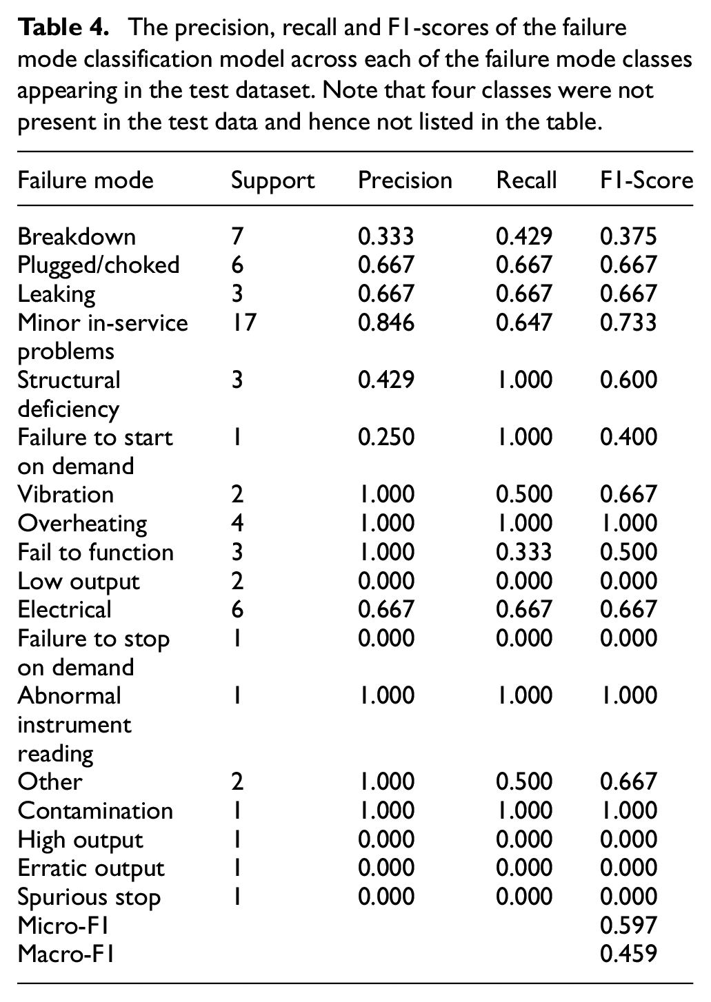
There are two other reasons that the model did not fair as well on the other classes. The first is due to the low quality of the ground truth set. It is difficult for human annotators to consistently label individual words with their corresponding failure mode, as many words could be considered to belong to multiple categories (e.g. is ‘fault’ an electrical issue, failure to function or a breakdown?). Our annotators were as consistent as possible, but unlike the 4002 work order Named Entity Recognition dataset, which was developed over a year of annotation, the Failure Mode Classification dataset was constructed relatively quickly and with little prior experience. The ground truth set is therefore ‘noisy’ when compared to the ground truth set of the named entity recognition task.

Secondly, the training dataset only contains 502 (observation, label) pairs, which is simply not enough to train a model to accurately predict minority classes even after upsampling the minority classes in the training data. We are optimistic, however, that with further work on refining the model and with additional annotation, our Failure Mode Classification will exhibit similar performance to the Named Entity Recognition model in future. In its current state the model still provides, to the best of our knowledge, the first approach to failure mode classification from technical short text and therefore represents significant value to reliability engineers.

In order to further elucidate the model’s performance, a list of predictions made by the model on the test set are demonstrated in Table 5. The table shows 14 examples taken from the test set (which contains a total of 62 records). The first seven examples are phrases that were correctly labelled by the model, that is, the prediction matched the ground truth label assigned by the human annotators. These examples showcase the model’s ability to make confident predictions about several of the majority classes, for example, ‘Electrical’, ‘Breakdown’ and ‘Leaking’. These examples also highlight the model’s ability to deal with noise in the input phrases. For example, the model correctly identified that ‘vibrationlubealignment’ had the failure mode code of ‘Vibration’ despite the lack of spaces. The model was even able to correctly label ‘require tighteninginspecti’ despite the missing space and poor spelling. Another example is ‘not truning’, a misspelling that was correctly labelled by the model as ‘Plugged/choked’. The model is able to deal with these issues because it is trained at the character-level, and is hence able to handle minor variations in spelling and a lack of spacing between words.

Table 5.

Ten example phrases tagged by the failure mode classification model, showing the ground truth, prediction by the model and the model’s confidence in making that prediction.

Phrase	Ground truth	Prediction	Confidence
doesnt trip	Electrical	Electrical	0.987
has failed	Breakdown	Breakdown	0.958
spraying out slurry	Leaking	Leaking	0.948
not truning	Plugged/choked	Plugged/choked	0.556
hot joint	Overheating	Overheating	0.744
vibrationlubealignment	Vibration	Vibration	0.814
require tighteninginspecti	Minor in-service problems	Minor in-service problems	0.959
sticking shu	Fail to function	Failure to stop on demand	0.299
does not work	Breakdown	Failure to start on demand	0.468
runs continuously	Failure to stop on demand	Spurious stop	0.532
unable to pump	Low output	Plugged/choked	0.939
surging cutting in and out	Electrical	Erratic output	0.680
requires rebuild	Minor in-service problems	Breakdown	0.751
burst	Breakdown	Structural deficiency	0.892

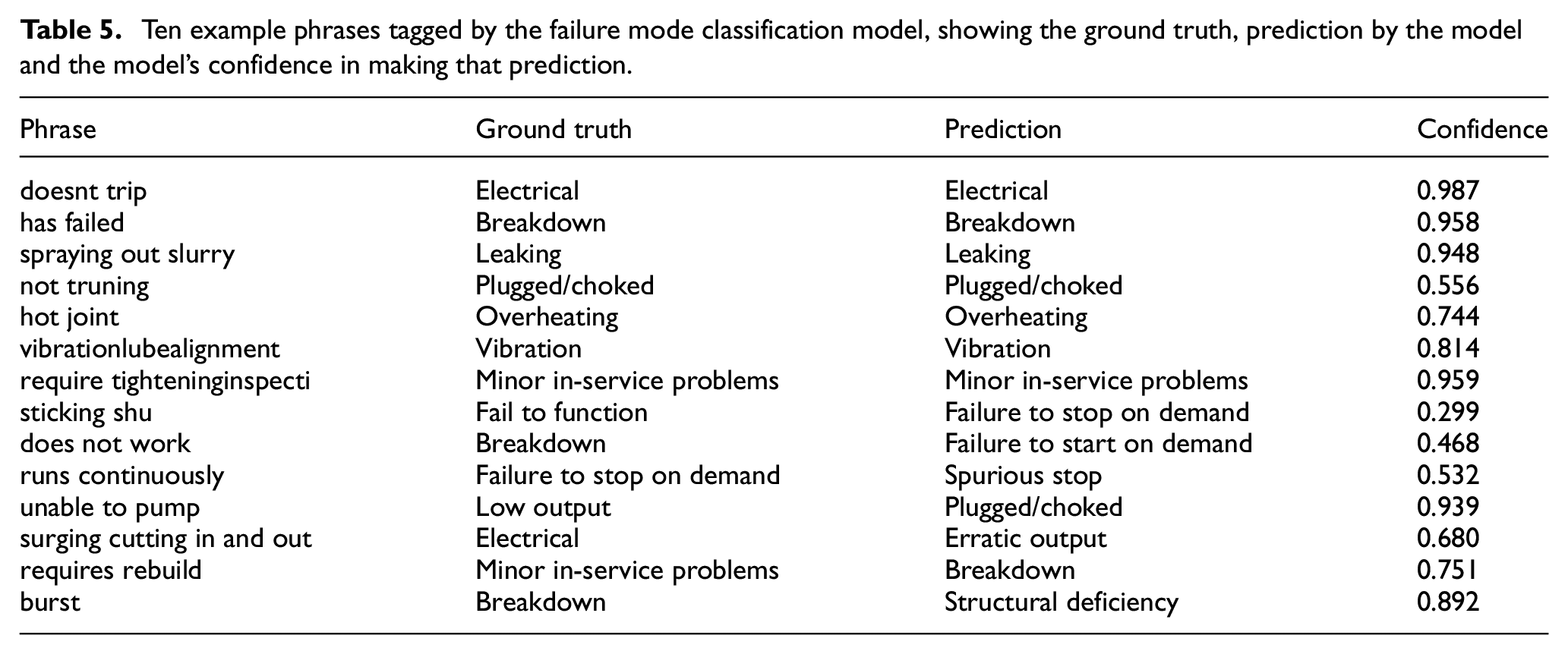
The last seven examples are phrases that were incorrectly labelled by the model. Many of the errors made by the model are minor, in that the class label predicted by the model is highly similar to the class label of the ground truth. For example, the model labelled ‘does not work’ as a ‘failure to start on demand’ rather than a ‘breakdown’, but one could argue that both labels are actually valid for this example. A human might label ‘does not work’ as either one of these labels, considering they both make sense in this context. Similarly, ‘unable to pump’ was labelled as ‘pumped/choked’ rather than ‘low output’, which could also be considered correct. There are of course other examples where the model completely failed to label the training examples correctly –‘runs continuously’ being labelled as ‘spurious stop’ being the most egregious – but in general the erroneous predictions made tend to be quite close to the ground truth labels.

Conclusion and future work

In this paper we have presented a software system for visualising knowledge graphs built from technical short text: Echidna, a web-based interface for visualising and querying a maintenance knowledge graph, and MWO2KG, a pipeline for constructing knowledge graphs from technical short text. Together these tools represent a novel methodology for analysing work orders and demonstrate the effectiveness of technical language processing in maximising decision support for reliability engineers. The tools provide reliability engineers with a powerful new way to visualise historic asset data and easily identify failure modes.

In future we aim to further improve the tool by allowing data owners to upload their own datasets without needing to run MWO2KG programmatically. At present only one graph can be visualised by Echidna at a time, so we are working on the ability to store and visualise multiple graphs. This will allow reliability engineers from across multiple locations in an organisation to access and utilise their respective knowledge graphs simultaneously. We also aim to continue working on improving the failure mode classification model and creating a larger training dataset in order to more accurately group technical language observations into structured failure mode codes.

Footnotes

Declaration of conflicting interests

The author(s) declared no potential conflicts of interest with respect to the research, authorship, and/or publication of this article.

Funding

The author(s) disclosed receipt of the following financial support for the research, authorship, and/or publication of this article: This research is supported by the Australian Research Council through the Centre for Transforming Maintenance through Data Science (Grant Number IC180100030), funded by the Australian Government. Additionally, Hodkiewicz acknowledges funding from the BHP Fellowship for Engineering for Remote Operations. Liu acknowledges funding from the Australian Research Council Discovery Grant DP150102405.

ORCID iDs

Michael Stewart

Melinda Hodkiewicz

References

Klyne

Carroll

McBride

Resource description framework (rdf): concepts and abstract syntax, http://www.w3.org/TR/2004/REC-rdf-concepts-20040210 (2004, accessed September 2021).

Cyganiak

Wood

Lanthaler

, et al. RDF 1.1 concepts and abstract syntax. http://www.w3.org/TR/2014/REC-rdf11-concepts-20140225. (accessed September 2021)

Strötgen

Tran

Friedrich

, et al. Towards the Bosch materials science knowledge base. In: International semantic web conference, Auckland, New Zealand, 2019.

Noy

Gao

Jain

, et al. Industry-scale knowledge graphs: Lessons and challenges. Queue 2019; 17(2): 48–75.

Levesque

HJ.

Knowledge representation and reasoning. Annu Rev Comput Sci 1986; 1(1): 255–287.

Lakemeyer

Nebel

Foundations of knowledge representation and reasoning. Springer, Vienna, Austria, 1994, pp.1–12.

Hubauer

Lamparter

Haase

, et al. Use cases of the industrial knowledge graph at siemens. In: International semantic web conference, P&D/Industry/BlueSky, Monterey, CA, 2018.

Liebig

Maisenbacher

Opitz

, et al. Building a knowledge graph for products and solutions in the automation industry. 2019. https://openreview.net/pdf?id=ByldIMlEDV (accessed 1 September 2021).

Aliyu

A. F. D

Aliyu

Development of knowledge graph for university courses management. Int J Educ Manag Eng 2020; 10(2): 1–10.

10.

Nguyen

Kertkeidkachorn

Ichise

, et al. Mtab: matching tabular data to knowledge graph using probability models. arXiv preprint arXiv:191000246, 2019.

11.

Elfaki

Aljaedi

Duan

. Mapping erd to knowledge graph. In: 2019 IEEE World Congress on Services (SERVICES), Beijing, China, 2020, vol. 2642, pp. 110–114. IEEE.

12.

Brundage

Sexton

Hodkiewicz

, et al. Technical language processing: unlocking maintenance knowledge. Manuf Lett 2021; 27: 42–46.

13.

Dima

Lukens

Hodkiewicz

, et al. Adapting natural language processing for technical text. Applied AI Letters 2021; 2: e33.

14.

Liu

Boyd

, et al. Identifying causality and contributory factors of pipeline incidents by employing natural language processing and text mining techniques. Process Saf Environ Prot 2021; 152: 37–46.

15.

Yang

Baraldi

Zio

A novel method for maintenance record clustering and its application to a case study of maintenance optimization. Reliab Eng Syst Saf 2020; 203: 107103.

16.

Suh

Sectoral patterns of accident process for occupational safety using narrative texts of OSHA database. Saf Sci 2021; 142: 105363.

17.

Macêdo

das Chagas Moura

Aichele

, et al. Identification of risk features using text mining and Bert-based models: application to an oil refinery. Process Saf Environ Prot 2022; 158: 382–399.

18.

Boggs

Wali

Khattak

AJ.

Exploratory analysis of automated vehicle crashes in California: a text analytics & hierarchical Bayesian heterogeneity-based approach. Accid Anal Prev 2020; 135: 105354.

19.

Martinez-Rodriguez

Lopez-Arevalo

Rios-Alvarado

AB.

OpenIE-based approach for knowledge graph construction from text. Expert Syst Appl 2018; 113: 339–355.

20.

Mehta

Singhal

Karlapalem

. Scalable knowledge graph construction over text using deep learning based predicate mapping. In: Companion proceedings of the 2019 world wide web conference, San Francisco, CA, 2019, pp. 705–713. ACM.

21.

Stewart

Liu

. Seq2KG: an end-to-end neural model for domain agnostic knowledge graph (not text graph) construction from text. In: Proceedings of the 17th international conference on principles of knowledge representation and reasoning, Rhodes, Greece, 2020, pp. 748–757.

22.

Nadeau

Sekine

A survey of named entity recognition and classification. Lingvist Investig 2007; 30(1): 3–26.

23.

Gao

Woods

Liu

, et al. Pipeline for machine reading of unstructured maintenance work order records. In: Proceedings of the 30th European safety and reliability conference and 15th probabilistic safety assessment and management conference, Venice, Italy, 2020.

24.

Sexton

Brundage

MP.

Nestor: a tool for natural language annotation of short texts. J Res Natl Inst Stand Technol 2019; 124: 1–5.

25.

Ottermo

Håbrekke

Hauge

, et al. Technical language processing for efficient classification of failure events for safety critical equipment. In: PHM Society European conference, Virtual (online), 2021, vol. 6, pp. 1–9.

26.

Pawar

Palshikar

Bhattacharyya

Relation extraction: a survey. arXiv preprint arXiv:171205191, 2017.

27.

Stewart

Liu

Cardell-Oliver

. Redcoat: a collaborative annotation tool for hierarchical entity typing. In: Proceedings of the 2019 conference on empirical methods in natural language processing and the 9th international joint conference on natural language processing (EMNLP-IJCNLP): system demonstrations, Hong Kong, China, 2019, pp. 193–198.

28.

Hastings

Sexton

Brundage

, et al. Agreement behavior of isolated annotators for maintenance work-order data mining. In: Proceedings of the annual conference of the prognostics and health management society, Scottsdale, AZ, USA, 2019, pp. 1–7.

29.

Huang

Zhang

, et al. Knowledge graph embedding based question answering. In: Proceedings of the twelfth ACM international conference on web search and data mining, Melbourne, VIC, Australia, 2019, pp. 105–113.

30.

Stewart

Enkhsaikhan

Liu

ICDM 2019 knowledge graph contest: team UWA. In: Proceedings of the 2019 IEEE international conference on data mining (ICDM), Beijing, China, 2019, pp. 1546–1551. IEEE.

31.

Fricke

Semantic scholar. J Med Libr Assoc 2018; 106(1): 145.

32.

Hodkiewicz

Batsioudis

Radomiljac

, et al. Why autonomous assets are good for reliability–the impact of ‘operator-related component’failures on heavy mobile equipment reliability. In: Annual conference of the PHM Society, St. Petersburg, FL, 2017, vol. 9.

33.

Stewart

Liu

E2eet: from pipeline to end-to-end entity typing via transformer-based embeddings. arXiv preprint arXiv:200310097, 2020.

34.

Chen

Perozzi

Al-Rfou

, et al. The expressive power of word embeddings. arXiv preprint arXiv: 13013226, 2013.

35.

Mikolov

Sutskever

Chen

, et al. Distributed representations of words and phrases and their compositionality. In: Burges

CJC

Bottou

Welling

, et al. (eds.) Advances in neural information processing systems. Curran Associates Inc., Lake Tahoe, Nevada, 2013, pp. 3111–3119.

36.

Devlin

Chang

Lee

, et al. Bert: Pre-training of deep bidirectional transformers for language understanding. arXiv preprint arXiv:181004805, 2018.

37.

Akbik

Blythe

Vollgraf

. Contextual string embeddings for sequence labeling. In: Proceedings of the 27th international conference on computational linguistics, Santa Fe, NM, USA, 2018, pp. 1638–1649. Association for Computational Linguistics.

38.

Akbik

Bergmann

Blythe

, et al. Flair: an easy-to-use framework for state-of-the-art nlp. In: Proceedings of the 2019 conference of the North American chapter of the association for computational linguistics (demonstrations), Minneapolis, MN, USA, 2019, pp. 54–59.

39.

Schröder

Niekler

A survey of active learning for text classification using deep neural networks. arXiv preprint arXiv:200807267, 2020.

40.

Leal

ISO 15926 “Life cycle data for process plant”: an overview. Oil & gas science and technology 2005; 60(4): 629–637.

41.

Bikaun

French

Hodkiewicz

, et al. LexiClean: an annotation tool for rapid multi-task lexical normalisation. In Proceedings of the 2021 conference on empirical methods in natural language processing: system demonstrations, Online and Punta Cana, Dominican Republic, 2021, pp. 212–219. Association for Computational Linguistics.

42.

Chawla

Bowyer

Hall

, et al. Smote: synthetic minority over-sampling technique. J Artif Intell Res 2002; 16: 321–357.

43.

Yamada

Asai

Shindo

, et al. LUKE: deep contextualized entity representations with entity-aware self-attention. In: Proceedings of the 2020 conference on empirical methods in natural language processing (EMNLP), online, 2020, pp. 6442–6454. Association for Computational Linguistics.

44.

Bohnet

Poesio

Named entity recognition as dependency parsing. arXiv preprint arXiv:200507150, 2020.

MWO2KG and Echidna: Constructing and exploring knowledge graphs from maintenance data

Abstract

Keywords

Introduction

Related work

Echidna – an interactive knowledge graph visualisation and query interface for technical text

Nodes and edges

User interaction

Querying structured fields

Querying entities

Grouping failure modes

Filtering by functional location

Visualising downtime events

MWO2KG – knowledge graph construction from technical short text

Annotated data from Redcoat

Named entity recognition

Failure mode classification

Postprocessing

Triple generation

Experiments

Metrics

Datasets

Results

Named entity recognition results

Failure mode classification results

Conclusion and future work

Footnotes

Declaration of conflicting interests

Funding

ORCID iDs

References