Sage Journals: Discover world-class research

Abstract

A major part of Prognostic and Health Management of rotating machines is dedicated to diagnosis operations. This makes early and accurate diagnosis of single and multiple faults an economically important requirement of many industries. With the well-known challenges of multiple faults, this paper proposes a new Blended Ensemble Convolutional Neural Network – Support Vector Machine (BECNN-SVM) model for multiple and single faults diagnosis of gears. The proposed approach is obtained by preprocessing the acquired signals using complementary signal processing techniques. This form inputs to 2D Convolutional Neural Network base learners which are fused through a blended ensemble model for fault detection in gears. Discriminative properties of the complementary features ensure the high capabilities of the approach to give good results under different load, speed, and fault conditions of the gear system. The experimental results show that the proposed method can accurately detect rotating machine faults. The proposed approach compared with other state-of-the-art methods indicates improved overall effectiveness for gear faults diagnosis.

Keywords

Gears complementary diagnosis blending ensemble multiple faults

Introduction

One of the key systems in the mechanical transmission is the gearbox. Gearboxes are manufactured in different sizes and are made up of shafts, bearings, and gears. There are different types of gear, which includes bevel gear, spur gear, and the helical gear. Gears find application in various industries such as transportation, manufacturing, renewable energy, and aerospace.

From surveys, it is observed that gear faults can lead to losses, increased downtime, and catastrophic failure, for instance in a ship’s propulsion system damage in China in 2006,¹ and Turoy helicopter crash in 2016 at the North Sea.² Gear faults can in principle be caused by application error, design error and manufacturing error.³ To ensure that the huge resources expended on these assets are preserved and that profits are maximized, condition monitoring of rotating machines is of great importance. Condition monitoring is the process of determining various health parameters of systems to estimate the changes in the health status of a machine. These tasks include fault detection, fault identification, severity estimation, prognostics, root cause analysis, and decision making.^4,5 Condition Monitoring can be carried out using different datasets or a combination of datasets such as vibration, oil debris analysis, and acoustic emission datasets.^6–8

Vibration analysis is a well-established non-intrusive method for fault diagnosis. It has been the focus of most research in which different gear diagnostic solutions have been proffered. Vibration signals are sensitive to rotating machine faults,⁷ have ease of online implementation,⁹ and give a better correlation with gear dynamics.¹⁰ The traditional approaches of fault diagnosis involve a good number of signal processing techniques such as cyclo-stationary analysis,¹¹ autogram analysis,¹² wavelet analysis,¹³ and improved variable mode decomposition.¹⁴ A combination of signal processing techniques have also been used by some researchers for gearbox fault detection. Yu et al.¹⁵ proposed an improved morphological component analysis method with Hilbert envelope spectrum analysis for gearbox fault detection. Zhang et al.¹⁶ proposed improved dual-tree complex wavelet transform combined with minimum entropy deconvolution for gearbox fault diagnosis. These methods require prior knowledge of the system where the vibration signal was obtained, deep expertise in interpreting the final results, and in some cases trial/error methods to fix some of the parameters. These disadvantages have put some limitations on the use of signal processing techniques alone for gear fault detection.

Advancement in science and technology birthed the concept of Intelligent Fault Diagnosis (IFD). Basic IFD system involves data acquisition, feature extraction/selection and decision making. Intelligent diagnostic methods can be created by employing machine learning and deep learning algorithms. Various health condition indicators in the time domain, frequency domain, and time-frequency domain have been utilized with shallow machine learning, and in some cases deep learning algorithms to detect gear faults. Statistical features based on vibration signal fused with those from acoustic emission signal were exploited in Support Vector Machine (SVM) and Proximal Support Vector Machine (PSVM) for detection of gear tooth breakage, gear with face wear, gear with a crack at the root, and good gear conditions.¹⁷ Rafiee et al.,¹⁸ developed an artificial neural network gear fault detection and identification system by exploiting fault features extracted from the standard deviation of wavelet packet coefficients. They also performed a comparative study for fault detection of bevel gear, utilizing predominantly statistical features from the morlet wavelet coefficient.¹⁸ Wang¹⁹ showed that five different levels of gear cracks can be identified using Daubechies 44 binary wavelet packet transform at various wavelet decomposition levels, ranging from zero to four and advanced K-nearest Neighbor technique. Hybrid gear faults were also identified by Li et al.²⁰ using Variational Mode Decomposition (VMD) and spectral regression-optimized kernel fisher discrimination through features obtained from all the resultant modes of the VMD. The multi-layer neural network with deep belief network, time domain and frequency domain statistical features were deployed by Chen et al.²¹ in gearbox fault identification. Han et al.²² showed that comprehensive neural network outperformed the wavelet convolutional neural network, Fast Fourier transform deep belief network and Hilbert–Huang transform convolutional neural network when trained on vibrational signal involving tooth pitting, gear crack, broken tooth, normal gear and tooth wear.²² Another approach for detecting eight conditions of a gearbox was developed by Chen et al.²³ through the fusion of CNN and autoencoder.

Since gear damage may exhibit one or more failure modes: pitting,²⁴ breakage and wear,²⁵ single and multiple faults can coexist in rotating machines. Multiple faults are the simultaneous existence of more than one fault in one or more than one rotating component.¹ Amongst other reasons, multiple faults are more challenging to diagnose because the vibration characteristics of such faults overlap with each other. To address these challenges, a selection of some signal processing techniques with particular attention to complementarity can be beneficial to gearbox multiple fault detection.

Bicoherence analysis and its modified versions have been successful in the detection of non-linear interactions between frequency components of the gear vibration signal.^26,27 It has unique capabilities in noise suppression, and there is a requirement that the analyzed spectral components must be amplitude and phase coupled. However, with the use of quadratic phase coupling as an indicator of non-linearity in a system, the conventional bicoherence in some cases may show spurious peaks even when no quadratic phase coupling is present.²⁸ This can occur in scenarios where the available total length of the data record is short, such that the main frequencies are not independent over each segment in the estimation process. Hence, bicoherence may not always provide a reliable measure of quadric phase coupling.²⁹

The spectral kurtosis has also been effective in gear fault diagnosis.³⁰ The frequency band in which gear fault information reside, can be identified through spectral kurtosis. Spectral kurtosis is sensitive to non-stationary changes in a signal.^31,32 However, when gear faults are masked by high non-gaussian noise and the machine’s natural frequencies, spectral kurtosis encounters problems because as the transient’s recurrence rate increases, the kurtosis value will decrease.¹²

Cyclic spectral coherence has been explored by different researchers for gearbox fault detection.^11,33 Cyclic spectral coherence can reveal hidden periodicities of second-order cyclostationarity.³⁴ It is effective even under non-gaussian noise applications. However, in variable speed conditions, the cyclic spectral coherence may still require extra preprocessing steps for the vibration dataset. This is because this technique is known to produce smeared plots as a result of the cyclic modulation frequencies.

Machine health monitoring data are sometimes known to be non-gaussian, non-linear, and multimodal. Hence, in some cases, single models do not perform well.³⁵ This challenge can be overcome through the use of ensemble learning. Ensemble learning is a group of strategies where instead of building a single model, multiple base learners are combined to decide the outcome of machine learning operation.³⁶ Ensemble learning has been successful in providing improved results and has found applications in different subjects including fault diagnosis of rotating machines.

An ensemble of 1D convolutional neural network was exploited in worn gearbox fault diagnosis based on raw X, Y, Z-axis vibration dataset by Hsiao et al.³⁷ Yu³⁸ relied on a Selective Stacked Denoising Autoencoders (SSDAE) with Negative Correlation Learning (NCL) for gearbox diagnosis. To obtain good results under varying operating conditions, and limited data conditions, Han et al.³⁹ developed a Convolutional Neural Network (CNN) known as dynamic ensemble convolutional neural network for the fusion of multi-level wavelet packet for gearbox diagnosis. To further improve accuracy, Hu¹⁵ proposed an ensemble of an ensemble for rotating machine fault diagnosis. Hu et al.⁴⁰ applied improved wavelet package transform (IWPT) with SVM ensemble for rotating machine diagnosis. Senanayaka et al.⁴¹ proposed a hybrid learning algorithm consisting of multilayer perceptron and CNN for mixed gear fault diagnosis. Other researchers also proposed various ensemble architectures for gearbox diagnosis under noisy conditions, online, and varying working conditions.^7,35,42–44 A key drawback in all of these has been the overall effectiveness of these ensemble models.

Therefore, the novelty of this article is to implement and experimentally validate for the first time the combination of three preprocessing methods of cyclic spectral coherence, spectral kurtosis and bicoherence analysis on gear residual signal using blending ensemble learning for intelligent diagnosis of gear multiple faults. Hence, a blended ensemble based on convolutional neural network is proposed. While being computationally less expensive,⁴⁵ the blended ensemble system can improve the gear fault diagnosis accuracy. The remainder of the paper is organized as follows: the materials and methods, signal processing techniques, ensemble learning methods used are highlighted in Section 2. The experimental setup is described in Section 3. Results and discussions form Section 4 of this article, and Section 5 highlights the conclusions of this work.

Materials and methods

In this section, we introduce the proposed diagnostic architecture for gear fault diagnosis. We also provide an overview of the key elements of the method for improved gear multiple fault diagnosis. Figure 1 shows the elements in the diagnostic process. This includes vibration data acquisition, data-processing with Time Synchronous Averaging (TSA) and residual signal extraction, data processing using complementary signal processing techniques, base learners, and meta-learner.

Figure 1.

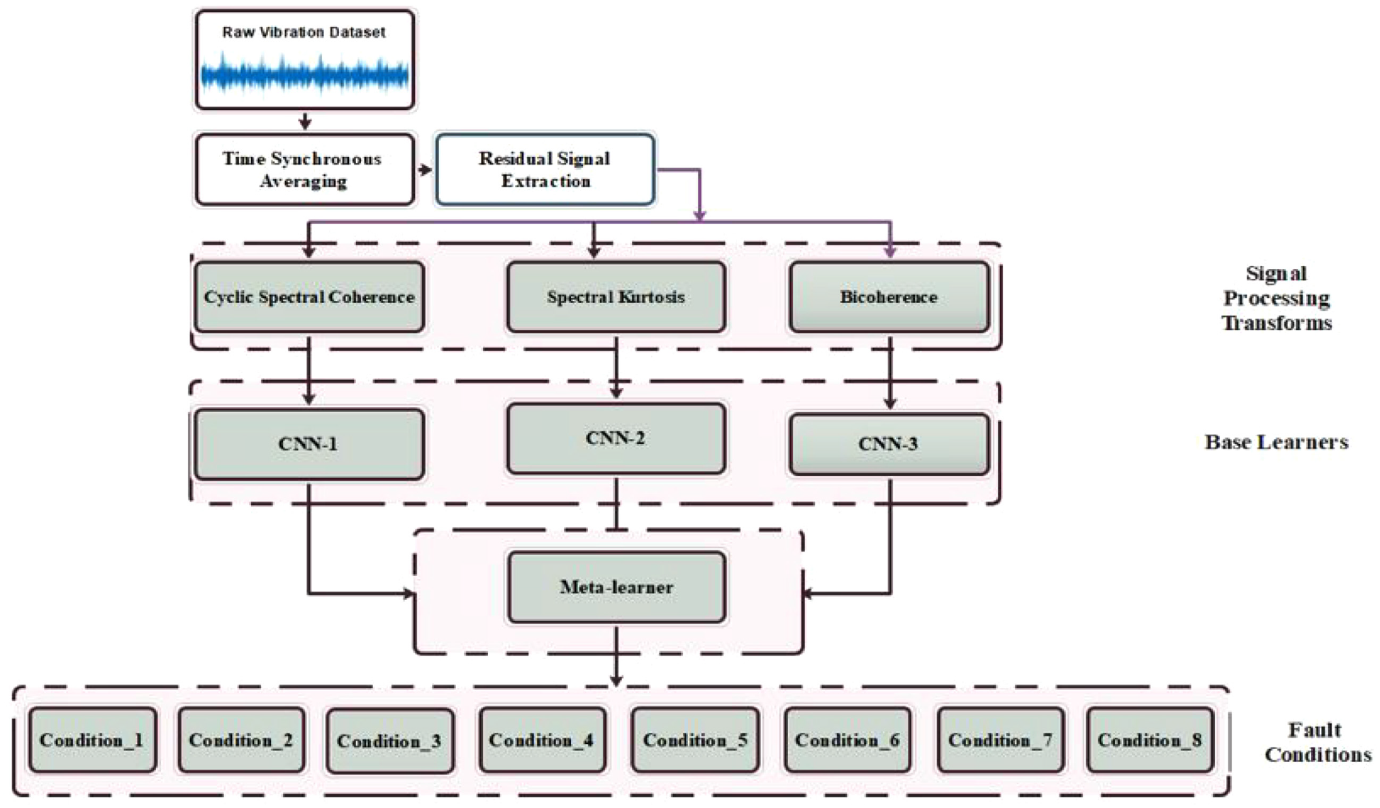
Proposed architecture for gear diagnosis.

One of the key preprocessing steps here is the TSA⁴⁶ to remove periodic wave-form from non-periodic waveforms in the vibration dataset. This is achieved by averaging the vibration signal over each revolution.⁴⁷ TSA can be implemented through an algorithmic proposition by Bechhoefer and Kingsley⁴⁶ Mathematically, the TSA can be estimated using equation (1)

TSA = \frac{1}{N} \sum_{i}^{N} x_{i}

(1)

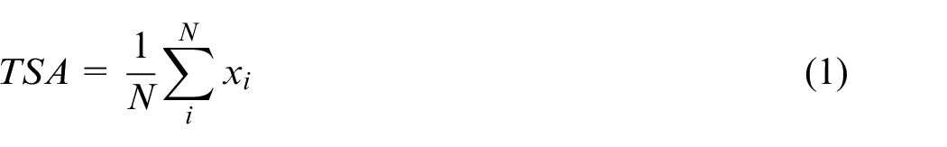
Where in equation (1), $x_{i}$ is the resampled vibration signal, N is the total number of segments of the signal, i is the index of the resampled signal segment. Residual signal is then obtained by removing the shaft frequency, gear mesh frequency and their harmonics.⁴ The learning techniques can be grouped into the base learners and the meta learner. The base learners are individual learners that learn directly from the preprocessed input dataset. The meta-learner on the other hand learns from the predictions of the base learners. Test is carried out with test dataset to ascertain the condition of the gear. Other elements of the proposed method include the various signal processing transform inputs on which the base learners are trained. As discussed in section 1 of this article, the selected signal processing transforms include cyclic spectral coherence, spectral kurtosis and bicoherence analysis.

Bicoherence

One of the Higher-Order Spectral Analysis methods is the bispectrum analysis, and its normalized version, the bicoherence analysis. They are an extension of the power spectrum. The bispectrum is related to the skewness of a signal and can be used to detect the asymmetric nonlinearities in a signal.⁴⁸ Bispectrum analysis provides a frequency domain measurement of the degree of coupling between three frequencies such as f₁, f₂ and f₁+f₂ components in a non-linearly interacting system.⁴⁹ The bispectrum estimation method can be obtained using the direct and indirect methods. However, the direct method is preferred because it is computationally less expensive.⁵⁰ Hence, the bispectrum of a signal can be estimated using equation (2):

B (f_{1}, f_{2}) = E [X (f_{1}) X (f_{2}) X^{*} (f_{1} + f_{2})]

(2)

Where E[.] is the expectation operation, * is the complex conjugate.

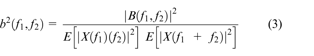
The variance of the bispectrum estimate is proportional to the triple product of the power spectrum. This results in a situation that can cause a misinterpretation of the results since the second-order properties of the vibration signal can dominate the bispectrum estimate.⁴⁸ Hence, this issue can be resolved by normalizing the bispectral estimate to obtain the bicoherence, as given by equation (3):

b^{2} (f_{1}, f_{2}) = \frac{{| B (f_{1}, f_{2}) |}^{2}}{E [| X (f_{1}) (f_{2}) |^{2}] E [| X (f_{1} + f_{2}) |^{2}]}

(3)

Cyclic spectral coherence

The vibration signal of a rotating machine operates in a way that will produce periodic signals under normal working conditions.⁹ A cyclostationary process is a stochastic process that exhibits hidden periodicity. There are different orders of cyclostationarity that can be defined based on the order of the moments. Hence an nth order cyclostationary signal is a signal whose nth-order statistic is periodic. These include first order, second order and third order.

The autocorrelation function of a second-order cyclostationary signal is periodic, and this conforms to equation (4):

R_{2 x} (t, τ) = R_{2 x} (t + T, τ) = E {x (t) x (t - τ)^{*}}

(4)

where $τ$ is the time lag, T is the period, E[.] is the expectation operation and $*$ is the complex conjugate.

The cyclic spectral correlation provides a tool for the description of the first order and second-order cyclostationary signals in the frequency-frequency domain,⁵¹ which can be expressed as equation (4).

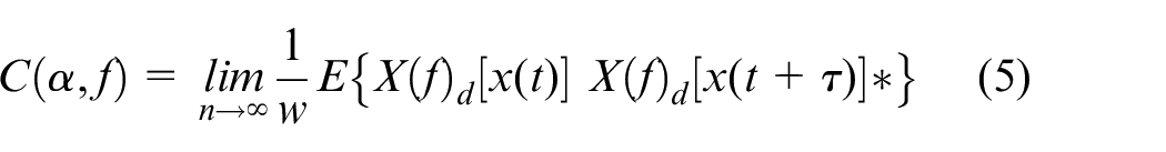
C (α, f) = \lim_{n \to \infty} \frac{1}{w} E {X {(f)}_{d} [x (t)] X {(f)}_{d} [x (t + τ)] *}

(5)

To minimize uneven distributions, a normalization of the Cyclic Spectral Correlation $C (α, f)$ gives a computation of the Cyclic Spectral Coherence ( $CSCoh$ ) in equation (6).

CSCoh (α, f) = \frac{C (α, f)}{{[C (0, f) C (0, f - α)]}^{\frac{1}{2}}}

(6)

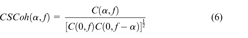
where $f$ is the spectral frequency which can be linked to the carrier component, and $α$ is the cyclic frequency related to modulation.

Spectral kurtosis

Antoni⁵² described spectral kurtosis based on the Wold-Cramer decomposition. It defines a non-stationary stochastic process as the output of a linear, causal, and time-varying system:

x (t) = \int_{- \infty}^{+ \infty} e^{j 2 π ft} H (t, f) d X (f)

(7)

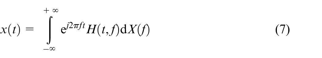
where H(t,f) is the time-varying function interpreted as the complex envelope of the process x(t) at a frequency “f,” and “dX(f)” is the unit variance of an orthogonal spectral process. The fourth-order normalized cumulant for a conditionally non-stationary process can be expressed by equation (8):

K_{x} (f) = \frac{〈 | H (t, f) |^{4} 〉}{{〈 | H (t, f) |^{2} 〉}^{2}} - 2

(8)

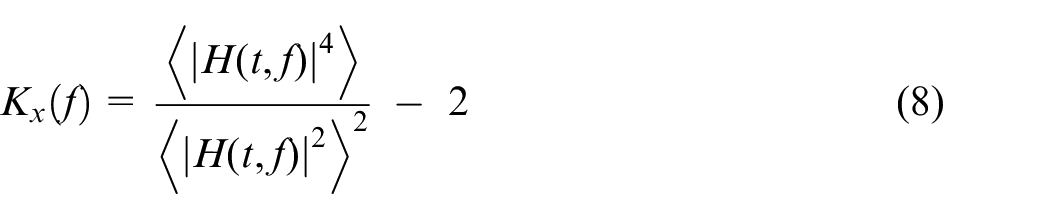
In equation (8), $H (t, f)$ is complex envelope at frequency $f$ , and $< \cdot >$ is the temporal average operator. However, when stationary additive noise is present, spectral kurtosis of the vibration signal can be computed through equation (9), where $ρ (f)$ is the noise to signal ratio at frequency f.

K_{x} (f) = \frac{K_{x} (f)}{{[1 + ρ (f)]}^{2}}

(9)

Convolutional neural network

CNN is a feed-forward model for processing grid-patterned data and is designed to automatically learn spatial hierarchies of features.⁵³ Generally, some layers of the CNN are the convolutional layer, pooling layer, and fully connected layer. The CNN has been useful in some diagnostic architecture for gear, bearing, and drive train faults.^54–56

The convolutional layer is important in CNN. It is made up of multiple learnable kernels or convolutional filters where the input image is convolved with the filters in that layer to give output feature maps.⁵⁷ The kernel is a grid of discrete numbers with each value known as the kernel weight. The results at the end of the convolution operation become input to the activation function to give the final output of the convolution layer.

Given an input to a CNN with size a × a × c, where a is the height and width of the image, and c represents the dept of the image or the channel. Let the convolutional filter be expressed as l × l × m where l is less than a, and m is less than or equal to the size of c. With the weight, $w^{'}$ , and bias terms, $b^{'}$ of the kernel, feature maps $h^{'}$ are generated. This is achieved at the convolutional layer by calculating the dot product between the weight of the kernel and the input data with the bias term added. The operation is expressed in equation (10) below:

h^{'} = ReLU (w^{'} * x + b^{'})

(10)

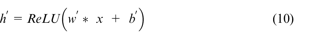
where ReLU is the activation function known as Rectified Linear Unit.

The pooling layer is the next layer of the CNN. This is where sub-sampling or down-sampling operation is carried out to shrink large size feature maps into smaller feature maps while upholding dominant features. Due to this operation, the network parameters are reduced and overfitting can be minimized.⁵⁷ Different types of pooling operation can be implemented such as maximum pooling layer, average pooling, and gated pooling.

The fully connected layer is found toward the end of the CNN model. Each of the neurons in this layer is connected to all neurons of the preceding layer.⁵⁷ High order abstractions obtained from features produced at other layers are used in this layer for decision making.

Ensemble model

The stack generalization approach was introduced by Wolpert.⁵⁸ It is an ensemble learning strategy in which many base models are trained, and combined through the use of a meta-learner to enhance the predictive strength of the models.⁴⁵ Stack generalization helps to reduce bias as well as the variance of the machine learning task. The meta-learner is trained based on input obtained by k-fold cross-validation. However, in cases where the value of k is large, a lot of resources are expended in the training process.⁴⁵

To overcome this challenge, a variation of stack generalization known as blending is used in this article. Amongst other advantages, blending ensemble is simple. A typical blending ensemble does not involve k-fold cross-validation. In blending, the predictions from different base models are used as training data for the meta-learner to approximate the target value.⁵⁹ In our proposed approach, the meta-learner is the multiclass Support Vector Machine (SVM). Regression and classification problems can be addressed with SVMs. The SVM works by making an optimal hyperplane to separate between the datasets, with the minimum distance between the data points described as support vector. Constrained quadratic optimization is used to achieve this objective by using structural risk minimization. Directed acyclic graphs, one versus one, and one versus all, are the techniques by which a multiclass SVM can be developed. One versus one coding design for eight classes is applied in this study through the Error-Correcting Output Code (ECOC) algorithm.⁶⁰

Experiment

Experimental setup

The Prognostic Health Management Society 2009 labeled gear dataset⁶¹ is used in this article. Figure 2(a) and (b) show the details of the experimental setup.

Figure 2.

(a) Experimental setup⁶¹ and (b) Plan view of the gearbox.⁶¹

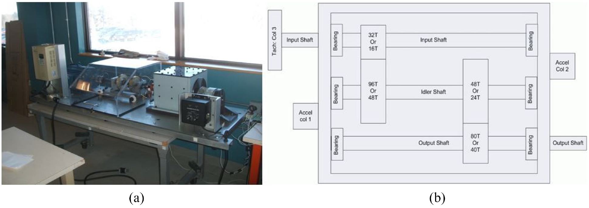
The experimental setup comprises four bearings, gears, input shaft, idler shaft, output shaft, and two accelerometers which are mounted on the input and output shaft retaining plates to measure the vibration signal. The two accelerometers are Endevco 6259M31 accelerometers having a sensitivity of 10 mV/g, with an error of ±1%, and mounted resonance frequency of >45 kHz. Additionally, an attached tachometer produces 10 pulses per revolution, thus providing accurate zero-crossing information. The gear types include spur gear and the helical gear. The dataset acquired for the spur gear was different from that collected for the helical gear conditions.

In this article, only the signal representing the spur gear is used. In Figure 2(b), T denotes the number of teeth. The number of teeth on the spur gear mounted on the input shaft is 32. The idle shaft has two spur gears mounted on it. Hence, the spur gear has 96 teeth which meshes with the spur gear having 32 teeth on the input shaft. Similarly, the spur gear having 48 teeth meshes with spur gear having 80 teeth, which is mounted on the output shaft. Since the gear faults information are mostly hidden in the high-frequency band,⁶² this dataset was collected at a sampling frequency of 66.67 kHz for 4 s.

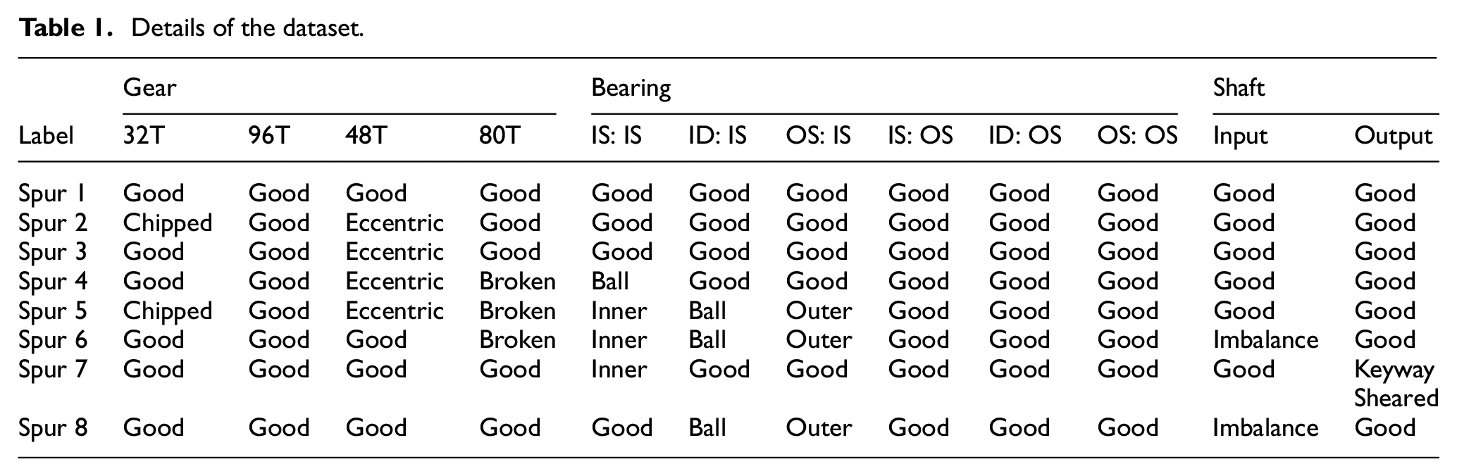
The spur gear dataset was collected at low and high load conditions at rotating speed conditions of 30, 35, 40, 45, and 50 Hz. Each of the data files is made up of three columns where column one is the input voltage, column two is the output voltage, and column three is the tachometer. There are eight labeled signals of the gearbox namely: spur 1, spur 2, spur 3, spur 4, spur 5, spur 6, spur 7, and spur 8. Some of the gear faults include chipped tooth, eccentric gear, and broken tooth. In Table 1, the spur 2 signal shows a case of multiple faults in the gear. Here, chipped tooth fault and eccentric gear fault are present in that signal. The gear chipped tooth and broken can be caused by initial fatigue damage, and progressing fatigue crack, respectively. The eccentric gear can be attributed to assembly and manufacturer errors. Also in Table 1, more details of the signal types and their labels are shown, IS:IS represents Input Shaft : Input Slide, ID:OS is the Idler Shaft : Output Slide and OS is the Output Shaft.

Table 1.

Details of the dataset.

	Gear				Bearing						Shaft
Label	32T	96T	48T	80T	IS: IS	ID: IS	OS: IS	IS: OS	ID: OS	OS: OS	Input	Output
Spur 1	Good	Good	Good	Good	Good	Good	Good	Good	Good	Good	Good	Good
Spur 2	Chipped	Good	Eccentric	Good	Good	Good	Good	Good	Good	Good	Good	Good
Spur 3	Good	Good	Eccentric	Good	Good	Good	Good	Good	Good	Good	Good	Good
Spur 4	Good	Good	Eccentric	Broken	Ball	Good	Good	Good	Good	Good	Good	Good
Spur 5	Chipped	Good	Eccentric	Broken	Inner	Ball	Outer	Good	Good	Good	Good	Good
Spur 6	Good	Good	Good	Broken	Inner	Ball	Outer	Good	Good	Good	Imbalance	Good
Spur 7	Good	Good	Good	Good	Inner	Good	Good	Good	Good	Good	Good	Keyway Sheared
Spur 8	Good	Good	Good	Good	Good	Ball	Outer	Good	Good	Good	Imbalance	Good

Application of the proposed method

Data preprocessing and data split

The data processing step starts with performing TSA on the entire dataset. The TSA and all other processing were performed using MATLAB^®. Residual signal extraction was performed on the result of the TSA operation to remove the shaft frequency, gear mesh frequency and their harmonics. Figure 3 shows the time domain plots of the residual signal for one rotation of the shaft. Three complimentary signal processing techniques were selected and used to obtain an extended feature set with spectral kurtosis, cyclic spectral coherence, and bicoherence analysis.

Figure 3.

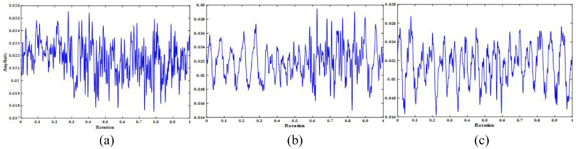
Residual signal of: (a) Spur 1, (b) Spur 2, and (c) Spur 3.

The spectral kurtosis plots or kurtogram were obtained using a maximum decomposition level for the chosen length of signal. The kurtogram is indicated in a combination of frequency (f, Δf) plane as shown in Figure 4. In this article, 400 kurtogram of size 224 × 224 × 3 pixels were created as inputs to the CNN-2 which constituted the 280 kurtogram for training, 60 kurtogram for validation, and 60 kurtogram for testing.

Figure 4.

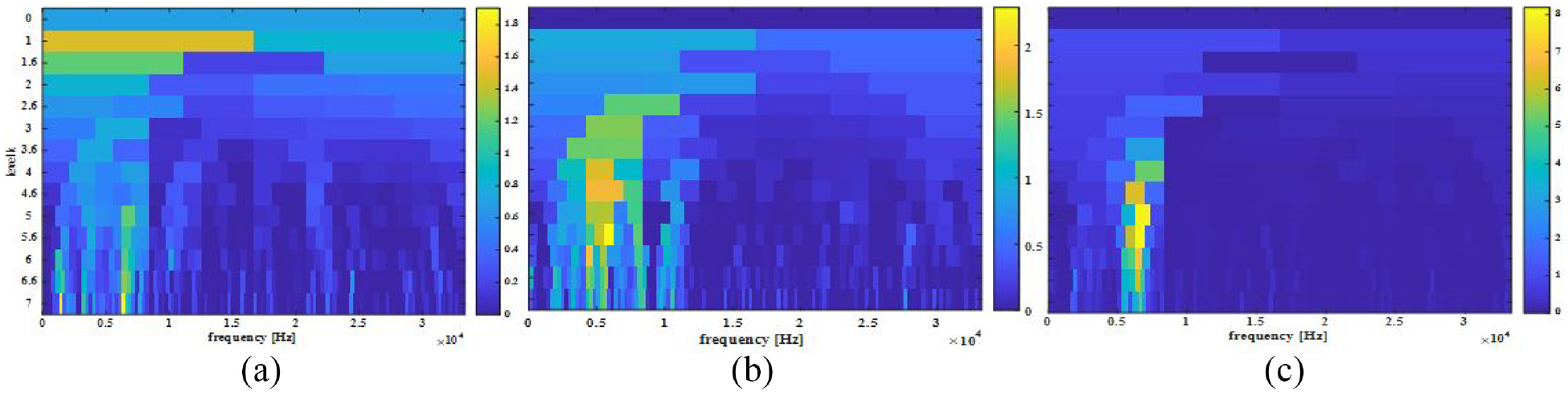
Kurtogram of: (a) Spur 1, (b) Spur 2, and (c) Spur 3.

One of the key considerations when generating the cyclic spectral coherence maps was the computational cost. Hence, a frame size that could allow for fast computations as well as obtaining good plots were used. Here, 12,925 data points were utilized in the creation of each of the cyclic spectral coherence maps. The window length chosen was 256, with the highest cyclic frequency to be scanned as 300 Hz. These parameters are different from the example shown in Figure 5. Figure 6 shows the Cyclic Spectral Coherence maps for spur 1, spur 2, and spur 3. Hence, cyclic spectral coherence components defined in terms of cyclic and linear frequency form the maps, which constitute inputs to CNN-1.

Figure 5.

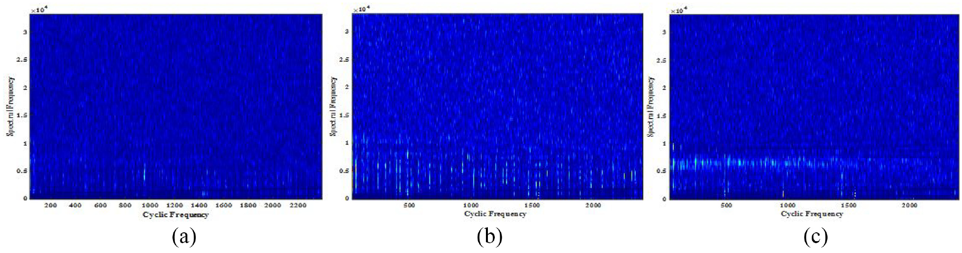
Cyclic spectral coherence map of: (a) Spur 1, (b) Spur 2, and (c) Spur 3.

Figure 6.

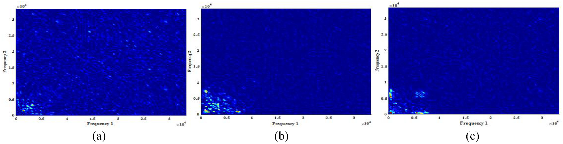
Bicoherence map of: (a) Spur 1, (b) Spur 2, and (c) Spur 3.

Similar to the kurtogram, and cyclic spectral coherence maps, the bicoherence maps were composed of a training set of 280 images for each signal transform. Figure 6 represents bicoherence maps which indicate interactions between spectral components at frequencies component f1 and f2. These maps form inputs to the CNN-3. The validation set for each transform was made of 60 images, and the testing set for each transform was made of 60 images. In Table 2, the detailed specifications of the training, validation, and testing datasets for each of the machine signals described in Table 1 are provided.

Table 2.

Details of the training, validation, and testing vibration dataset.

Set	Images	Runs	S, LL & HL
Training	280	1 & 2	30–40 (LL–HL)
Validation	60	1 & 2	45 LL–50 HL
Testing	60	1 & 2	50 HL–50 LL

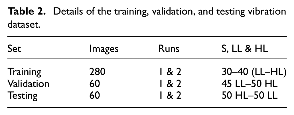
Where in Table 2, S, LL, and HL represent the speed, low load, and high load conditions of the machine, “run one” refers to data collected during the first operation of the test rig, “run two” represents the dataset collected at the second operation of the machine.

Learners

The base learners are the individual learners on which the preprocessed datasets are trained. They are presented with images processed using the selected signal processing transforms. Hence, creating the cyclic spectral coherence model branch, spectral kurtosis model branch, and bicoherence model branch of the ensemble. Parameters such as the initial learning rate were set at 0.001 for each of the branches. Table 3 shows the structure of CNN-1, CNN-2, and CNN-3; with CNN-1 being the “convolutional neural network one,” CNN-2 the “convolutional neural network two,” and CNN-3 is the “convolutional neural network three.”

Table 3.

Structure of the base learners.

Name	CNN-1	CNN-2	CNN-3
Input	224 × 224 × 3	224 × 224 × 3	224 × 224 × 3
Conv_1	8 × 3 × 3 × 3	8 × 5 × 5 × 3	8 × 3 × 3 × 3
Maxpool_1	3 × 3	3 × 3	3 × 3
Conv_2	16 × 3 × 3 × 8	16 × 5 × 5 × 8	8 × 3 × 3 × 8
Maxpool_2	3 × 3	3 × 3	3 × 3
Conv_3	32 × 3 × 3 × 16	32 × 5 × 5 × 16	16 × 3 × 3 × 8
Maxpool_3	3 × 3	3 × 3	3 × 3
Conv_4	64 × 3 × 3 × 32	64 × 5 × 5 × 32	32 × 3 × 3 × 16
dropout	40	75	70
Fully Connected	Fully Connected	Fully Connected	Fully Connected
SoftMax	1	1	1
Output	8	8	8

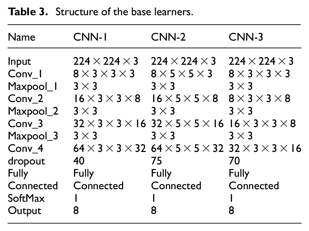
Some data augmentation techniques were implemented to improve the attribute of the data and also increase the data size.⁵⁷ These included safe image rotation between – 20° and 20°. With the training dataset being in the central position, vertical and horizontal translation were implemented on them. This involve images in the training set being moved down, up, left, or right to overcome position bias. The vertical and horizontal translations were set to −5 to 5 pixels. The training duration of the model based on proposed method was 13,680 s. This was carried out using Intel(R) Core(TM) i7-8550U single CPU at 1.8 GHz and useable RAM size of 7.87 GB.

Performance evaluation

To ascertain the performance of the proposed architecture, different metrics were used. These include F1-Score, accuracy, recall, precision, false-positive rate, false-negative rate, Receiver operating characteristic curve and Area Under the Curve. Mathematically, these metrics are expressed in equations (11)–(16).

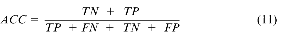
(1) The accuracy is the ratio of the number of correct predictions to the total number of predictions. However, accuracy alone as a performance metric is not to be relied on. This is because when working with an imbalanced dataset, even a model with zero predictability could still give high accuracy. Accuracy is given by equation (11); where ACC is accuracy, TN is true negative, TP is true positive, FN is false negative, and FP is false positive.

ACC = \frac{TN + TP}{TP + FN + TN + FP}

(11)

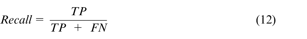
(2) The recall is a metric that states the portion of the actual positive samples that were correctly identified. It shows the samples belonging to a class that were correctly classified. It is given by equation (12):

Recall = \frac{TP}{TP + FN}

(12)

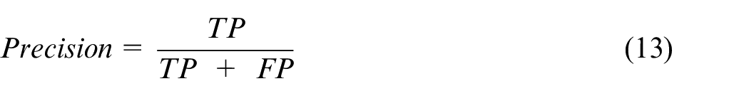
(3) Precision is a performance metric that defines the ratio of correctly classified positive samples to the number of samples that the network labels as positive. It is given as equation (13):

Precision = \frac{TP}{TP + FP}

(13)

(4) The false-positive rate is also known as the false alarm rate. It gives the percentage of samples predicted to belong to each class that are incorrectly classified. This metric is very important because the cost of shutting down the machine when the machine is not faulty can be very high. It is expressed as FPR in equation (14):

FPR = \frac{FP}{TN + FP}

(14)

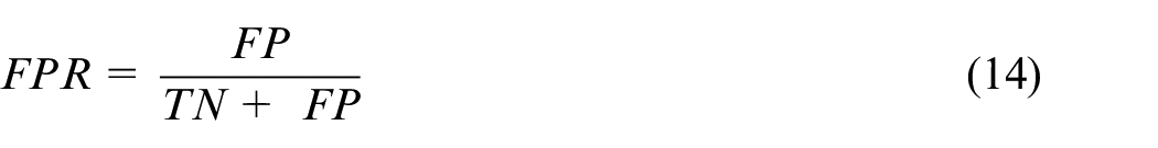
(5) The false-negative rate is the percentage that all the samples belonging to each class are incorrectly classified. Equation (15) gives the False Negative Rate (FNR) as:

FNR = \frac{FN}{TP + FP}

(15)

(6) The Receiver Operating Characteristic Curve (ROC) is a metric which shows the performance of each of the classification models at all the classification thresholds. It demonstrates how effectively a certain detector can separate groups in a quantitative way.⁶³ The ROC graph plots the True Positive Rates against the False Positive Rates.

(7) A closely related metric to the ROC graph is the Area Under the Curve (AUC). AUC indicates the ability of a classifier to avoid false classification. It measures the whole two-dimensional area underneath the ROC curve. The estimate of the ROC curve and the AUC are presented for the proposed method given in this article.

(8) The F1 score is the harmonic mean between the precision and the recall.

F 1 Score = 2 x \frac{Precision x Recall}{Precision + Recall}

(16)

Results and discussions

The proposed method for gear multiple fault diagnosis was developed from the use of extended feature sets on gear residual signal. Different metrics have been defined for the evaluation of the performance of the proposed methodology. Figures 7(a), (b) and 8 show the confusion matrixes of different CNN models using cyclic spectral coherence inputs, spectral kurtosis maps, and bicoherence maps respectively.

Figure 7.

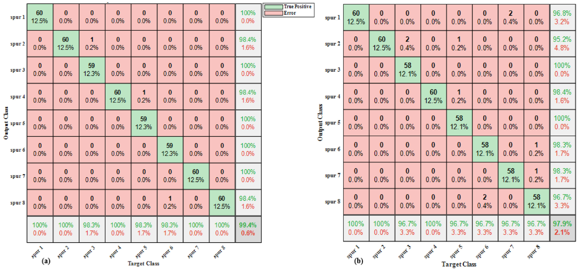
Confusion matrix of: (a) CNN-1 and (b) CNN-2.

Figure 8.

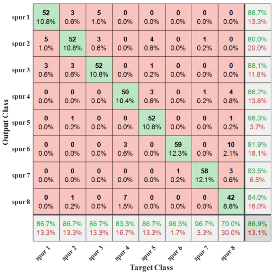
Confusion matrix for CNN-3.

Taking Figure 7(a) (CNN-1), the column shows the true class or output class, while the predicted class or target class is represented by the rows. The diagonal cells show the percentage and the number of correctly classified gear conditions by the trained model. The second cell on the diagonal shows that 60 observations represent 12.5% of the 480 total test datasets used in testing. These were classified as having chipped tooth and eccentric faults in the spur 2 signal. The test accuracies of these models on the test dataset are shown on the last cell on the far right of the confusion matrixes.

The validation accuracy of the CNN-1, CNN-2, and CNN-3 models trained independently, was found to be 98.54%, 94.58%, and 88.95%, respectively. While the test accuracy of these models was 97.71% for CNN-1, 93.80% for CNN-2, and 86.90% for CNN-3. In the CNN-1 model, the overall precision was 0.9775 and a recall of 0.9771. The CNN-2 model produced a precision of 0.9390 and a recall of 0.9375, while the last model, CNN-3 outputs a precision of 0.8710 and an overall recall of 0.8688.

Considering the signals with case label spur 1, spur 2 where multiple faults is present, and spur 3 where a single fault is present, the confusion matrix in Figure 7(a) is used as a representative case for analysis of the single and multiple faults misclassification. For the rows of this confusion matrix, the predicted class, out of 62 spur 1 predictions, a precision of 96.8% was obtained, and 3.2% constituted the false positive rate. Similarly, out of the 63 spur 2 predictions, 60 of them were true positives, while 3 were false positives – belonging to signals with case label spur 3 and spur 5. Considering spur 3 on the confusion matrix, there was a positive predictive value of 100% and a false positive of 0%.

In the column of the confusion matrix, out of the combined 120 spur 1 and spur 2 cases, CNN-1 indicated a recall of 100%, while recording a 0% false negative rate for the respective classes. Of the 60 spur 3 cases, 96.7% were correctly predicted to be spur 3 and 3.3% were predicted to be spur 2. Hence, the reason for this misclassification between signal with case label spur 3 and spur 2 can be attributed to spur 2 being a multiple faulted signal consisting of a fault type present in the signal case (spur 3) from the same gear. That is, the signal spur 2 is made up of chipped tooth gear fault and eccentric gear fault, while the signal with label spur 3 is made up of eccentric gear fault which has the same physical principle as that of a constituent of spur 2.

Among the single models, the CNN-3 model had the lowest overall effectiveness. A reason for this is the presence of spurious peaks which may not be related to the fault may appear as quadratic phase coupling. Also, the choice of the number of samples to constitute a segment can limit the accuracy. CNN-1 showed the best performance amongst the single models. This is because the cyclic spectral coherence provides a comparative advantage in analyzing signatures with non-linearity, non-stationarity and non-gaussianity.⁹

Figure 9(a) shows the confusion matrix of the proposed method using multiclass SVM as meta learner. Based on the proposed approach, the performance of the trained model was also evaluated using the same performance metrics as those of the individual models. The overall test accuracy of the proposed model BECNN-SVM was 99.40%, the overall precision and the overall recall were 0.9939 and 0.9938 respectively. However, to examine the performance of the proposed model using a meta learner that operates on another algorithm, the decision tree was used as an alternative meta learner to obtain the so-called BECNN-DT. Figure 9(b) represents a confusion matrix that has a decision tree as the meta learner. This alternative model had an overall test accuracy of 97.90%, the overall precision was 0.9792, and the overall recall was 0.9798.

Figure 9.

Proposed model’s confusion matrix: (a) BECNN-SVM and (b) BECNN-DT.

Taking signals with case label spur 1, spur 2 and spur 3 in the confusion matrix of the proposed model BECNN-SVM in Figure 9(a). It indicates that for spur 1, there was 0% false positive rate and false negative rate. That is, while the gear was predicted by the model to be spur 2, it was actually of that case label. Although, there was 1.6% false positive rate and 0% false negative rate for spur 2, the proposed model predicted 0% false positive rate and 1.7% false negative rate for spur 3. It can be observed that among the models’ confusion matrixes, the proposed ensemble model BECNN-SVM, returned the lowest misclassification rates.

As one of the common methods to estimate the detection performance of the models, the ROC curves for CNN-1, CNN-2, CNN-3, BECNN-DT, and the proposed model, are shown in Figures 10 and 11 of this article. During the comparison of the ROC curves of different tests, the worst curve lies closer to the diagonal while the best curve lies closer to the top left corner of the curve.⁶³ Hence, taking the ROC curves in Figure 10(a) to (c), it was observed that while CNN-1’s ROC curve lies closest to the top left corner, spur 1 in the same figure showed the best performance with AUC of 1. On the other hand, the presented single models achieved the best performance for mean AUC of 0.9975 with spur 7 and worst performance with spur 8 having a mean AUC of 0.9804.

Figure 10.

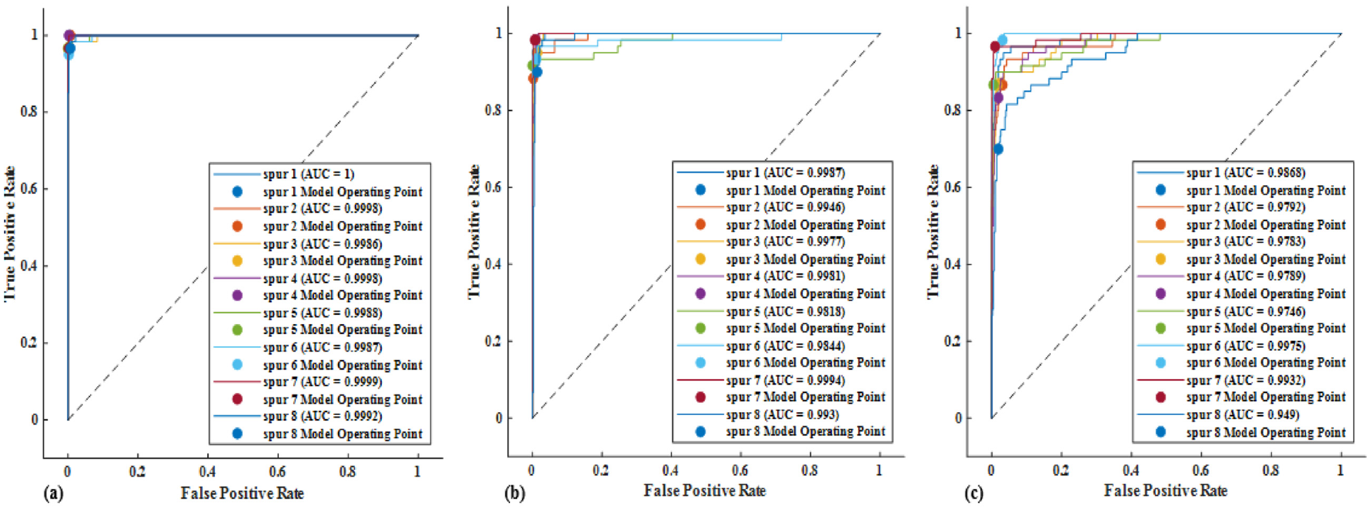
Receiver characteristic curve of: (a) CNN-1, (b) CNN-2 and (c) CNN-3.

Figure 11.

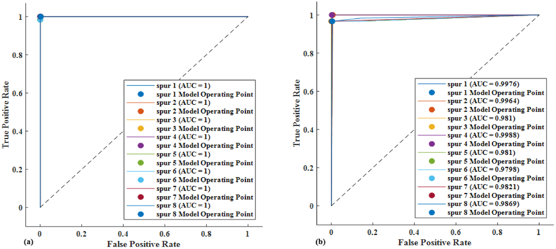
Receiver characteristic curve of: (a) The proposed model BECNN-SVM and(b) BECNN-DT.

Figure 11(a) shows the ROC curve for the proposed model (BECNN-SVM). It has the overall best performance across all classes and models with an AUC of 1. Figure 11(b), a comparative model, indicates a ROC curve that is not as good as that of the BECNN-SVM with an AUC less than 1 amongst the classes.

A variety of deep ensemble learning has been proposed for gear diagnosis in literature. The overall accuracy of these methods is shown in Table 4 for comparison with our results.

Table 4.

Performance comparison with existing techniques.

Reference	Method	Part	ACC (%)	Precision (%)	Recall (%)	F1 Score
Hsiao et al.³⁷	Ensemble CNN + FCN	Gearbox	97.30	0.9710	0.9730	0.9720
Yu³⁸	SSDAE-NCL	Gearbox	98.80	N/A	N/A	N/A
Han et al.³⁹	Dynamic CNN	Gearbox	96.48 (Case 1)	N/A	N/A	N/A
Han et al.³⁹	Dynamic CNN	Gearbox	91.30 (Case 2)	N/A	N/A	N/A
Senanayaka et al.⁴¹	MLP + CNN	Gearbox (mixed faults) fault	96.07 (mean)	N/A	N/A	N/A
Zhang et al.⁴²	EDCAE (Ensemble)	Gearbox and Bearings	96.6 (mean)	N/A	N/A	N/A
Pang et al.⁴³	Ensemble kernel extreme	Gearbox	95.20	0.9520	0.9519	0.9519
Proposed	BECNN-SVM	Gearbox	99.40	0.9939	0.9938	0.9938

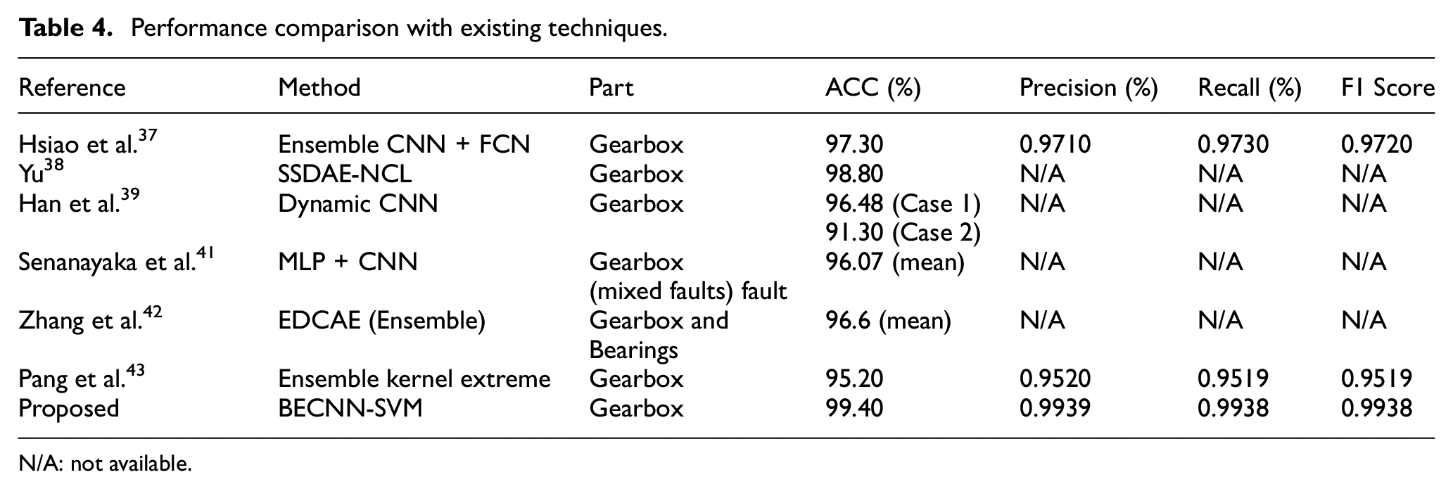
N/A: not available.

The average accuracy of all the models in Table 4 was 95.96% compared to 99.40% obtained using the proposed approach. This implies that on the average, our method outperformed these approaches by 3.44%.

Conclusion

An approach for multiple fault diagnosis of gears was implemented in this research. Three signal processing techniques were utilized in preprocessing gear residual signals for intelligent diagnosis of gear faults. Being simpler and straightforward, the deep blending ensemble learning method was developed for gear diagnosis. BECNN-SVM showed increased overall effectiveness when compared with the best individual models and state-of-the-art methods. The complementary nature of the transforms entailed that the approach is flexible to new faults scenario input to the system. For instance, while the training was based on 30–40 Hz speed and low-high load conditions, testing of the models’ overall effectiveness was based on 50 Hz speed and low-high load conditions.

Footnotes

Declaration of conflicting interests

The author(s) declared no potential conflicts of interest with respect to the research, authorship, and/or publication of this article.

Funding

The author(s) disclosed receipt of the following financial support for the research, authorship, and/or publication of this article: This work was funded by Petroleum Technology Development Fund (PTDF) and the Integrated Vehicle Health Management Centre, Cranfield University.

ORCID iD

Udeme Ibanga Inyang

References

Jiang

, et al. Recent progress on decoupling diagnosis of hybrid failures in gear transmission systems using vibration sensor signal: a review. Meas J Int Meas Confed 2016; 90: 4–19.

Statoil. Investigation into helicopter safety in Statoil following the Turøy helicopter. 2016; 1–70.

Aherwar

. An investigation on gearbox fault detection using vibration analysis techniques: A review. Aust J Mech Eng 2012; 10: 169–183.

Jablonski

. Springer tracts in mechanical engineering. Condition monitoring algorithms in MATLAB^®. Cham: Springer, 2020.

KiranKumar

Lokesha

Kumar

, et al. Review on condition monitoring of bearings using vibration analysis techniques. IOP Conf Ser Mater Sci Eng 2018; 376 012110.

Večeř

Kreidl

Šmíd

. Condition Indicators for gearbox condition monitoring systems. Acta Polytechnica 2005; 45: 35–43.

Zhou

Wang

, et al. Online condition diagnosis for a two-stage gearbox machinery of an aerospace utilization system using an ensemble multi-fault features indexing approach. Chin J Aeronaut 2019; 32: 1100–1110.

Vanraj Dhami

Pabla

. Gear fault classification using vibration and acoustic sensor fusion: a Case Study. In: Proceedings of the 2018 condition monitoring and diagnosis, Perth, Australia, 23–26 September 2018, pp.1–6. Piscataway, NJ: IEEE.

Tang

Yuan

Zhu

. Cyclostationary analysis towards fault diagnosis of rotating machinery. Processes 2020; 8: 1217–1315.

10.

Kundu

Darpe

Kulkarni

. A review on diagnostic and prognostic approaches for gears. Struct Health Monit. Epub ahead of print 23 December 2020. DOI: 10.1177/1475921720972926

11.

Feng

Chu

. Cyclostationary analysis for gearbox and bearing fault diagnosis. Shock Vib 2015; 2015: 1–12.

12.

Afia

Rahmoune

Benazzouz

. Gear fault diagnosis using autogram analysis. Adv Mech Eng 2018; 10: 1–11.

13.

Gelman

Petrunin

Jennions

, et al. Diagnostics of local tooth damage in gears by the wavelet technology. Int J Progn Heal Manag 2020; 3: 1–7.

14.

Wang

. Research on fault diagnosis of gearbox with improved variational mode decomposition. Sensors 2018; 18: 3510.

15.

Wang

Cheng

. A method for the compound fault diagnosis of gearboxes based on morphological component analysis. Meas J Int Meas Confed 2016; 91: 519–531.

16.

Zhang

, et al. Gearbox composite fault diagnosis method based on minimum entropy deconvolution and improved dual-tree complex wavelet transform. Entropy 2018; 21: 1–23.

17.

Praveenkumar

Saimurugan

Ramachandran

. Intelligent fault diagnosis of synchromesh gearbox using fusion of vibration and acoustic emission signals for performance enhancement. Int J Progn Heal Manag 2019; 10: 1–11.

18.

Rafiee

Arvani

Harifi

, et al. Intelligent condition monitoring of a gearbox using artificial neural network. Mech Syst Signal Process 2007; 21: 1746–1754.

19.

Wang

. K-nearest neighbors based methods for identification of different gear crack levels under different motor speeds and loads: Revisited. Mech Syst Signal Process 2016; 70-71: 201–208.

20.

Jiang

Wang

, et al. Multi-mode separation and nonlinear feature extraction of hybrid gear failures in coal cutters using adaptive nonstationary vibration analysis. Nonlinear Dyn 2016; 84: 295–310.

21.

Chen

Sánchez

. Multi-layer neural network with deep belief network for gearbox fault diagnosis. J Vibroengineering 2015; 17: 2379–2392.

22.

Han

Yang

Ren

, et al. Comparisons of different deep learning-based methods on fault diagnosis for geared system. Int J Distrib Sens Netw 2019; 15: 1–17.

23.

Chen

Liu

Tang

, et al. A novel fusion approach of deep convolution neural network with auto-encoder and its application in planetary gearbox fault diagnosis. Proc IMechE, Part O: J Risk and Reliability 2021; 235: 3–16.

24.

Zhang

, et al. Gear pitting fault diagnosis using disentangled features from unsupervised deep learning. Proc IMechE, Part O: J Risk and Reliability 2018; 233: 719–730.

25.

Rexnord Industries. Failure analysis. Gears-Shafts-Bearings-Seals. 1978; 2: 1–20.

26.

Hassan

Coats

Shin

, et al. Bicoherence analysis for condition assessment of multi-faulted helicopter drivetrain systems. Ann Forum Proc. 2012; 4: 2326–2331.

27.

Gelman

Solinski

Shaw

, et al. Vibration diagnosis of a gearbox by wavelet bicoherence technology. Insight Non-Destr Test Cond Monit 2017; 59: 440–444.

28.

Fackrell

JWA

McLaughlin

White

. Practical issues concerning the use of bicoherence for the detection of quadratic phase coupling. In: Proceedings of the 4th IEEE workshop on higher order statistics, Spain.

29.

Kim

Powers

Grady

, et al. A novel QPC detector for the health monitoring of rotating machines. In: 2007 IEEE instrumentation & measurement technology conference IMTC, 2007, pp.1–6.

30.

Wang

Xiang

Markert

, et al. Spectral kurtosis for fault detection, diagnosis and prognostics of rotating machines: a review with applications. Mech Syst Signal Process 2016; 66–67: 679–698.

31.

Gelman

Kolbe

Shaw

, et al. Novel adaptation of the spectral kurtosis for vibration diagnosis of gearboxes in non-stationary conditions. Insight Non-Destr Test Cond Monit 2017; 59: 434–439.

32.

Combet

Gelman

. Optimal filtering of gear signals for early damage detection based on the spectral kurtosis. Mech Syst Signal Process 2009; 23: 652–668.

33.

Mauricio

Gryllias

. Vibration-based condition monitoring of wind turbine gearboxes based on cyclostationary analysis. J Eng Gas Turbine Power 2019; 141: 1–8.

34.

Mauricio

Smith

, et al. Vibration based condition monitoring of planetary gearboxes operating under speed varying operating conditions based on cyclo-non-stationary analysis. Springer Nature Switzerland AG 2019. DOI: 10.1007/978-3-319-99268-6_19.

35.

Minghang

Kang

Tang

, et al. An Ensemble Learning-based fault diagnosis method for rotating machinery. IEEE Trans Ind Electron 2018; 63: 245–255.

36.

Cao

Geddes

Yang

JYH

, et al. Ensemble deep learning in bioinformatics. Nat. Mach. Intell 2020; 2: 500–508.

37.

Hsiao

Shivam

Kam

. Fault diagnosis method for worm gearbox using convolutional network and ensemble learning. J Phys Conf Ser 2020; 1509; 012030.

38.

. A selective deep stacked denoising autoencoders ensemble with negative correlation learning for gearbox fault diagnosis. Comput Ind 2019; 108: 62–72.

39.

Han

Tang

Deng

. Multi-level wavelet packet fusion in dynamic ensemble convolutional neural network for fault diagnosis. Meas J Int Meas Confed 2018; 127: 246–255.

40.

Zhang

, et al. Fault diagnosis of rotating machinery based on improved wavelet package transform and SVMs ensemble. Mech Syst Signal Process 2007; 21: 688–705.

41.

Senanayaka

JSL

Van Khang

Robbersmyr

. Multiple classifiers and data fusion for robust diagnosis of gearbox mixed faults. IEEE Trans Industr Inform 2019; 15: 4569–4579.

42.

Zhang

Gao

, et al. Ensemble deep contractive auto-encoders for intelligent fault diagnosis of machines under noisy environment. Knowl. Based Syst 2020; 196: 105764.

43.

Pang

Yang

Zhang

, et al. Fault diagnosis of rotating machinery with ensemble kernel extreme learning machine based on fused multi-domain features. ISA Trans 2020; 98: 320–337.

44.

Nguyen

Bao

Tew

, et al. Ensemble based real-time adaptive classification system for intelligent sensing machine diagnostics. IEEE Trans Reliab 2012; 61: 303–313.

45.

Chatzimparmpas

Martins

Kucher

, et al. Empirical study: visual analytics for comparing stacking to blending ensemble learning. In: Proceedings of 2021 23rd international conference on control systems and computer science (CSCS), 2021, pp.1–8.

46.

Bechhoefer

Kingsley

. A review of time synchronous average algorithms. In: Annual conference of the PHM Society, 2009, pp.1–10.

47.

Sim

Kim

Park

, et al. A tutorial for feature engineering in the prognostics and health management of gears and bearings. Appl Sci 2020; 10: 5639.

48.

Rivola

. Applications of higher order spectra to the machine condition monitoring, Bologna, luglio 2000 Viale Risorgimento, 2-4 40136 Bologna. DIEM, 2000, pp.2–4.

49.

Yang

Stronach

MacConnell

. The application of advanced signal processing techniques to induction motor bearing condition diagnosis. Meccanica 2003; 38: 297–308.

50.

Saidi

Ali

Fnaiech

. Bi-spectrum based-EMD applied to the non-stationary vibration signals for bearing faults diagnosis. ISA Trans 2014; 53: 1650–1660.

51.

Liu

Gryllias

. A semi-supervised support vector data description-based fault detection method for rolling element bearings based on cyclic spectral analysis. Mech Syst Signal Process 2020; 140: 106682.

52.

Antoni

. The spectral kurtosis: a useful tool for characterising non-stationary signals. Mech Syst Signal Process 2006; 20: 282–307.

53.

Yamashita

Nishio

RKG

, et al. Convolutional neural networks: an overview and application in radiology. Insights Imaging 2018; 9: 611–629.

54.

Zhao

Yan

Chen

, et al. Deep learning and its applications to machine health monitoring. Mech Syst Signal Process 2019; 115: 213–237.

55.

Liu

Cai

, et al. Lightweight deep residual CNN for fault diagnosis of rotating machinery based on depthwise separable convolutions. IEEE Access 2019; 7: 57023–57036.

56.

Benkedjouh

Zerhouni

Rechak

. Deep learning for fault diagnosis based on short-time Fourier transform. In: 2018 International conference on Smart Communications in Network Technologies (SaCoNeT), 2018, pp.288–293.

57.

Alzubaidi

Zhang

Humaidi

, et al. Review of deep learning: concepts, CNN architectures, challenges, applications, future directions. J Big Data. 2021; 8(1):53.

58.

Wolpert

. Stacked generalization. Neural Netw 1992; 5: 241–259.

59.

Chen

Tanaka

Kotera

, et al. Comparison and improvement of the predictability and interpretability with ensemble learning models in QSPR applications. J Cheminform 2020; 12: 19.

60.

Mathworks. Statistics and machine learning toolbox user’s guide, 2021, p.202. https://uk.mathworks.com/help/stats/classificationecoc.html (accessed January 3, 2022)

61.

PHM Society. PHM Society data challenge2009, https://www.phmsociety.org/competition/PHM/09 (accessed July 16, 2021).

62.

Lei

Yang

Jiang

, et al. Applications of machine learning to machine fault diagnosis: a review and roadmap. Mech Syst Signal Process 2020; 138: 106587.

63.

Saidi

Fnaiech

Henao

, et al. Diagnosis of broken-bars fault in induction machines using higher order spectral analysis. ISA Trans 2013; 52: 140–148.

A composite learning approach for multiple fault diagnosis in gears

Abstract

Keywords

Introduction

Materials and methods

Bicoherence

Cyclic spectral coherence

Spectral kurtosis

Convolutional neural network

Ensemble model

Experiment

Experimental setup

Application of the proposed method

Data preprocessing and data split

Learners

Performance evaluation

Results and discussions

Conclusion

Footnotes

Declaration of conflicting interests

Funding

ORCID iD

References