
Abstract
Considerable benefits have been gained from condition-based maintenance (CBM) utilizing continuous monitoring integrated with information technology. However, periodic inspection for CBM is still used widely as a practically helpful method to know the condition of the equipment. This paper starts from a case study where a maintenance log recorded by periodic inspection from five hydrant pumps is used to estimate the required parameter for maintenance modeling. To process the data for CBM, two schemes are taken into consideration: Inference of condition indicator through repair activities and reflection of non-observable events with virtual nodes. A CBM model of inspection-based preventive maintenance with discrete data is developed using the Markov model. The semi-Markov process is adopted then with more flexibility allowing the Weibull distributed sojourn times and the Multiphase Markov process is suggested to reflect the periodic inspection. Thus, the model for pumps takes into account both SMP and multiphase Markov process. Monte-Carlo simulations are generated to calculate state probability and the number of maintenances. An analytical solution is proposed by the transition probability of embedded Markov chain (EMC) and sojourn time of SMP. The developed CBM models are verified and compared based on analysis results and empirical data.
Introduction
With the development of sensing and information technology, condition-based maintenance (CBM) has been an effective approach for realizing cost-effective maintenance by combining reliability/maintenance models with sensor data collected by monitoring systems.1–3 However, in practices, real-time diagnosis is expensive to be adopted because it requires a bunch of equipment and a significant effort to train staff, 4 and inspections with some time intervals are more reasonable. In inspections, states of items are assessed by the condition indicators, degradation, and defects can be revealed and preventive actions can be then conducted before actual failures.
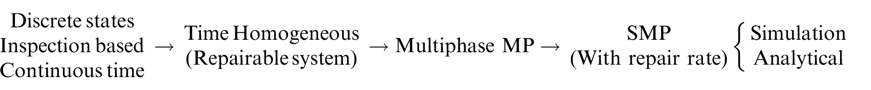
Although degradation of a physical system is continuous, it can be modeled in a discrete way with multiple health states for making decisions related to maintenance. A basic Markov process (MP) called time-continuous Markov chain (TCMC) is a commonly used tool to illustrate the degradation process in CBM, 1 provided that both continuous monitoring of the item and exponentially distributed sojourn times in each state are assumed. Such an assumption sometimes reveals Markov process’s restriction in the maintenance modeling. Firstly, contrary to the continuous monitoring system, when the item’s state is known at specific inspection dates and repair can be triggered only at these dates, the item has a special jump with a different transition rate matrix. Therefore, Markov process can not apply to the empirical data given by periodic inspections in this study, but multi-phase Markov process can be considered to allow the different transition rate matrixes of model changes by linking two phases. Secondly, the exponentially distributed sojourn times are too restrictive and might not fit the actual data. Considering more general sojourn times leads to Semi-Markov Process (SMP) suitable for analytical treatment. Thus, SMP does not possess a memoryless property, which contributes to being superior to Markov process in modeling the actual deterioration patterns of the system.
It is difficult to treat SMP models analytically. 5 Some attempts have been conducted to convert SMP models to MP models by approximating non-exponential distribution to exponential distribution for ease of solution. 6 With regard to an analytical approach for steady-state solution of SMP, the mean time spent in each state and the invariant distribution of the embedded Markov chain (EMC) are required. and consequently two stages made up of EMC and mean sojourn times have been suggested.6–8 In more cases, Monte Carlo simulation is introduced to determine the state probabilities and the amount of maintenance.
However, not so many existing studies on CBMs start from the empirical data, which needs pre-processing and acts as constraints on some modeling assumptions. From another perspective, researches on data processing can be well found, but few of them are directly related to CBMs or inspections. Thus, the objective of this paper is to develop and present the inspection-based maintenance modeling and analysis process starting from empirical case studies of collecting and processing empirical data.
The remainder of this paper is organized as follows: Section 2 describes the system in the case study where we collect data, and then Section 3 provides modeling approaches for the system. Empirical data is analyzed for estimating model parameters in Section 4. Then numerical studies are conducted with discussions in Section 5. Finally, Section 6 summarizes the results.
System description and qualitative analysis
Empirical data of this study is from hydrant pumps at fueling facilities in an airport, which are designed to pressurize fuel to convey into the hydrant pits placed near an aircraft through the underground pipes so that fuel is directly fed to the aircraft. A homogeneous sample of five hydrant pumps has been extracted for this study.
Normal inspections for such equipment are carried out on monthly basis besides daily patrol inspection, and replacement schedules comply with the maintenance manuals of the manufacturer. According to the maintenance log and manuals, a half-year inspection is a time to take a closer look at the pump in more details. To minimize the maintenance investment, repairs are done minimally by the level of keeping the basic demands. Unfortunately, no record of measurement indicating the condition of a pump, such as vibration level, is available due to being treated as volatile information not stored.
Degradation and maintenance
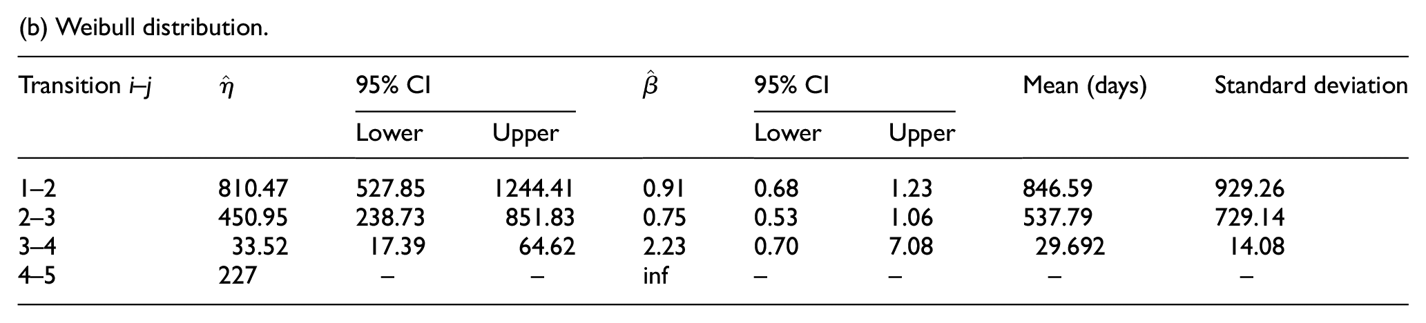
Maintenance activities are correlated with degradation. Basic assumptions include that the item with a long interval of maintenance requires complicated intervention by spending more maintenance resources, and its degradation level is also going much worse. Because the accumulated calendar time of these pumps is similar since they are put into operation, their ages or actually operational time is the main variable determining the degradation. Then, the associated maintenance activities can be assigned with the degradation level from 1 to 5 shown in Table 1 (Figure 1).
Definition of degradation state.

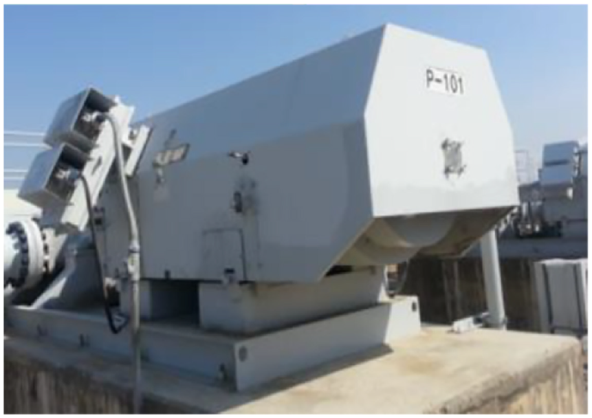
A hydrant pump in the fueling facility of an airport.
Development of degradation
Pumps are aging gradually in normal operations, but sometimes sudden degradation as a multi-state jump has been recorded in the maintenance log.
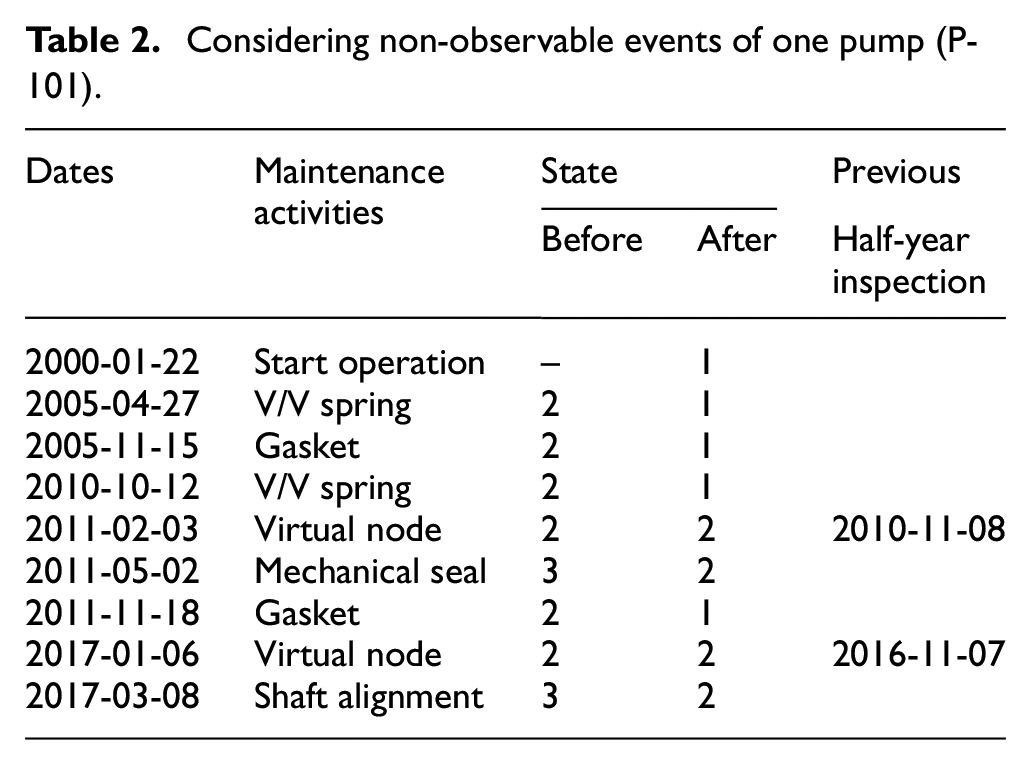
Periodic inspection is not perfect because the degradation level can be only known at inspection times, leading the jumps of observed system states. As a viable alternative, the pump should visit the intermediate states in the period from the last inspection until the event detection. The non-observable intermediate state will be placed in the middle of the period between the last half-year inspection and the current inspection of the event detection as shown in Table 2. With these procedures, the limitation of inspection is partly overcome by discovering various deterioration although defects can be only released at inspection time.
Considering non-observable events of one pump (P-101).
Modeling of degradation and CBM
The discrete state model is used in this study, and the empirical data provided has been already discretized.
Basics of Markov process
To clarify the symbols we use in the following analysis, some basics of Markov process are briefly presented in this subsection. The underlying assumption of the Markov process is the future degradation depends only on the current degradation state, known as memoryless property. A Markov process can be described as follows: assuming that


A sojourn time
The state probabilities are derived by the analytical solution of following equation in a matrix form:

Finally, to know the number of failures accounting for corrective maintenance, the number of the occurrence on the specific state can be outlined as
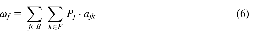
where the frequency
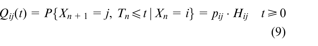
Modeling of inspections
A Markov process where the parameters and the state of the system can be changed at predefined points in time, such as when PM tasks are carried out, which causes alteration of transition matrix or the state in which the system is restarted.
10
When

By introducing maintenance decision matrix

where
Modeling of degradation and maintenance
Two more assumptions are needed in the degradation and maintenance progress:
Gradual degradation: A jump over two or more states is not possible. Therefore, the pump cannot skip the intermediate states where it is placed between two-state and intermediate states that have to be visited regardless of being explicitly revealed.
Minimal maintenance: Minimal maintenance means that the state of a system is restored just back to the previous state.
Here we use a SMP to model a degradation process. In a SMP, it is denoted that (1) the next state
where
1. Stage 1 (Transition Probability of EMC): Calculate the one-step transition probability matrix of EMC of SMP to obtain steady-state probabilities of EMC. It needs to consider the proportion of transition
where
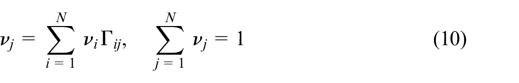
2. Stage 2 (Steady-State Probability of SMP): Calculate the sojourn time of each state in SMP model and computing steady-state probabilities of SMP using the steady-state probabilities of EMC and sojourn time.
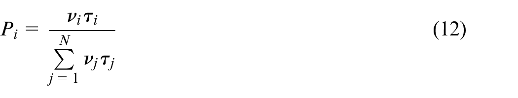
where
Equation (12) implies that the sojourn time has been represented by a mean value of an arbitrary distribution, which leads to the accuracy of estimating the mean sojourn time will play an important role in building SMP models.
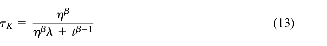
When the state does not has an exponential distribution for sojourn time to jump to other states, equation (4) is inapplicable. For the state
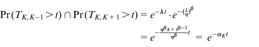
where
Empirical data analysis
The number of failures in the time horizon is of more interest in dealing with life data of repairable systems efficiently by treating it as a random variable, which is counting process. The goal of data analysis is to figure out the tendency of pumps status and identify transition rates toward deterioration direction for Markov model.
Counting process
Counting process takes into consideration a sequence of failure times. The main quantity is
Assuming an NHPP in (0,
The parameters are obtained by the partial derivatives (
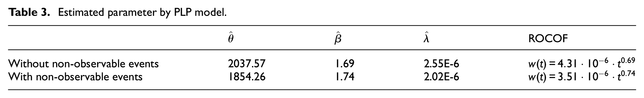
The estimated parameters are summarized in Table 3, and Figure 2 shows the Nelson-Aalen plot to illustrate the tendency. The resultant convex shape in the plots concludes the increasing ROCOF. The model with a non-observable state has a higher shape parameter that explains the reflection of the hidden non-observable events is closer to the real deterioration pertaining to the more rapid aging.
Estimated parameter by PLP model.
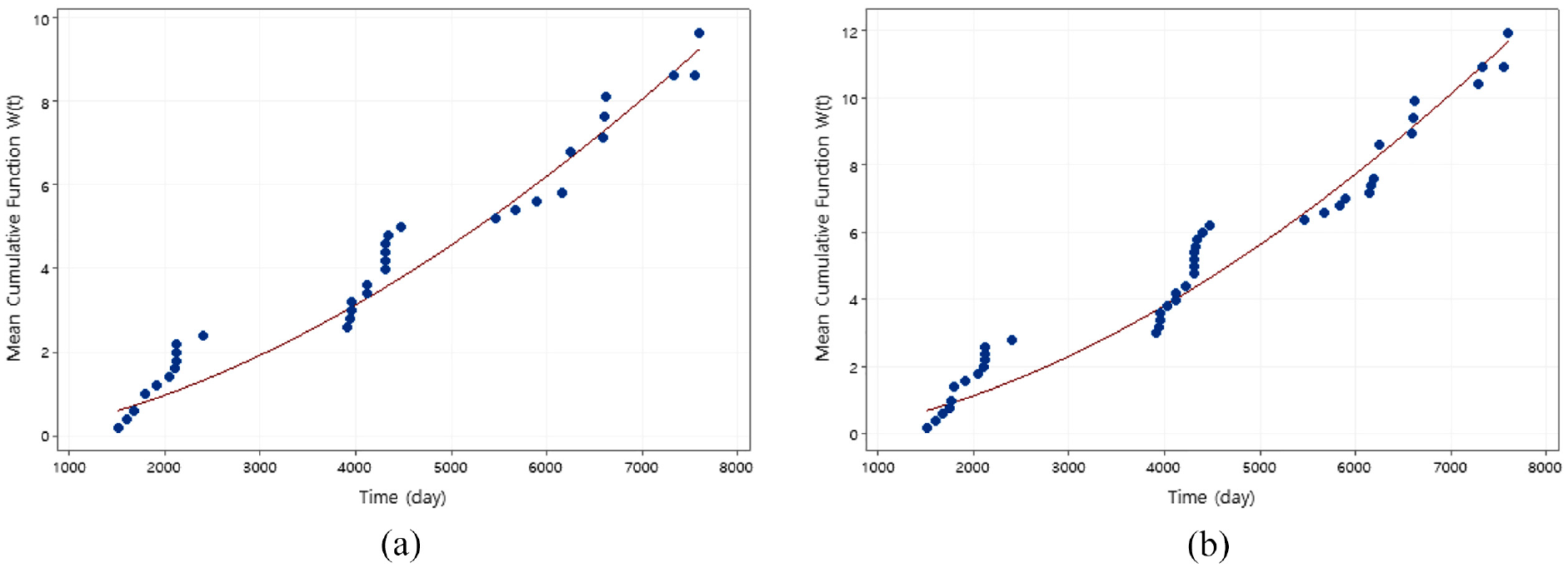
Nelson-Aalen plot: (a) without non-observable events and (b) with non-observable events.
Transition rates estimation
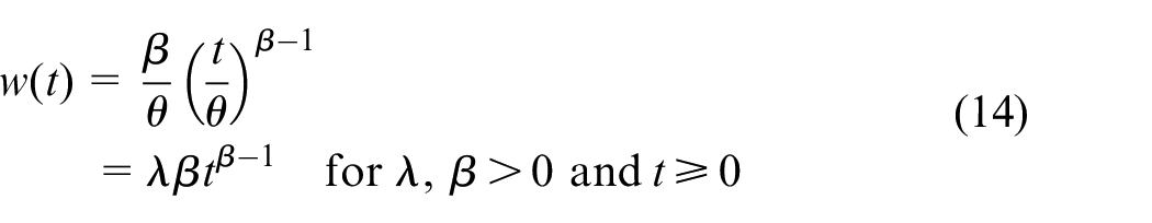
ROCOF of the NHPP built on global time is not a distribution technically. The modeling of the repairable system will undergo SMP central to local time, and the transition rates should be expressed by a distribution. MLE (Maximum Likelihood Estimation) is used for fitting the observable duration of each state expressed as exponential and Weibull distribution that is widely used in the industries.The estimated parameters shown in Table 4 for each law.
Estimated parameters.
(a) Exponential distribution.
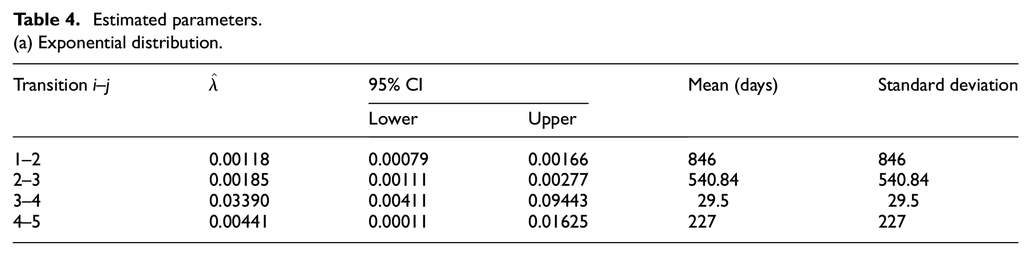
(b) Weibull distribution.
Numerical case studies
The following several conditions reflecting actual maintenance are mentioned before analysis:
Monthly inspection is conducted, but inspection frequency is highly increased from state 4.
Inspections take a short time, meaning pumps can be assumed available during inspection.
Repair is triggered at inspection dates without delays and lasts some random time.
Pumps are minimally maintained (PM), but it puts back as good as new when failed (CM).
A pump is not available during a repair.
Modeling and Monte Carlo simulation
We here consider the following situations with different considerations:
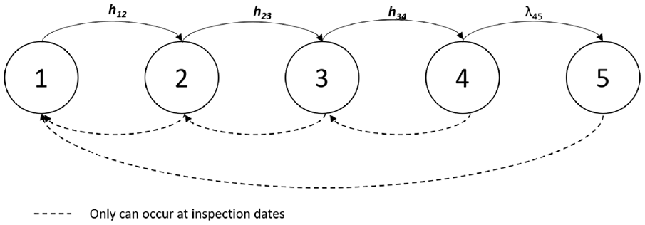
Homogeneous degradation with instantaneous maintenance: Regular inspections are conducted and transitions related to degradation follow exponential distribution. The proposed diagram for multi-phase Markov process is shown in Figure 3. This model can reflect the repair action but not the repair rate because the transition for backward jumps is not expressed as a distribution but instantaneous with the inspection.
Non-homogeneous degradation with instantaneous maintenance: The proposed diagram for SMP with instantaneous maintenance is shown in Figure 4. This model is the same as Multi-phase MP, except that the sojourn times have Weibull distribution in forward direction with time-dependent transition rates, but a constant rate of
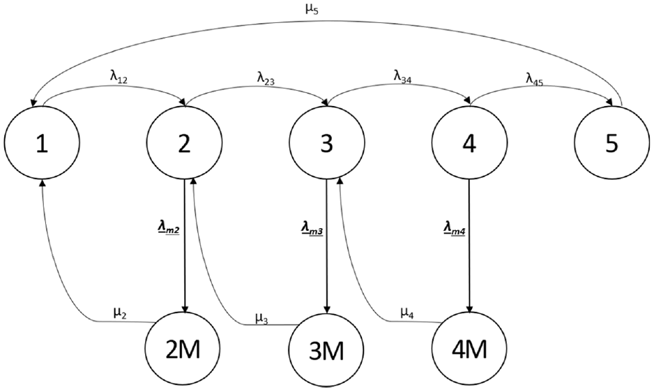
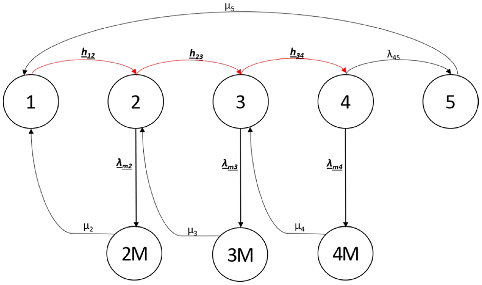
Non-homogeneous degradation with timed maintenance: To reflect time spent in maintenance, additional states to represent maintenance intervention to put back into the immediate previous state by repair. The corresponding graph is given on Figure 5, where 2M, 3M, and 4M are the states when the pump is under repair with rate
Monte Carlo simulation (MCS) with discrete event simulation is a powerful technique to overcome the complication of the analytical method. 11 MATLAB is formulated to do the simulation of 10,000 trials with a period of 20-year that refers to the median values for the life expectancy of based-mounted pumps from the equipment life expectancy chart of ASHRAE Handbook (2015). The step for one run of the simulation is depicted in Figure 6. For semi Markov process without repair rates, the algorithm is the same as Multi-phase MP except for adopting the Weibull random time generator.
Multiphase Markov model for homogeneous degradation with instantaneous maintenance.
SMP for non-homogeneous degradation with instantaneous maintenance.

SMP for non-homogeneous degradation with timed maintenance.
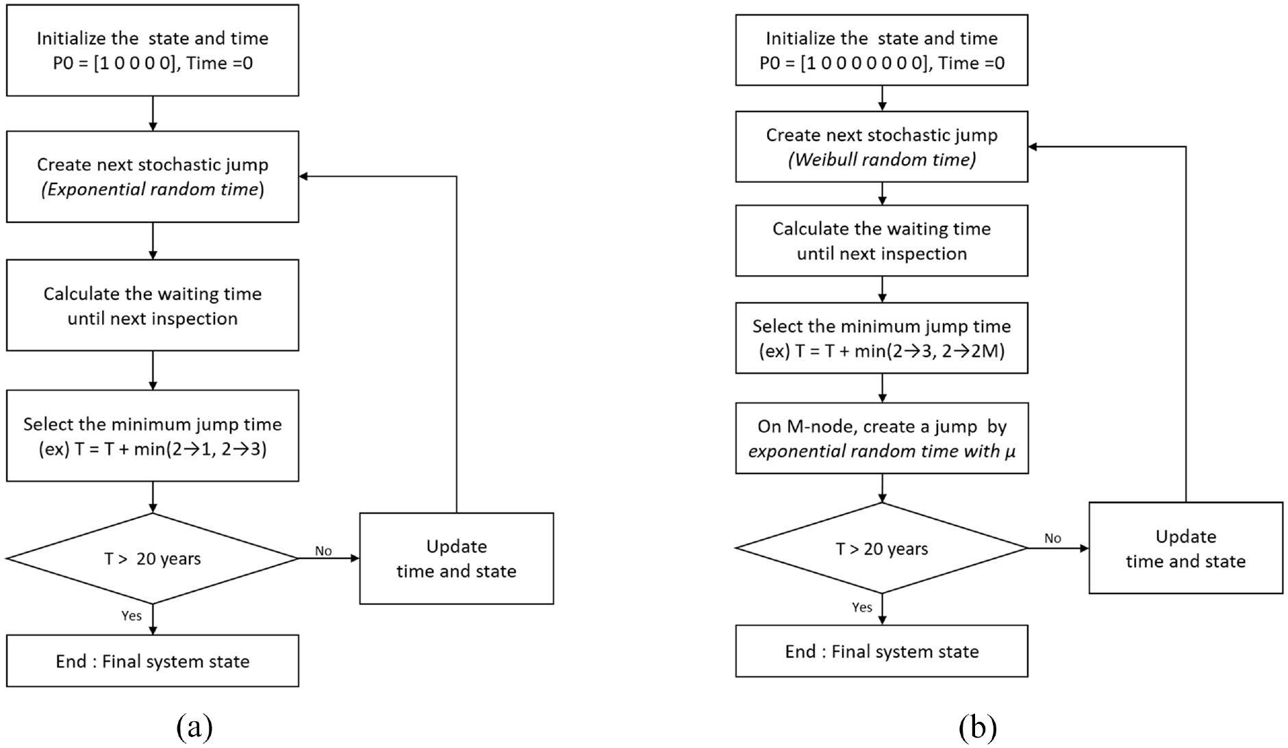
Flowchart of Monte-Carlo simulation with discrete event over 20 years: (a) multiphase Markov process and (b) SMP with repair rate.
Simulation results
According to Table 5, the dominant state of the pump in its life cycle is in state 1. Its availability is also relatively high, over 99.8%. The plot for comparison is outlined in Figure 7. This paper focuses on the probability for state 1, state 5, and availability to capture the mainstream about the status of pumps.
State probabilities computed by MCS.
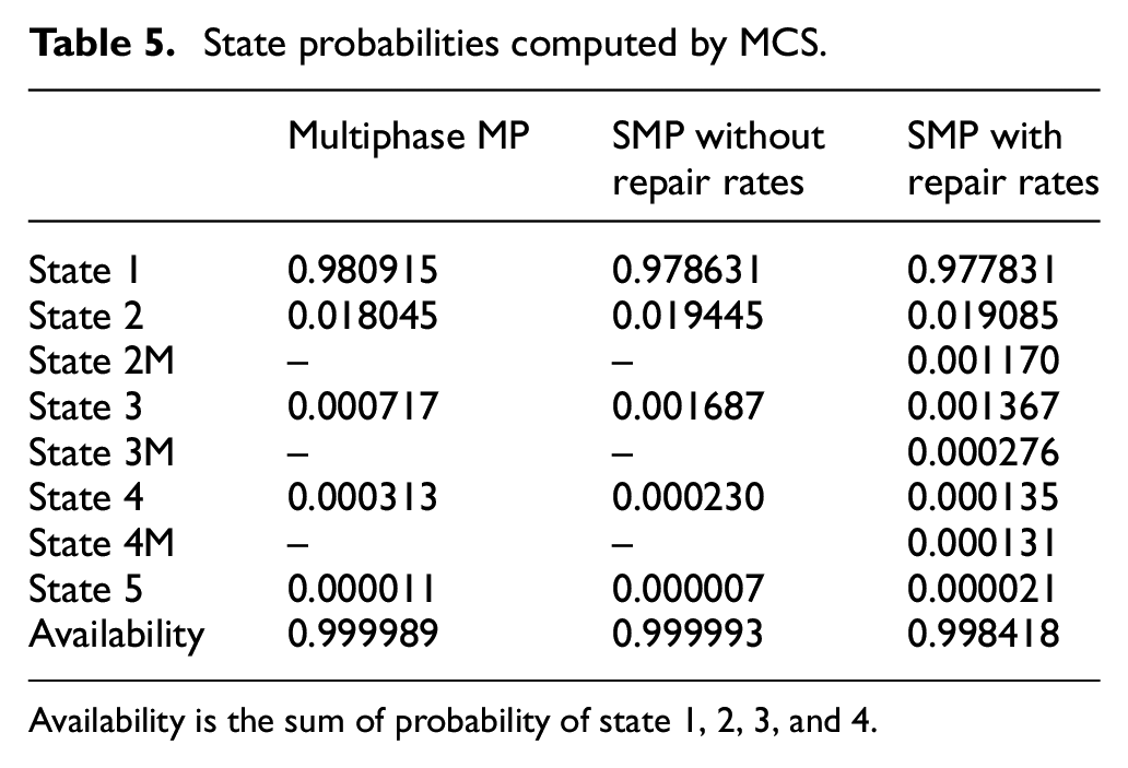
Availability is the sum of probability of state 1, 2, 3, and 4.
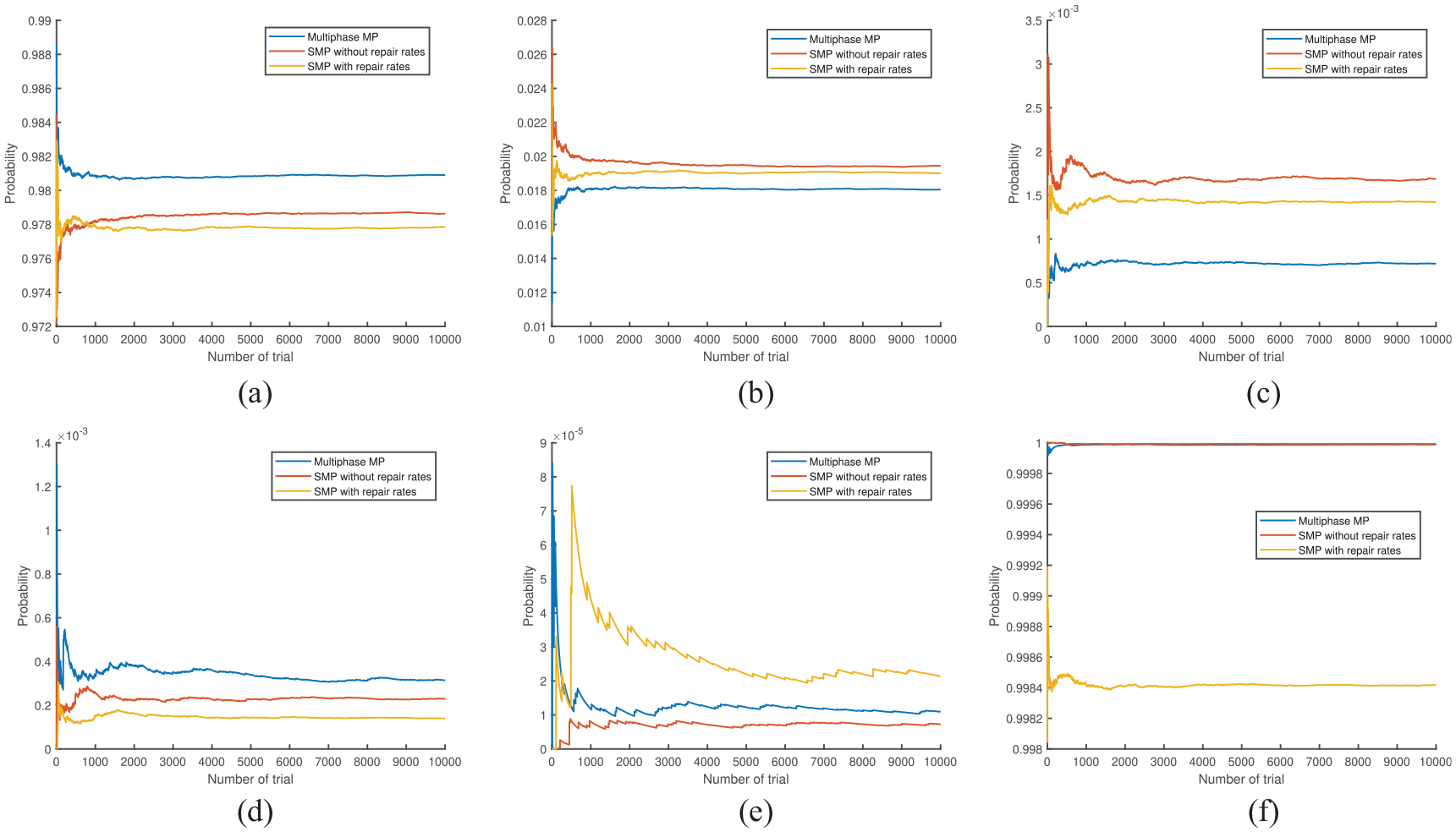
State probabilities computed by MCS under monthly inspection: (a) probability of state 1, (b) probability of state 2, (c) probability of state 3, (d) probability of state 4, (e) probability of state 5, and (f) availability.
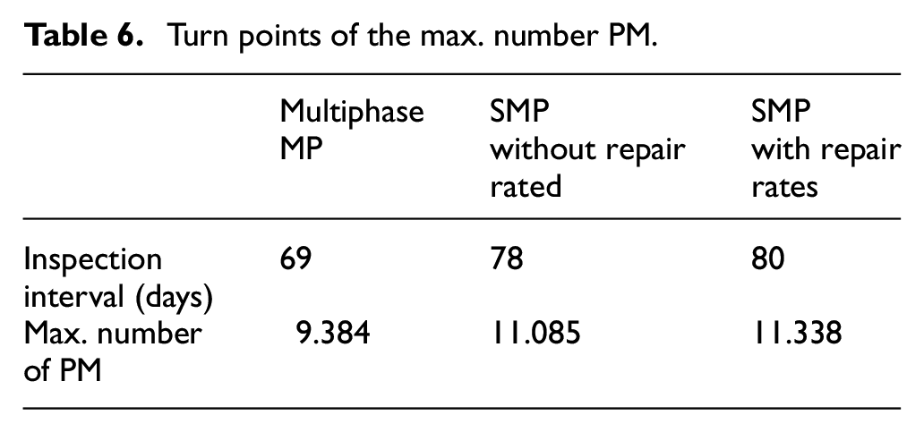
The next question is how the frequency of inspection influences the probabilities of state and the number of maintenance. It is argued that more frequent inspections can increase availability and reduce CM. Figure 8 gives a corresponding plot to capture the comparisons between Markov models to know explicit tendency. An effective indicator to demonstrate how close the prediction models are to reality is the number of PMs revealed in the maintenance log, which is 9.8 of the average number of PM for five pumps under monthly inspections. The multi-phase Markov process explicitly underpredicts the frequency of PM. However, the SMP model with the repair is a more realistic one not only availability but also the number of PM, compared to the actual record. It is interesting that PM increases until a specific interval and then decreases. The turn points driving the maximum number of PMs are shown in Table 6.
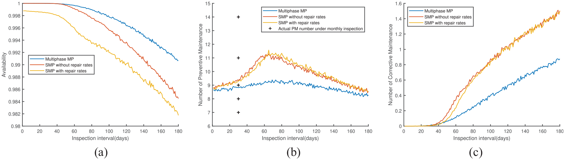
Probability and maintenance frequency with various inspection intervals: (a) availability, (b) number of PM, and (c) number of CM.
Turn points of the max. number PM.
Analytical approach
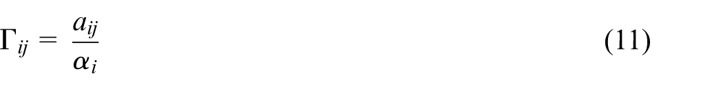
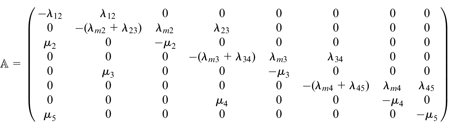
For the analytical solution, the first step is to calculate the transition probability matrix of EMC from CBM model. However, CBM model with periodic inspection stays far off from TCMC, and it also hampers the use of equation (8) inapplicable for the exponentially distributed sojourn times. This paper attempts to devise a procedure to build the Equivalent TCMC (E-TCMC) for allowing to use equation (11) that can compute transition probability matrix from its transition rate matrix.
Equivalent TCMC model
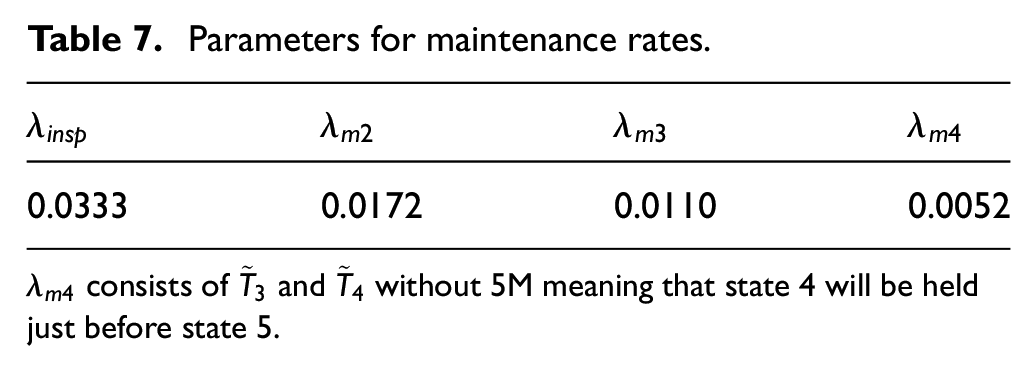
Because the timely maintenance is delayed due to waiting for the inspection, maintenance rate at state
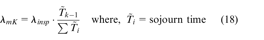
Equation (18) is derived from the idea that the longer sojourn times might correlate with a large amount of maintenance to return to its previous state. The maintenance rate,
Equivalent TCMC.
Parameters for maintenance rates.
Semi-Markov process model
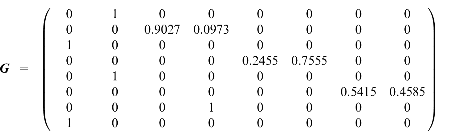
1. (Transition Probability Matrix of EMC) The transition rate matrix ( • State 1: (No. 1) the first row and column in the matrix • State 2: (No. 2) the second row and column in the matrix • State 2M: (No. 3) the third row and column in the matrix • State 3: (No. 4) the fourth row and column in the matrix • • State 5: (No. 8) the eighth row and column in the matrix
The steady-state probabilities of E-TCMC are outlined below.
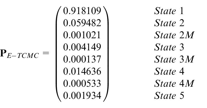
Consequently, equation (8) undertakes the computing task of the transition probability matrix (
2. (Steady-State Probability of SMP) It needs to change the transition rate from exponential to Weibull distribution to investigate SMP model corresponding to Figure 10. (a) (Proportion of Transition) It is possible to obtain the proportion of all transitions (
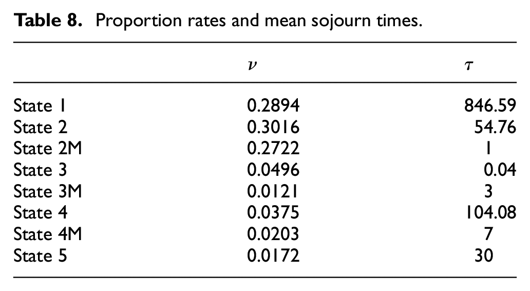
(b) (Steady-State Probability) Mean sojourn times can be computed using equation (13) for state 2 and state 3. Both the proportion rates (
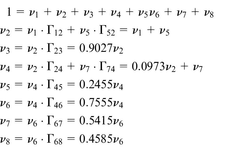
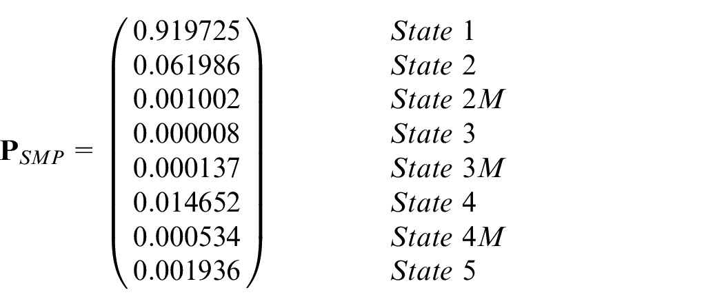
The steady-state probabilities of SMP,
Proportion rates and mean sojourn times.
SMP with maintenance rate
Comparison of the proposed models
A total of five models have been presented to find the state probabilities. The transition rate of SMP model allows the varying hazard rate to fit the model, but the multi-phase MP and E-TCMC have a constant transition rate. For this reason, SMP is preferable as its result is prone to be more comparable to actual data. It is claimed that the best fit model projecting the real-life of pumps is SMP with repair rates in numerical ways because there are few distortion and modeling errors. Therefore, it is a rational viewpoint to bring the result from that as a comparison criterion.
It is certain that the pump spends most of its life in lying good condition (state 1). It is noted that the equivalent models (E-TCMC and SMP using EMC) overpredict the derated state in skeptical manners markedly placed on state 4 and state 5, whereas state 1, good condition, is underestimated. This is possibly because the modeling error to proceed with approximation to
Illustration of optimal maintenance
This study seeks to find the optimal inspection interval that will give the lowest maintenance cost. E-TCMC model is used because it is straightforward and readily available with a constant transition rate. This study needs to come up with a factor, repair cost ratio (
Costs per inspection (
Costs per preventive maintenance (
Costs per corrective maintenance (
The objective function is intended to find the optimal inspection interval to bring the lowest asymptotic maintenance cost for the given period, as expressed in
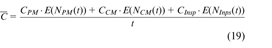
where
The optimal inspection interval for the 20-year operation is outlined in Figure 11 with repair cost ratio
Optimal inspection interval for 20 years operation: (a) maintenance cost, (b) optimal inspection interval, and (c) daily cost with
As discussed, these analyses can choose the best suitable strategies for several situations. With the aim of making the most of maintenance resources conducting multiple tasks simultaneously, inspection intervals requiring frequent PM, as shown in Table 6, might be avoided. When management puts weight on maximizing availability, inspection intervals should be shortened depicted in Figure 8, but on the other hand, minimizing the expected maintenance cost can be secured by the analysis outlined in Figure 11.
Conclusion and managerial implications
Conclusion
This paper has outlined a feasible approach based on the empirical data on hydrant pump maintenance. To identify the maintenance properties for CBM modeling, two frameworks are proposed in parallel: One is that the condition indicator is established in conjunction with repair activity itself. The other is how the hidden defects are considered in the gradual deterioration process by introducing virtual nodes when sudden degradation is observed, such as double jump without visiting intermediate state between departing and arriving state. The counting process is adopted to verify the degradation trend, and the distribution parameters are obtained by fitting the observed duration of each state.
The Markov models have been chosen for the CBM model regarding the probability of discrete state and the amount of maintenance.
Semi Markov Process is more accurate in predicting the degradation behavior by adopting the Weibull distribution, not constant rates as transition rates. Totally five models have been developed. SMP with repair rate using Monte-Carlo simulation model is the best fitting model to project the maintenance of the pump, computing 99.84% of availability and around 10 Preventive maintenance for 20 years. This paper attempts to solve analytically by establishing the reliable equivalent model transforming SMP including maintenance delay by inspection to TCMC, making it possible to obtain EMC of SMP. However, the reference model is not perfectly converted into the equivalent model due to approximation error to
Managerial implications
A periodic inspection is still of paramount importance to prevent degradation. This study suggests a framework to model the inspection-based maintenance utilizing Markov model to figure out the state probabilities, the amount of maintenance, and best inspection intervals. The managerial implications of the results and respective techniques are twofold. First, maintenance management can identify to determine optimum maintenance strategies minimizing the number of PM or the expected possible cost, thus deploying maintenance resources to maximize the overall benefit to the company. Second, CBM models can be built by continuously measuring physical properties to capture the item’s conditions, but it is not always possible. This study provides an indirect condition indicator using an inference framework for transforming work order data into state information when a direct condition indicator is not available.
Footnotes
Acknowledgements
We are very grateful to the anonymous reviewers whose comments have significantly improved the paper. We also would like to thank Yongjun Kim for allowing us to access the maintenance data of the system.
Declaration of conflicting interests
The author(s) declared no potential conflicts of interest with respect to the research, authorship, and/or publication of this article.
Funding
The author(s) disclosed receipt of the following financial support for the research, authorship, and/or publication of this article: The publication is supported by Norwegian University of Science and Technology, and Norwegian Agency for International Cooperation and Quality Enhancement in Higher Education (DIKU, Project No. UTF-2020-10099).