
Abstract
The failure processes of heterogeneous repairable systems with minimal repair assumption can be modelled by nonhomogeneous Poisson processes. One approach to describe an unobserved heterogeneity between systems is to multiply the intensity function by a positive random variable (frailty term) with a gamma distribution. This approach assumes that the relative frailty distribution among survivors is independent of age. Where systems are being continuously repaired and modified, the frailty distribution may be dependent on the system’s age. This paper investigates the application of the inverse Gaussian (IG) frailty model for modelling the failure processes of heterogeneous repairable systems. The IG frailty model, which combines the power law model and inverse Gaussian distribution, assumes that the relative frailty distribution among survivors becomes increasingly homogeneous over time. We develop the maximum likelihood for the IG frailty model, a method for event prediction, and investigate the effect of accuracy of the IG estimator and mis-specification of the frailty distribution through a simulation study. The mean estimates of the scale and shape parameters of the intensity function are examined for bias and efficiency loss. We find that the developed estimator is robust to changes in the input parameters for a relatively large sample sizes. We investigate the robustness of selecting an IG compared with a gamma frailty model. The developed IG model is applied to real data for illustration showing an improvement on existing models.
Keywords
Introduction
In the reliability literature, industrial systems are generally classified as either non-repairable or repairable.1,2 A non-repairable system is one where after a failure has occurred the system stops functioning and the system cannot be repaired. 2 A non-repairable system can fail only once, and a lifetime model such as the Kaplan-Meier, Exponential, or Weibull distribution provides the distribution of the time to failure of such systems. 2 A repairable system is a system that can repaired and returned to operation without the need to replace the system. 1
For repairable systems, we distinguish between the different system states after being repaired. 3 The system’s performance may return to the same state that it was at the start of operation, referred to as ‘as good as new’, or its performance may be returned to the same state as before the failure, that is, ‘as bad as old’ condition. 3 The former relates to a renewal process (RP) which is characterised by a renewal distribution describing the time between failures, and which is also called a perfect repair model, and corresponds to an assumption of the replacement of a system. ‘As bad as old’ condition can be modelled by a nonhomogeneous Poisson process (NHPP) which is characterised by the rate of occurrence of failures, and corresponds to the minimal repair assumption. 2 Minimal repair means that a failed system is restored just back to a functioning state, and after repair the system continues as ‘if nothing had happened’. 2 This implies that the likelihood of system failure, right after a failure and subsequent repair, is the same as it was immediately before the failure. Repair times in this kind of modelling are assumed to be negligible. 2
For many systems, the minimal repair assumption is appropriate to describe the maintenance regime adopted, that is, the purpose of repairing is to bring the system back to operation as soon as possible and the condition of the system is broadly the same as it was just before the failure occurred.3,4 For such systems, NHPP is a more appropriate model to characterise the failure occurrences in the systems than a renewal process. 3 NHPP models are flexible due to their assumption that events occur randomly in time, with rates which may vary with time. 2 NHPP allows the modelling of trends of the failure time occurrences such as whether a system is improving or deteriorating. 3 Therefore, this paper will concentrate on the modelling of repairable systems using NHPP.
NHPP are widely used models in reliability, for example: for analysis of failures of electrical power transformers in Dias De Oliveira et al. 5 ; for modelling of failures of ball bearing 6 ; for failures of numerically controlled machine tools in Wang and Yu 7 ; or for modelling software reliability. 8 NHPP have also been applied to other real world applications, that is, to study noise exposure in Guarnaccia et al. 9
This paper is concerned with the problem of predicting the behaviour of a system based on failure data from several similar systems. 2 According to Asfaw and Lindqvist, 2 Lindqvist 10 , Deep et al. 11 there may be unobserved heterogeneity among the systems which, if overlooked, may lead to inaccurate predictions. Heterogeneity among systems may be due to different material, different design, different location and so on12,13 while homogeneity among systems may be driven by similar repairing practises, similar usage patterns, etc. An intuitive way of interpreting heterogeneity is to imagine an unknown covariate, with values that may vary among systems, which leads to an unexpected variation in the failure intensity of the different processes. 3 The unobservable heterogeneity, which is often called frailty in the survival analysis literature, is typically modelled by multiplication of the intensity function by a positive random variable taking independent values across the systems with unit mean and therefore described by its variance. 3
The study of heterogeneity is widely applied in various fields like politics, 14 and medical research. 15 In survival analysis, the effects of unobserved heterogeneity have been studied in several papers including but not limited to Vaupel et al., 16 , Kheirietal., 17 Hanagal et al. 18 In reliability engineering, the effects of unobserved heterogeneity have been studied for various component problems like failures, 19 maintainability, 20 remaining useful life, 21 and spare-part management. 22 For non-repairable systems, some examples include Lin and AspLund 23,24, Linetal. 25 that used the frailty model to analyse the lifetime of locomotive wheels.
For repairable systems, unobserved heterogeneity has been studied with the minimal repair assumption. Early works include.26,27 Lindqvist et al. 28 developed a heterogeneous trend renewal process model, which generalises the HPP and NHPP, to capture unobserved heterogeneity in multiple repairable components. They introduced a gamma distributed multiplicative factor on the failure intensity. D’Andrea 29 suspected heterogeneity in the failure time data for mining trucks in Brazil. They assumed that the mining trucks were subject to minimal repair and thus modelled the data using NHPP with a gamma distributed frailty term.
Asfaw and Lindqvist 2 investigated heterogeneous population composed of independent NHPP using gamma-distributed frailty. Slimacek and Lindqvist 30 extended the basic NHPP to include covariates and unobserved heterogeneity in analysing wind turbine failure data. Lindqvist and Slimacek 3 developed the method for parameter estimations in heterogeneous NHPP population when the distribution of frailty is unspecified. The NHPP model was extended to include covariates in Slimacek and Lindqvist. 13 Most of these papers on minimal repair have parametrically modelled heterogeneity using the gamma frailty model in which unobserved effects are assumed to be gamma distributed.
Hougaard 31 introduced the inverse Gaussian (IG) distributions for modelling unobserved effects. The IG distribution has a unimodal density and is a member of the exponential family. Its shape resembles that of other skewed density functions, such as the lognormal and gamma distributions. Chhikara and Folks 32 studied the IG distribution and found that there are many striking similarities between the statistics derived from this distribution and those of the normal distribution. These properties make the IG potentially attractive for modelling purposes for survival data. 18
The IG distribution has some advantages as a frailty distribution. It provides flexibility in modelling, when early occurrences of failures are dominant in a life time distribution and its failure rate is expected to be non-monotonic. 18 Also IG is almost an increasing failure rate distribution when it is slightly skewed and hence is also applicable to describe lifetime distribution which is not dominated by early failures. 18 Hougaard 31 noted that survival models with gamma and IG frailties behave very differently, specifically that the relative frailty distribution among survivors is independent of age for the gamma, but becomes more homogeneous with time for the IG. The conclusion was derived by observing the coefficient of variation of the two frailty distributions of survivors. For the gamma distribution, the coefficient of variation is a constant. However, for the IG distribution, the coefficient of variation is a decreasing function of time. In fact, a few studies in areas such as medicine and epidemiology have suggested the IG frailty model as an alternative to the gamma frailty model for modelling unobserved effects.15,17,33,34
The likelihood function for the IG frailty model can be easily obtained and has closed-form representation, which indicates fast and simple estimation of parameters.18,35 Despite these desirable properties, for failure data with the minimal repair assumption, the application of the NHPP model in which the unobserved effects are assumed to be IG distributed has not be fully investigated. The first objective of this paper is to evaluate the application of the NHPP model with IG distributed frailties for analysing failure data from repairable systems and to compare its results with the gamma distributed frailties.
In a model with unobserved heterogeneity, it is necessary to define the distribution of the unobserved effects.36,37 Since the modelled heterogeneity is unobservable, the appropriate choice of distribution of the unobserved effects is not easily discernable.3,38 Furthermore, the choice of the distribution of unobserved effects can give interesting general results in terms of the variance of the unobserved effects). 3 For instance, a large variance could indicate deficiencies in the choice of the distribution which may influence the model fit.3,38 It is therefore useful to examine the extent to which mis-specification of the frailty distribution affects the validity of intensity function estimators. 38 Yet the impact of frailty distribution mis-specification with regards to the minimal repair assumption has not been investigated. Another objective of this paper is to examine the impact of wrongly specifying the frailty distribution in a NHPP model. To accomplish this objective, NHPP model with IG distributed frailties will be developed and compared with a gamma distributed frailty model through a simulation study and analysis of a real dataset. Statistical fit and prediction performance of the two models will be compared over different heterogeneity levels, sample sizes and component failure behaviours.
Another issue of interest in this paper pertains to event prediction for repairable systems subject to minimal repair and unobserved heterogeneity. The ability to predict the occurrence of failure events at an individual unit level can aid optimal maintenance decision making for individual components. 11 However, the majority of research on unobserved heterogeneity with the minimal repair assumption have predominantly focussed on investigating the significance of covariates and the frailty term in the fitted model rather than prediction for the system and/or individual components. The few works that have considered event prediction for point processes with unobserved heterogeneity includes: Deep et al. 11 that used a semi-parametric Andersen and Gill model for failure prediction of a new component in a Teleservice system using collected data from old units; and Jahani et al. 39 who developed a multivariate Gaussian convolution process (MGCP) for fleet-based event prediction in which failure prediction for an individual unit is conducted using data collected from other units. The third objective of this paper is to develop a method for predicting the occurrence of failure events at the component level based on the NHPP model with gamma and IG distributed unobserved heterogeniety effects. To accomplish this objective, an empirical Bayes framework will be adopted to update the frailty term.
The contribution of this study is threefold. First, we develop an IG frailty model and the parameter estimators for repairable systems whose components become homogeneous over time. Using a simulation study, we examine the performance of the estimators. Furthermore, we investigate the impact of mis-specifying the frailty distribution in a NHPP model. Finally, using empirical Bayes framework, we develop a method for prediction of a component’s mean residual life and prediction of the expected number of failures at the component and system levels.
The rest of the paper is organised as follows. First, we describe a general system with heterogeneous components. We develop the IG frailty model and an estimator for the IG frailty model. We describe a simulation study to investigate the accuracy of the estimator. This study is extended to further examine the impact of mis-specification of the frailty distribution. We present an analysis of a real dataset. We conclude by reflecting on the implications of our findings, the limitations of our study and provide suggestions for further work.
System description
Consider a system subject to minimal repairs upon failure. When a minimal repair is performed upon failure, the times between subsequent failures may not be identically distributed, which constitutes an NHPP.1,40
Consider that the system is a ‘happy system’ in its burn in phase. A ‘happy system’ has increasing inter-failure times. Also, consider that within a mission time, components in the wear-out phase (components with decreasing inter-failure times) are removed without replacement whereas components in the burn-in phase (relatively new components) are subject to minimal repair upon failure. As the number of the removed components increases, the relative frailty among the remaining working components in the system become homogeneous over time.
This paper shall concentrate on the most commonly used power law intensity function to characterise the ROCOF (Rate of occurrence of failures) of the NHPP (see e.g. Rausand and Hoyland
41
). One reason for its popularity is that the power law as a function of time

where
Consider that a system has m independent repairable components. Each component is observed from the start of operation to time
Conditional on the frailty term
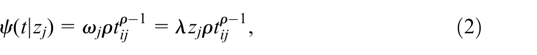
where
IG frailty model
This section presents an IG frailty model based on the NHPP with IG distributed random effects. IG distribution has a simple Laplace transform which is useful for deriving the reliability function.43,44 In addition, gamma and IG distributions both have uni-modal density functions.
44
IG distribution is described by two characteristics, namely, a mean parameter
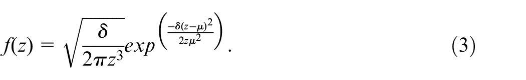
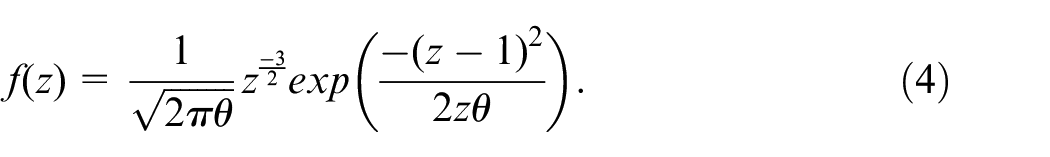
As mentioned above, the frailty model poses restrictions on the mean and variance on the distribution. Let
Maximum likelihood for IG frailty model
Assume that the random effect
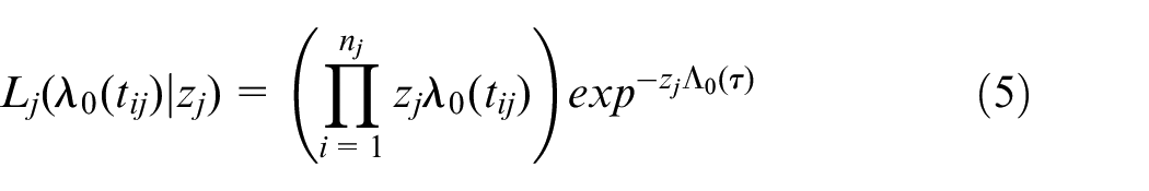
where
The total log likelihood function for all the components is given by:
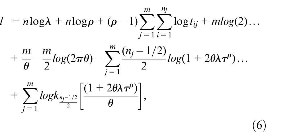
where
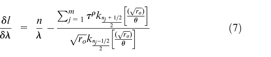
where
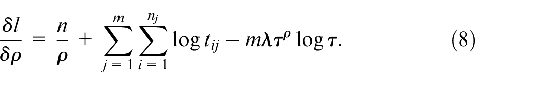
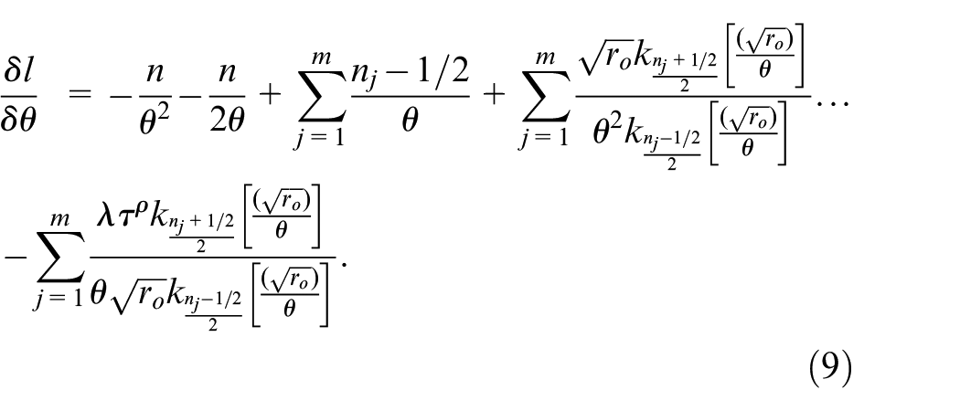
Estimates of
Simulation study
In this section, we conduct a simulation study. We describe the simulation design and data simulated. We assess the performance of the IG estimators with respect to bias in the estimates of the scale
Simulation design
Throughout the simulation study, the underlying failure process for the components in a system are considered to follow a nonhomogeneous Poisson process (NHPP) with basic rate of occurrence of failures of a power law process
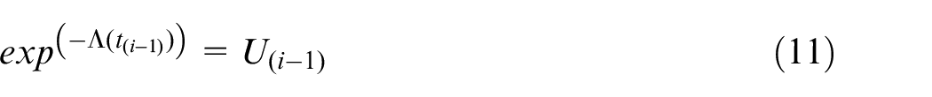
To perform the simulation study, data is generated. The following algorithm is used to generate failure time data from each frailty model. If the failure times of a component are assumed to be independent given the frailty term and that the sequence of failure times forms a counting process, samples of an NHPP can be generated from an Homogeneous Poisson Process (HPP). Consider an HPP with intensity function

where the random variables
and

where

where

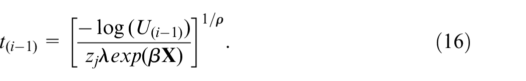
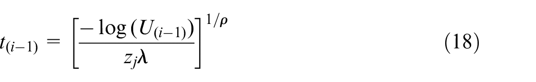
Solving for a failure time
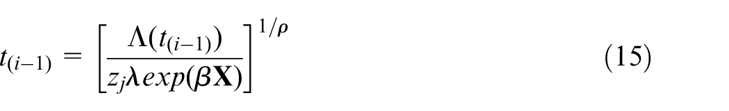
and
The NHPP process of component j observed up to the
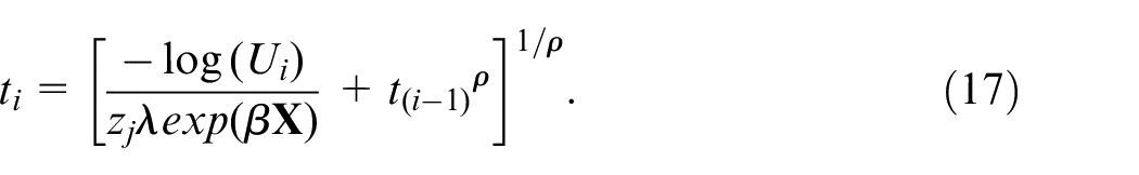
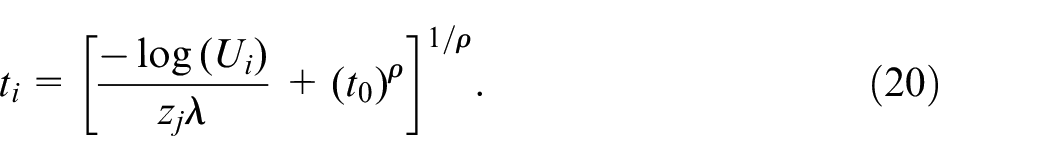
If there are no available covariates that is,
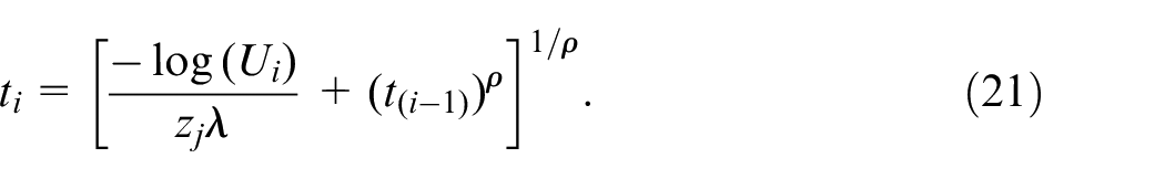
and the recurrence formula becomes

To illustrate how to generate data when covariates are unavailable, a single NHPP process for component j can be simulated by the recurrence formula in equation (19) using the algorithm below.
Set parameter values for
Set a value for
Draw a random value
Set
Set
Draw
Generate the first failure time by:
8. If
9. Draw
10. Generate the next failure time as:
11. Repeat steps 8–10 until
Evaluation of IG estimator
To assess the performance of the IG frailty model’s estimator developed earlier in this paper, the Bias
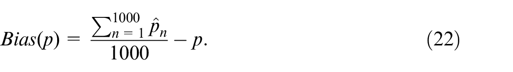
We assess the IG estimators by observing the
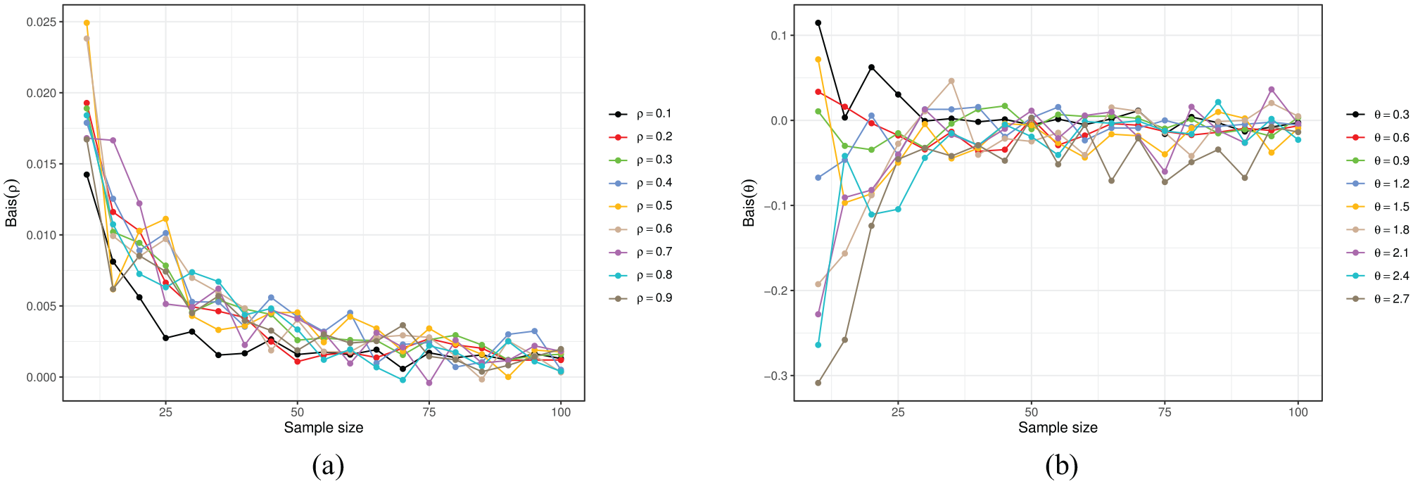
Plot of the Bias on estimates from IG frailty model estimators: (a) bias on ρ input values and (b) bias on θ input values.
From Figure 1(a) we observe that the bias in the estimated
Mis-specification study of gamma and IG frailty models
In this section, we assess the performance of the gamma and IG estimators to mis-specification of the frailty distribution. When one of the models is known to be the correct frailty model from which the data are generated, and the other frailty model will in consequence be wrongly specified. The performance of the wrongly specified model will be assessed in terms of the model’s goodness of fit to the generated data and prediction accuracy when predicting the expected number of component failures. Since model selection using only maximum likelihood could be misleading due to variation in data, the sample sizes will be chosen to be sufficiently large in order to reduce the probability of selecting the wrong model. 45
Analysis of the robustness of each wrongly specified frailty model (gamma or IG) is conducted by an assessment of the proportion of selections of each wrongly specified model using Akaike information criterion (AIC). AIC is used for goodness-off fit (GOF) test because AIC is one of the commonly used information-based criteria for model selection 46 and the AIC has been widely used either on its own or together with other tests (e.g. Barabadi et al., 22 Izumi and Ohtaki 47 ). AIC is similar to the Bayesian information criterion (BIC) in the sense that they both compare maximum likelihood values to select the appropriate model. Compared to AIC, BIC penalises model complexity more heavily meaning that more complex models will perform worse and will, in turn, be less likely to be selected. 48 In this paper, the Gamma and IG frailty models considered have the same number of parameters and similar level of complexity. Thus, model selections from BIC will not differ from AIC because the penalty term in the BIC will have the same effect on the two model’s values. AIC has been widely used to compare frailty models in the literature some examples include.49,50 The expression of AIC is given by 46 :

where
Furthermore, we examine the robustness of each wrongly specified frailty model in terms of their prediction of the expected number of component failures in the simulated data. The expected number of component failures in the system in a specific interval is given as:
where
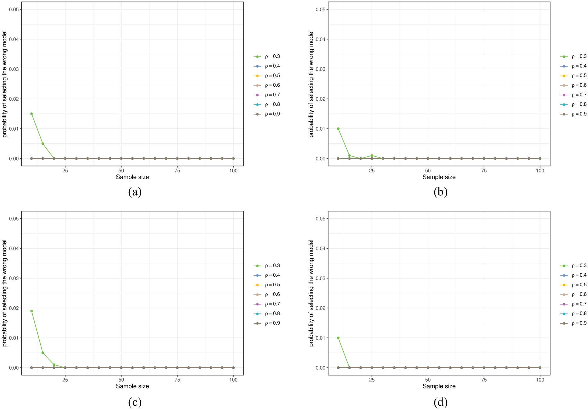
We compare the predicted results with those from the correct model using root mean squared error (RMSE). We then assess the proportion of the wrong model selected as the better model by the RMSE. The expression of RMSE is given by:
where
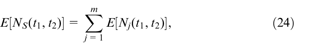
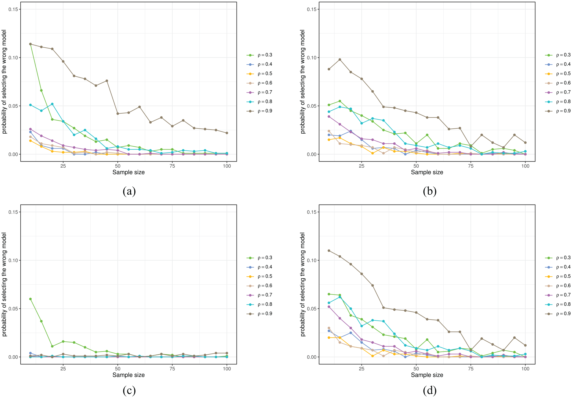
The performance of each specified model is assessed in four cases involving fixed
Case one involves setting
Case two involves setting
Case three involves setting
Case four involves setting
In each case, when one of the two parameters is fixed, the other is varied. For fixed settings of
Plot of probability of selecting the wrong model when heterogeneity is low
Plot of probability of selecting the wrong model when heterogeneity is high
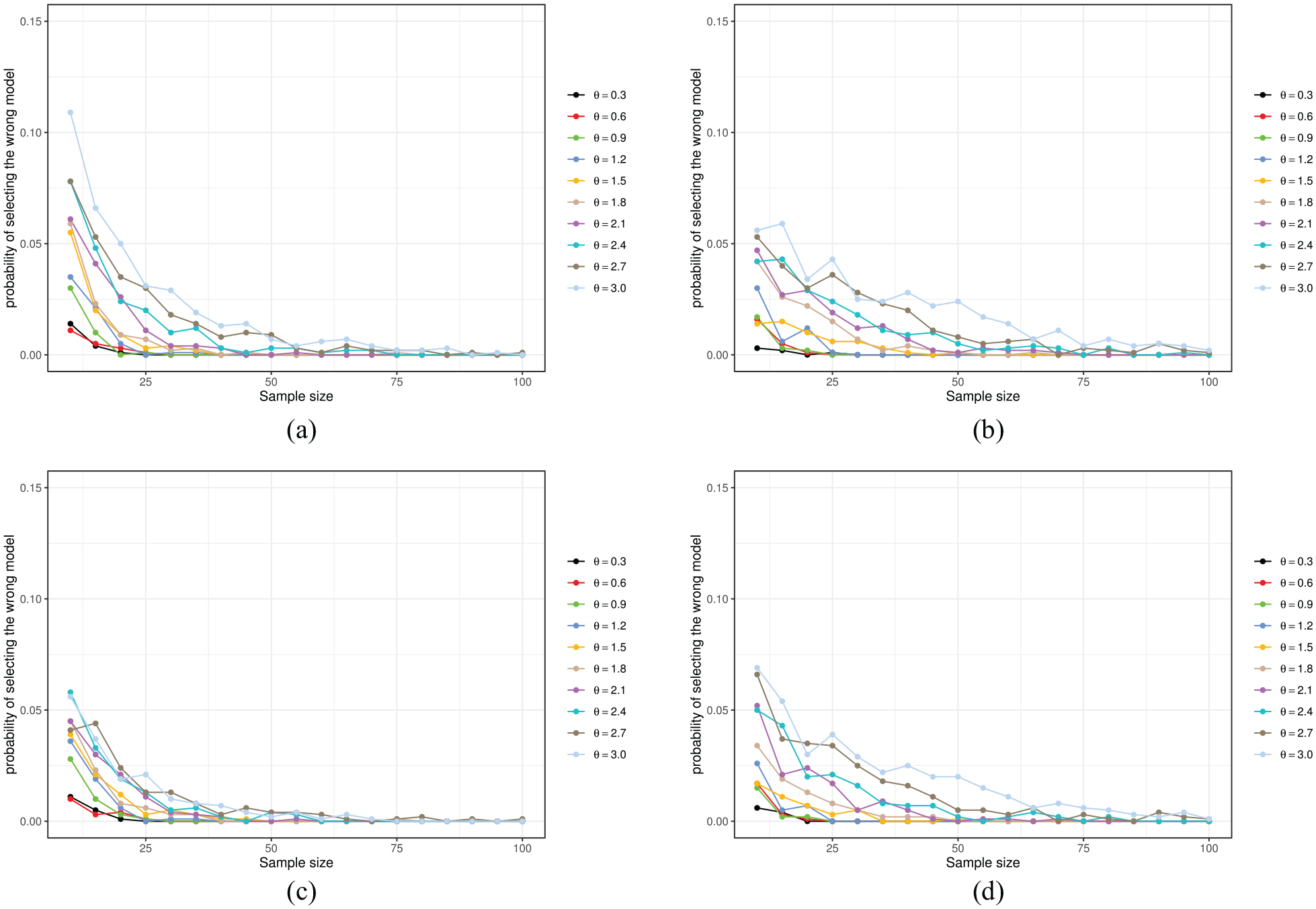
Plot of probability of selecting the wrong model when early life failures are considered
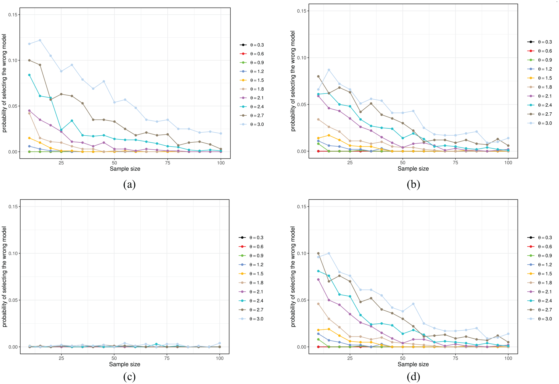
Plot of probability of selecting the wrong model when component failures are similar to the mid-life phase
Case One: Low heterogeneity
In case one, we set
Case Two: High heterogeneity
For case two, we set
The results for determining the appropriate model when using prediction as the measurement are presented in Figure 3(c) and (d). We observe a similar reduction in incorrectly selected models when gamma is wrongly specified. When IG is wrongly specified, the proportion of IG model selection is zero for
Case Three: Component early life behaviour
In case three, we set
Case Four: Component mid-life behaviour
In case four, we set
Summary of analysis
Reflecting on our study, several conclusions can be drawn from our analysis. First, when the sample sizes increase above 50, the likelihood of selecting the wrong model significantly reduces for almost all choice of parameters. This provides confidence that when we have many units/components, we are likely to select the correct model. Second, the effect of heterogeneity for low sample sizes is noticeable. As we increase the heterogeneity from
Application to classic dataset
We compare the two frailty models using a dataset from the literature, that is, failure times of air conditioner components from a set of airplanes studied by. 28 This data was used as 28 compared a Heterogenous trend renewal process, an NHPP model with gamma distributed random effect, and a Homogeneous Poisson process with gamma distributed random effect. Lindqvist 28 found that an NHPP model with gamma distributed random effect provides a better fit than Ordinary NHPP model, identifying heterogeneity among components in the data. Here we compare the IG and gamma frailty models using the successive failure times before truncation as given in Table 1 to see if the IG provides a better fit. Note that it is not possible to say whether or not the true data generating process comes from an IG or Gamma; we merely wish to explore if our model produces any improvements on existing methods.
Failures times for Air conditioners in 13 Airplanes.
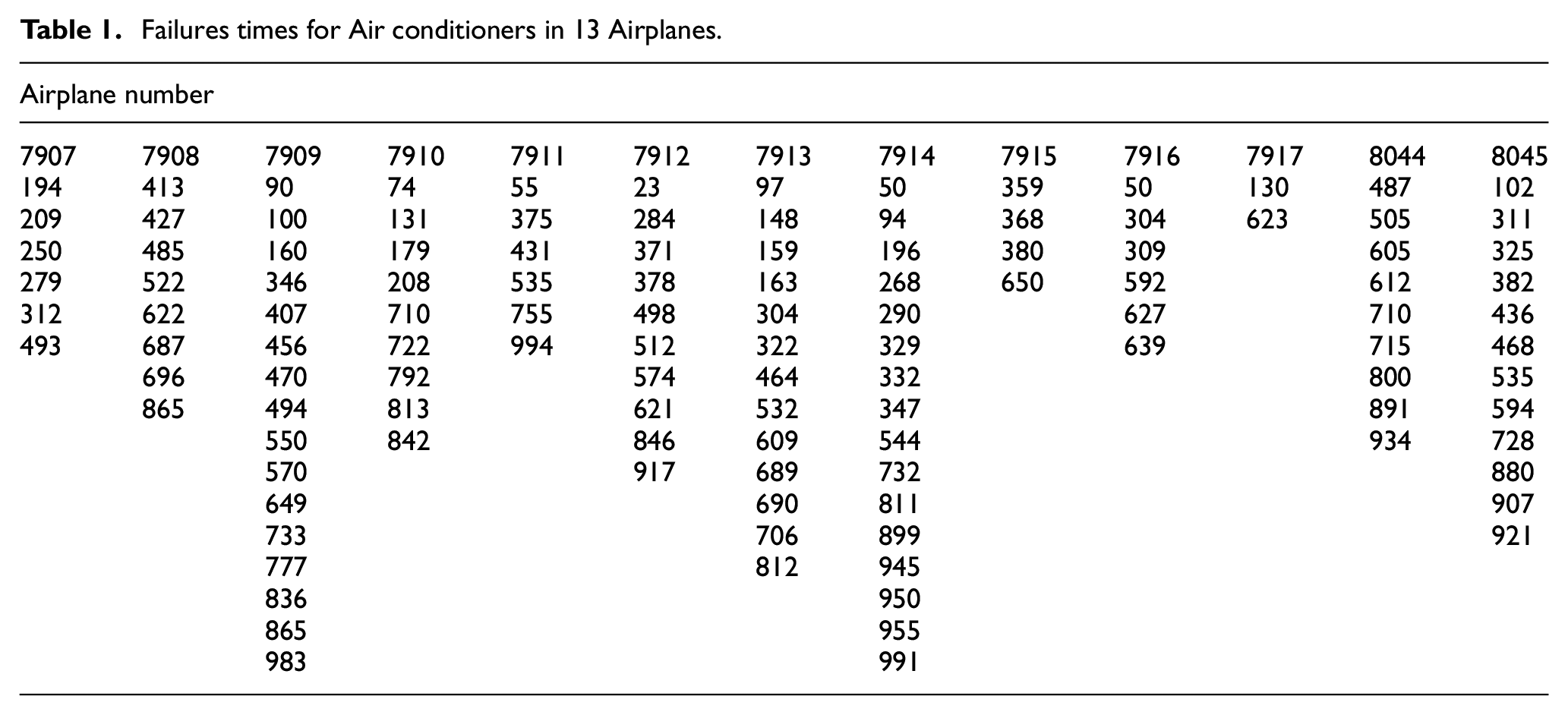
The results of fitting IG frailty model and gamma frailty model are summarised in Table 2. Parameter estimates for the gamma frailty model were obtained as
Parameter estimates of gamma and IG frailty models when fitted to Air conditioner failure time data.
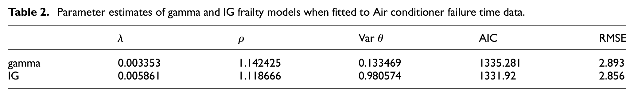
Furthermore, we compared predictions of the expected number of failures from the two models with observed data using RMSE. We found that there is little difference in the predictions of the observed number of system failures from the gamma and IG frailty models when time is less than 500 days (see Figure 6 for the plot of the predictions). However, in line with Hougaard 31 findings that the relative frailty distribution among survivors from an IG model becomes more homogeneous with time, we found that once we extend beyond 500 days the survivors become more homogeneous and the IG model substantially outperforms the gamma. Based on the selection values of AIC and RMSE in terms of model fit and prediction, one can infer that IG frailty model is marginally better in terms of model fit and better in terms of predictions of the expected number of component failures for the air conditioner data when number of days is greater than 500.
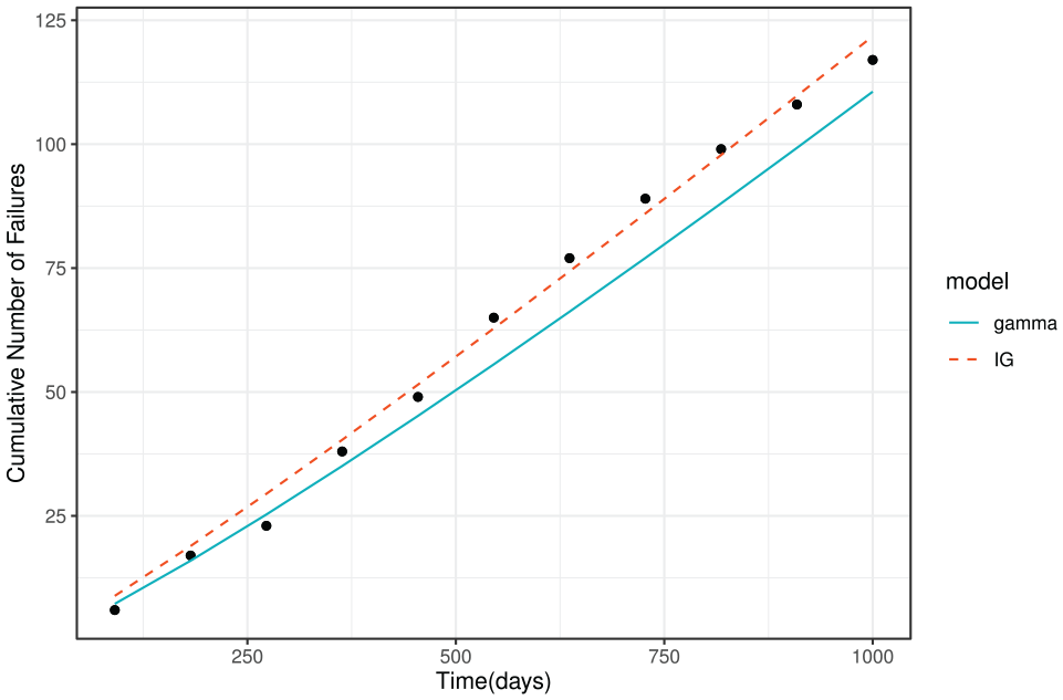
Plot of the expected number of failures predicted by the IG and gamma frailty models compared to the observed cumulative number of failures within the interval 0–1000 h (system level prediction).
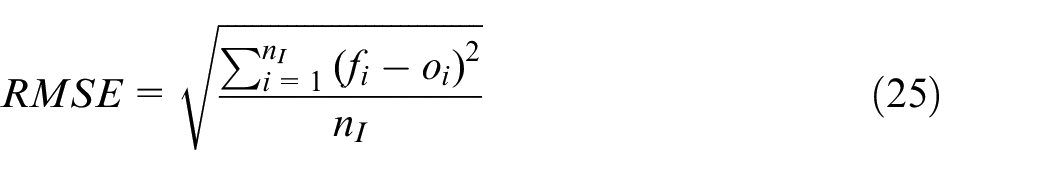
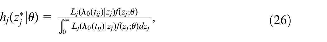
Equation (24) is useful for predicting the expected number of failures at the system level. For component level prediction, the predicted number of failures for all the components will always be the same, even if there are clear differences in the pattern of failure occurrences. The reason is that the value of the variance parameter
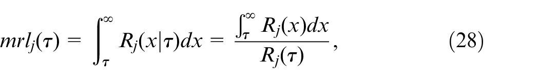
Using an empirical Bayes approach, we developed a method for individual component prediction of the mean residual life (MRL) and expected number of failures conditional on the expected frailty value. The developed method is then applied to make predictions for components in the Air conditioner data. The developed method uses Bayes theorem to update the frailty distribution for each
Using Bayes theorem, we can have the posterior distribution of the frailty term
where
The expected number of failures of the
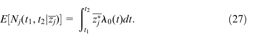
System level prediction of expected number of component failures is
where
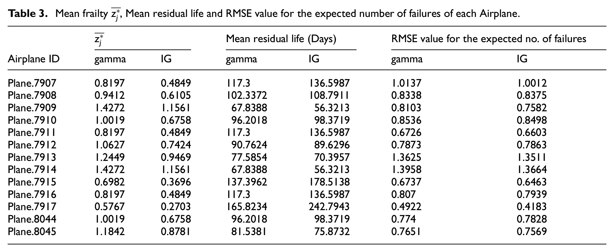
For each of the components (Airplanes) in the Air conditioner data, we predicted the mean residual life and compared predictions of the expected number of failures from the IG and Gamma models with observed data using RMSE. The mean frailty estimate for each component
Mean frailty
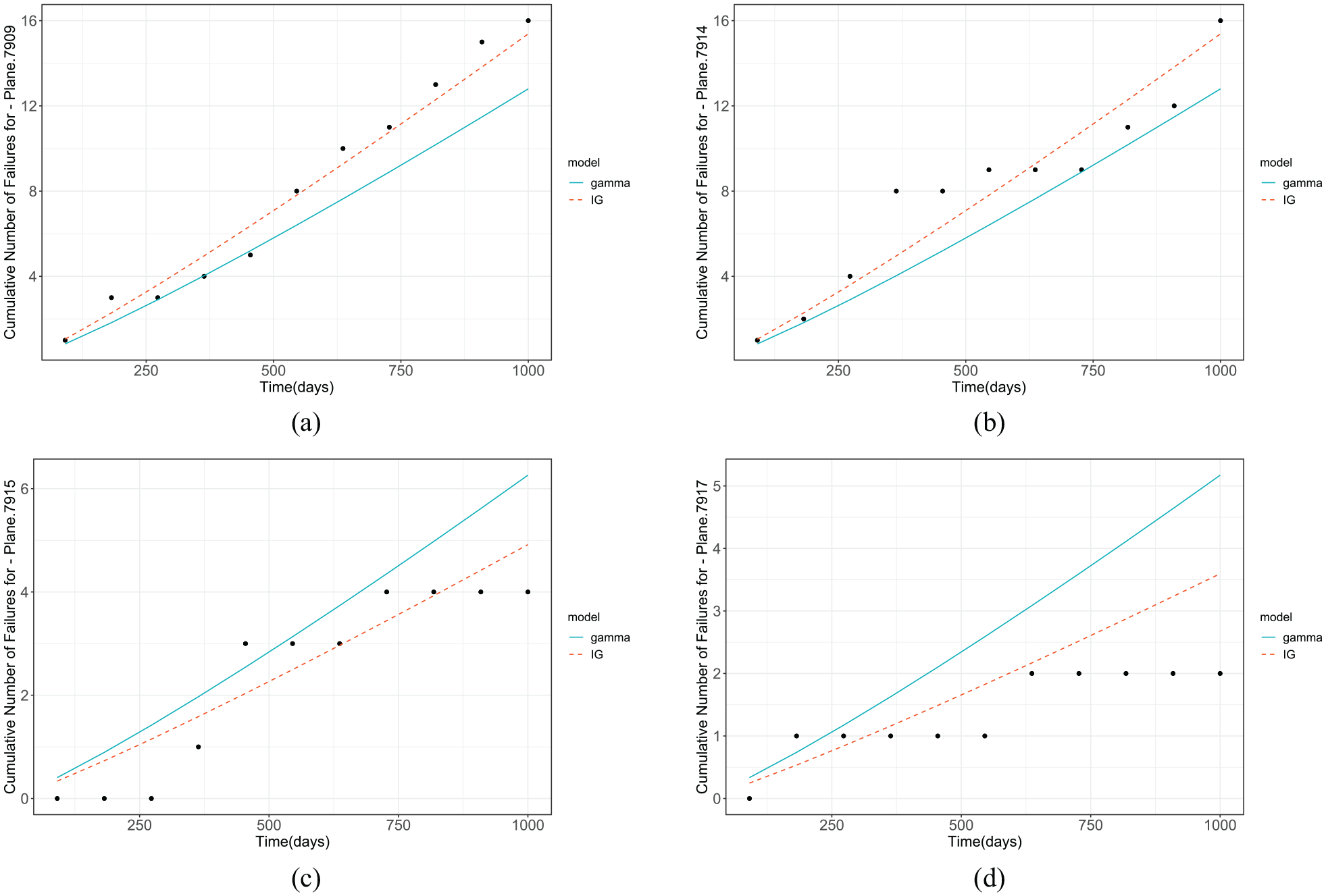
Plot of the expected number of failures predicted by the IG and gamma frailty models compared to the observed cumulative number of failures within the interval 0–1000 h (component level prediction): (a) Airplane 7909, (b) Airplane 7914, (c) Airplane 7915 and (d) Airplane 7917.
In terms of mean residual life predictions for each component Airplane, we apply Eq 28 for IG and gamma frailty models and found that there are differences in the MRL predictions of the Airplanes by the two models. For some Airplanes, for example Airplanes 7910, 7912 and 8044, the difference was as little as one or 2 days. In other Airplanes such as: 7909, 7911, 7913, 7914, 7915, 7916 and 7917, the differences ranged from eleven to 77 days. However, given the selection of the IG frailty by the RMSE values of a lot of the Airplanes, the MRL predicted values by the IG frailty model may be chosen for optimal maintenance decision making for most of the Airplanes.
Conclusion
In this paper, we applied the IG frailty model for analysing failure data from heterogeneous repairable systems. The IG frailty model, which combines the power law model and IG distribution, assumes that the relative frailty distribution among survivors becomes more homogeneous over time. This is in contrast to the commonly used gamma frailty models which assume that the relative frailty distribution among survivors is independent of age. The objectives of this paper were to evaluate the application of IG frailty model for analysing failure data from heterogeneous repairable systems, compare its results with the gamma frailty model, and develop a method for event prediction based on the IG and gamma frailty models. To accomplish the objectives, we developed the IG frailty model and a method for parameter estimation of the IG frailty model using maximum likelihood estimation and numerical methods. A comparison of the gamma and IG frailty models was conducted to examine whether both models are good alternatives of each other. Statistical fit of the gamma and IG frailty models as well as the prediction performance was thoroughly studied and compared. We found that regardless of the degree of heterogeneity or frequency of failures when early component behaviour is concerned, the probability of selecting a wrong model is low whether for model fit or for prediction purpose. A wrong model is only selected when the sample size is small. We applied the two frailty models to a classic dataset where the gamma frailty model had been studied. Our results found that the IG frailty model was better in terms of model fit and prediction when the number of days was greater than 500.
This research identified a number of areas for future research. First, the IG frailty model could be integrated into other degradation processes to explore its advances more broadly in reliability modelling. Instead of using the Gaussian or gamma distributions, further research could investigate other positive skewed distribution to describe unobserved heterogeneity. In addition, it would be valuable to further investigate the application of the IG frailty model. For example, when a system is operating in a varying environment, its degradation parameters are usually random and dependent on the operating environment, which can be potentially characterised by the IG frailty model. Another interesting research direction lies in the way of describing uncertainty in reliability modelling. Instead of using a probability distribution, fuzzy sets or interval values could be used to model the uncertain parameters or coefficients.
Footnotes
Appendix A
The derivation of the IG frailty model’s unconditional log likelihood function is presented below.
Since
where
The marginal likelihood of the
where
The total likelihood function for all the components is given by:
Taking the logarithm of the likelihood function of equation (32) results in:
Appendix B
The expressions for the posterior distribution, expected frailty value, expected number of failures and marginal reliability function for the IG frailty model is derived as follows.
The marginal reliability function of the
where
and
where
The marginal expected number of failures of the
The marginal expected number of component failures in the system between time
where m is the number of components in the system.
Next we derive the posterior distribution for
The value of the frailty term for component
Then
and
where
Appendix C
The expressions for the posterior distribution, expected frailty value, expected number of failures and marginal reliability function for the gamma frailty model is derived as follows.
The marginal reliability function of the
where
Thus,
and
where
The expected number of failures of the
The expected number of component failures in the system between time
where m is the number of components in the system.
Next we derive the posterior distribution for
Replacing the expressions of
The expression for the mean of the updated frailty distribution
However,
where
Declaration of conflicting interests
The author(s) declared no potential conflicts of interest with respect to the research, authorship, and/or publication of this article.
Funding
The author(s) received no financial support for the research, authorship, and/or publication of this article.