
Abstract
The Indian Premier League is the most prestigious cricket league globally. There are significant finances in terms of both team ownership and player salaries. It is, therefore, essential to understanding if a team’s record is due to luck (good or bad) or if a team’s record is due to the team’s overall performance. The research presented here is motivated by how to accurately predict a team’s winning percentage in the Indian Premier League based on underlying statistics. A similar analysis has been done in other sports, mainly based on the concept of the Pythagorean expectation. This research derives a similar model for the IPL based on historical data. However, the structure of a match in the Indian Premier League is fundamentally different than the structure of games in other sports. As a result of this structural difference, this study creates additional models using both least absolute shrinkage and selection operator and stepwise regression to identify variables that are good predictors for calculating the expected winning percentage. These models compare favorably to the Pythagorean expectation model. This article presents a model combining both the determined variables and Pythagorean expectation.
Introduction
The game of cricket is a bat-and-ball game where the objective is to score more runs than the opposing team. Cricket is among the most popular sports globally, with viewership second only to football/soccer. The world’s most financially lucrative cricket league is the Indian Premier League (IPL); in 2019, the value of the IPL was over US$6 billion. This research investigates the calculation of the expected winning percentage of a team during a season based on their underlying statistics. The format of T20 cricket played by the IPL differs from other sports. For most other sports, a clock controls the game’s length. In cricket, there is no clock, so the game ends after each team has completed their overs rather than the clock expiring. However, there is an additional significant difference between cricket and other sports concerning the change from offense to defense. In most sports, teams continually shift between offense and defense as possession of the ball changes. For cricket, there is a single change between offense and defense.
As will be seen in the literature review, there has been substantial work investigating baseball winning percentages. Baseball has many similarities to cricket (both sports have similar origins). For example, both are bat-and-ball games and do not involve a clock. However, the switch from offense to defense is significantly different between the two sports. Each team has 27 outs in baseball, with the outs split up into three-out innings. In a baseball game, one team has three outs, then the teams switch from offense to defense, and the second team gets three outs. The process repeats until all 27 outs have been utilized. In T20 cricket, one team utilizes all of its overs, and then there is a single instance where the teams switch from offense to defense. In baseball and T20 cricket, if one team has no offensive opportunities left and has a lower score, the game ends without playing out the remaining opportunities. In baseball, this is not as significant of concern because, at most, three outs are not played, and, based on the average rate of scoring, less than one run would be scored by the team during the skipped offensive opportunities. A more significant percentage of the total number of overs could go unplayed, and the scoring rate per over is substantially >1. Based on the data for this article, an average of 17.8 overs per game are played out of the 20 possible overs. As shown later, this single switch from offense to defense provides a challenge in evaluation that is not seen in other sports because the total score is not as significant as the scoring rate.
Literature review
As both sports analytics and the size of the IPL grows, the amount of academic literature is also increasing. While not directly related to team performance, research has investigated the efficiency of spending by IPL franchises. Singh 1 uses data envelopment analysis (DEA) to measure the technical efficiency of spending versus performance. Jana et al. 2 use DEA and structural equation modeling (SEM) to perform a similar analysis.
Several researchers have applied machine learning techniques to predict the winner of a match immediately before the match commences. Nimmagadda et al. 3 implement a random forest algorithm to predict the winner of the match based on predicted scores determined using multiple variable regression and logistic regression. Kapadia et al. 4 use filter methods to identify key features and then use this data to solve the classification problem of which team will win. Raja et al. 5 use machine learning techniques to predict player performance and use these estimates to solve the classification problem of the winner of the match. Jayanth et al. 6 use support vector machines (SVM) to predict the winner of a match by grouping players at different levels in the batting order. While not explicitly applied to the IPL, Wickramasinghe 7 uses a Naive Bayes approach to predict the winners of a One Day International (ODI) cricket match. Bhattacharjee and Talukdar 8 investigate the application of discriminant analysis using a defined pressure index. Their cross-validated results show good predictive performance.
In addition to building a model for predicting match winners, Singh and Kaur 9 and Raviteja et al. 10 both, in addition, perform data visualization to help show player performance in addition to predicting the winner and loser of the match. Tekade et al. 11 use different supervised machine learning outcomes to predict the result of a match. Similarly, Vistro et al. 12 use machine learning algorithms to predict the winner before the match begins. Tripathi et al. 13 also predict the winner of a single match but have the added contribution of solving multicollinearity issues. Sinha et al. 14 provide results that not only predict the winner of a match using machine learning algorithms but also provide a model that helps identify the order batters should bat in and bowlers should bowl in.
Rather than having predictions made at the beginning of the match, Shah 15 uses Duckworth–Lewis par score to predict the winner of the match on a ball-by-ball basis. Because of the nature of the game, the expected winner can change significantly as the match progresses. Bose and Chakraborty 16 investigate a ball-by-ball method using control charts applied to the second innings of the match. Weeraddana and Premaratne 17 use XGBoost to predict the winning team and the score on an over-by-over basis.
Prakash et al. 18 implemented a Deep Mayo Predictor model that was applied to all matches of the IPL in 2016 and could predict most of the outcomes correctly. However, the model is based on a game-by-game basis rather than investigating the performance over the entire season.
Jayalath 19 uses classification and regression tree (CART) and logistic regression to investigate factors contributing to the likelihood of winning a match and show that the home field is an important consideration for ODI cricket. Factors such as home-field advantage are influential for predicting single matches. Throughout the IPL season, a team plays one match at their home and one match at the other team’s home, so the winning percentage should be less impacted by the home field over the entirety of the season.
While creating a model to predict which team will win the match provides essential information, Dhonge et al. 20 also use linear, least absolute shrinkage and selection opertor (LASSO), and ridge regression to predict the final score of a match. Patil and Dalgade 21 use machine learning to predict the score of the team batting first and the win probability of the chasing team.
Most models are based on batter and bowler statistics, such as wickets and runs. In contrast, Scholes and Shafizadeh 22 show that for Champions League T20, a model can use fielding indicators to predict the winner of a match.
Rather than focus on a single season or league, Khan et al. 23 investigate the factors contributing to Bangladesh’s performance in ODI cricket. They compare the use of a logistic regression model and a modified Poisson model, with both models providing good results but with the Poisson regression having smaller confidence intervals.
Many models face a challenge: when two teams compete against each other, the model will always pick the same team to win. However, it is not uncommon for two teams that play each other repeatedly to split which team wins and which team loses. Lemmer et al. 24 introduce a consistency adjustment to increase the accuracy of their predicted model.
The team that bats first is unaware of how the second team will perform offensively. In comparison, the team that bats second knows what it must accomplish to win the match. Modekurti 25 developed a deterministic model that determines an appropriate target for the team batting first to estimate what level of offensive production will likely win the match. This model provides a similar target to the target a team batting second has.
While individual match results are essential, the question investigated by this research focuses on the performance over the entire season. Sudhamathy and Meenakshi 26 use historical data and machine learning to predict who will win the series. Singh et al. 27 use machine learning to identify the ICC Men’s T20 Cricket World Cup winner in 2020.
To the author’s best knowledge, no scholarly research has been presented to date investigating the predicted win-loss record of a team in the IPL for a season. However, especially for baseball, this research has been performed. The most well-known method is the Pythagorean expectation which Miller formally derived. 28
Contributions
After every season, team ownership attempts to enact changes that will enhance the club’s performance during the following season. Many times, the win-loss record of the team influences these decisions. A team that won most of its matches is unlikely to make significant changes, while a team that lost most matches is likely to make substantial changes. However, a team’s win-loss record is not deterministic; if a season were somehow played multiple times, the results would not be identical with each replication. Because luck plays a role in the final win-loss record, management should base decisions on the expected win-loss record rather than the actual win-loss record. To the best of the author’s knowledge, no research has been done investigating luck in cricket. However, Bill James 29 first investigated luck in baseball, and subsequent work has built on his findings. In baseball, a lucky team that won significantly more than they should have won will likely lose more in the upcoming season if significant changes do not occur. Meanwhile, a very unlucky team will probably see considerable improvement the following season, even if no significant changes occur. It is logical to conclude that luck similarly impacts a team in any sport.
The significant contribution of this research is that it uses machine learning techniques to determine various models that determine the expected win-loss record for a team in the IPL based on underlying statistics. The Pythagorean expectation created for baseball is adapted and applied using nonlinear regression. This study uses LASSO and stepwise regression to identify essential variables for consideration. A final model combines the Pythagorean expectation approach and the identified critical linear elements.
By better understanding the impact of luck on a team’s record, it is easier to determine what changes should or should not be made to a team. In addition, understanding the statistics contributing to a team’s record provides information that can be used in selecting players most likely to increase a team’s expected winning percentage.
Methods
As mentioned in the introduction, other sports have existing methods for predicting the winning percentage based on underlying statistics. These expected winning percentages are often published daily to give additional insight into the performance of teams. By developing an equation for the expected winning percentage for the IPL, the expected number of wins could be calculated throughout the season, giving fans insight into how lucky (or unlucky) their team is as the season progresses. One of the first is Bill James’s Pythagorean expectation applied to baseball.
29
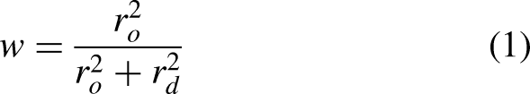
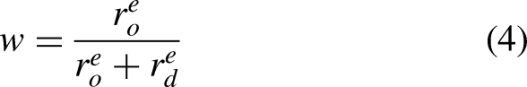
Equation (1) is the formula used for the Pythagorean expectation. Because this method uses a single exponent in calculating the winning percentage, models in the results section based on this formulation are referred to as single exponent models.
Pythagorean expectation alternatives
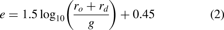
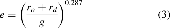
While the Pythagorean expectation formula provides reasonable estimates, improvements have been suggested to show better performance. Other approaches have adjusted the exponential from the integer value of 2 to 1.83 to fit the data better. Rather than using a static exponent for all teams, formulas that use a different exponent for each team have been developed, such as equation (2) developed by Clay Davenport.
30
Because this method uses a logarithm in calculating the exponential for each data point, models in the results section based on this formulation are referred to as logarithm models.
Model creation and metrics
A concern with using regression to fit coefficients is the potential of overfitting the data. 32 Although the concept was initially used in baseball, the idea has been expanded to other sports, 33 with adjustments made to the exponents to fit the available data. In the results section, we will apply a sample of the previously defined exponents from baseball and use nonlinear regression to fit a single exponent. Multiple folds of the data were used in this study to validate the calculated coefficients. The dataset was split into five random groups; four groups were used to train the model, and the fifth group was used to test the model’s performance. Five instances of each test correspond to each of the five random groups being excluded from the training data and used for the testing data. These same five groups were used for all presented results.
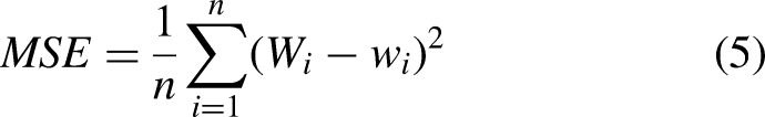
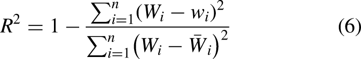
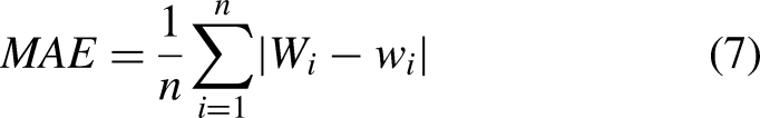
Three different metrics are used to evaluate empirically derived values: the mean squared error (MSE), the coefficient of determination (
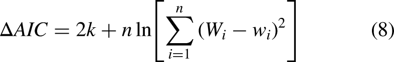
In addition, the Akaike information criterion (AIC)
34
is included for some of the models. Equation (8) is used to calculate the AIC
Raw statistics versus rates
While the total score-based methods have provided good results for other sports and are somewhat reasonable for the IPL, further investigation demonstrated that different team performance measures are better suited for the IPL. Our results indicate that rates are better than raw totals for the IPL. In particular, wickets also have a significant impact on the winning percentage. There is a continual alternation between offense and defense in most other sports. As mentioned above, an IPL match involves a single switch between the offensive and defensive teams.
It is not uncommon for a team to only score one more run than its opposition, but this is problematic for the Pythagorean methods based on run differential. The results are skewed when a team that bats second only wins by one (or few runs) but has a significant number of overs remaining. Net run rate (NRR) in equation (9) is a common statistic used in cricket to account for this discrepancy and uses the economies rather than the total number of runs; the ratio of runs to overs is also known as the economy
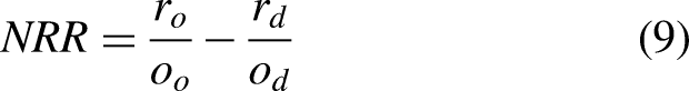
The use of economy rather than the total number of runs illustrates that the differences in the sport require a different approach to calculating the expected winning percentage than in other sports. Therefore, the desire was to investigate whether other team statistics might better estimate the winning percentage of an IPL team because of the different construction of the play of a match.
Algorithms
Two different methods were used to investigate other potential calculations of the winning percentage. The LASSO 32 and stepwise regression 32 were used to find models to fit the data. Over 40 different variables were considered for the model. The Appendix includes all considered variables.
Because both techniques have the potential to overfit models, all ten produced models were analyzed to determine commonalities. There are five datasets and two algorithms. Therefore, ten models are produced, with the first five models created with LASSO and each of the five datasets and the second five models created with stepwise regression and the five datasets. Each of the 10 models has, potentially, different independent variables that they use to calculate the expected winning percentage. Independent variables that appear in a vast majority of the 10 models are likely to influence the winning percentage. Independent variables that appear in only a few models are more likely a product of overfitting.
LASSO includes a regularization parameter 35 ; rather than selecting a single parameter, 100 were applied. Of the 100 resulting models, the model that produced the best mean squared error while not requiring more than seven decision variables were chosen for the LASSO results. The choice of a maximum of seven decision variables was made empirically as a tradeoff between accuracy and overfitting. LASSO was selected over ridge regression because it can force coefficients to be 0.
For the stepwise regression results, the maximum p-value for entry into the model was 0.05, and the minimum p-value for removal was 0.1. Interaction terms were not included in the stepwise analysis.
Results and discussion
Data from the 2008 through 2019 seasons were used for this analysis. Each data point includes the winning percentage and accumulated statistics during non-playoff matches for a team over an entire season; in most instances, the winning percentage and other statistics are for the 14 matches a particular team played. There were 100 data points, and all 100 data points were used in the analysis. Each test group consisted of 20 randomly selected data points, and the remaining 80 data points were used for model training. Each of the five test datasets contained unique data, so each of the 100 data points was a member of one and only one test dataset.
Traditional baseball coefficients
Table 1 compares results using standard coefficients from baseball as described in the previous section. From the two results, the best mean squared error is 0.0172, which is a difference in the winning percentage of 0.13. As a result, for the typical 14-match season, the expected error in the predicted number of wins is about 1.8. While the results are not terrible, improvement is still possible.
Baseball Pythagorean coefficients.
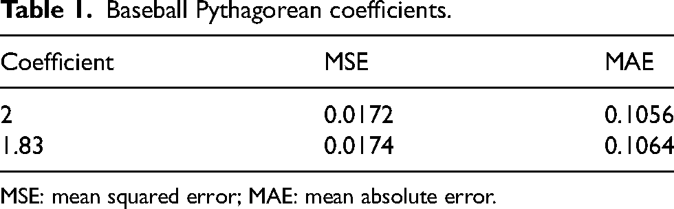
MSE: mean squared error; MAE: mean absolute error.
Fitting coefficients
Table 2 provides those results. Of note are the results from groups 1 and 2. While these two groups had the lowest MSE of the five groups for the testing data, these two MSE testing data values are lower than all training data MSEs; the two groups also have the highest training data MSE values. Investigating the MSE over all 100 data points for all five calculated exponents shows that the results are not very sensitive to the calculated exponent within the range of values in the table. As a first method to improve the results, nonlinear regression was used with cross-validation to determine the appropriate coefficient empirically.
Fit single exponent.
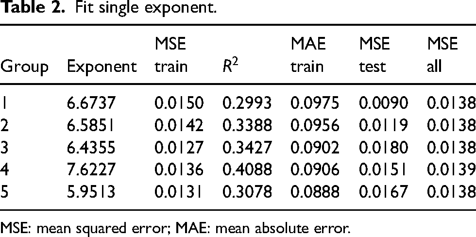
MSE: mean squared error; MAE: mean absolute error.
The average of the five exponents is approximately 6.65. As the next step of the investigation, exponents of 6.6 through 6.7 in steps of 0.01 were evaluated. For all 11 values of the exponent, the MSE agrees to six decimal places. However, 6.65 is the local minimum of the set. Suppose a single exponent is to be used. In that case, 6.65 is the recommended choice because it is the average of the five different training sets and the local minimum of evenly-spaced tested exponents. Due to the low sensitivity of the MSE over all 100 data points, any value between 6 and 7 would produce similar results.
While using the derived exponent is an improvement, the
Logarithmic exponent.
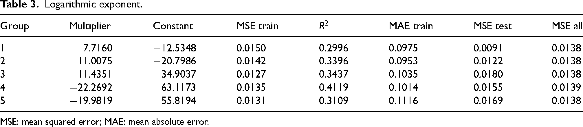
MSE: mean squared error; MAE: mean absolute error.
Power exponent.
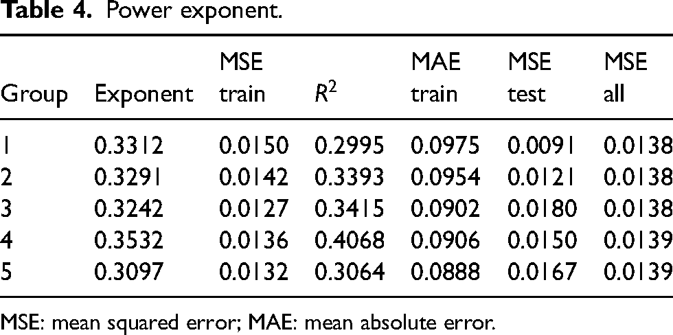
MSE: mean squared error; MAE: mean absolute error.
AIC values.
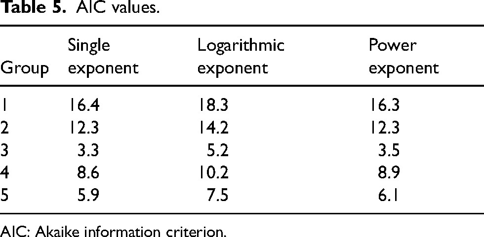
AIC: Akaike information criterion.
Rates rather than totals
As mentioned previously, for the IPL, the total number of runs scored and conceded is not as informative as using the economies that consider the total number of runs and the rate at which those runs were scored. For brevity, rather than repeating the results with the baseball coefficients, we will proceed to fit a single coefficient using equation (10)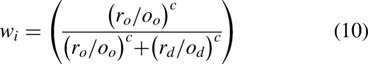
Single exponent for economies.
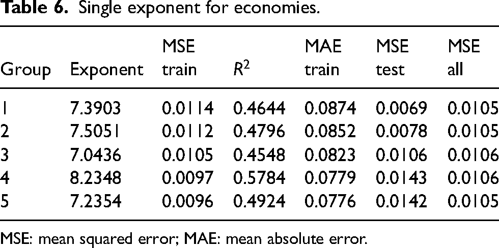
MSE: mean squared error; MAE: mean absolute error.
Comparing Tables 2 and 6, it can be seen that using economies rather than the total number of runs results in an improved value of both MSE,
Our results show that the IPL differs from other leagues because economies are more predictive of winning percentages than total runs. While using economies rather than total runs has produced a superior model, the expected error of approximately 1.4 wins per 14-match season could still be improved. Still, there is the question of whether other statistics could potentially provide superior results.
Independent variable selection
LASSO was applied to the five training datasets with the chosen solution with the minimum MSE while not having more than seven variables. There were over 40 variables under consideration. However, all non-rate variables were converted to a per-over basis based on the results above, indicating that over rates will likely be more effective than raw totals. The number 7 was chosen empirically. Table 7 has the numerical results, and Table 8 has the LASSO-identified variables; all variables are on a per-over basis.
LASSO result metrics.
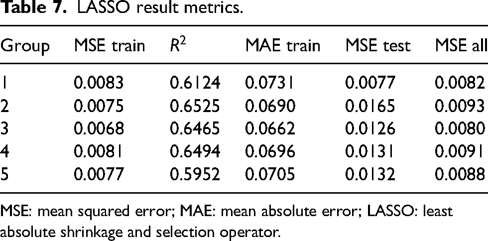
MSE: mean squared error; MAE: mean absolute error; LASSO: least absolute shrinkage and selection operator.
LASSO variables included.
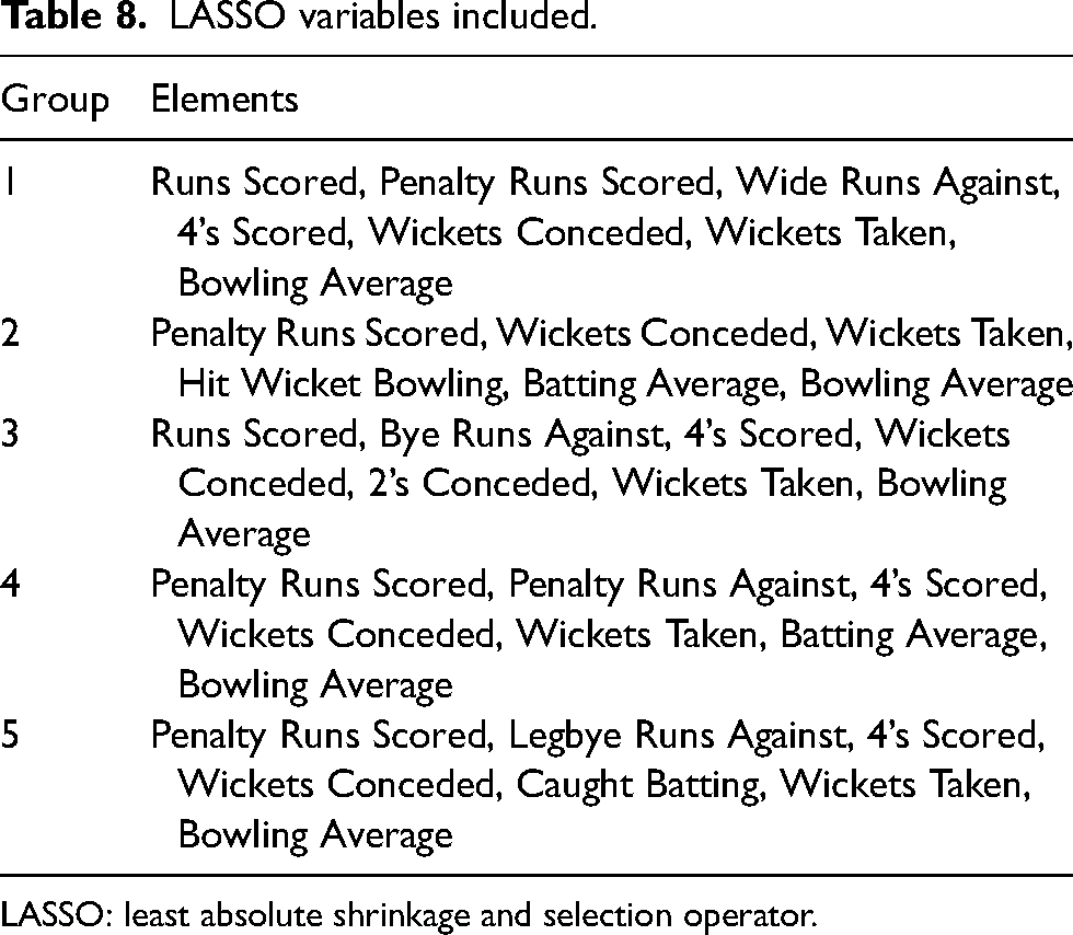
LASSO: least absolute shrinkage and selection operator.
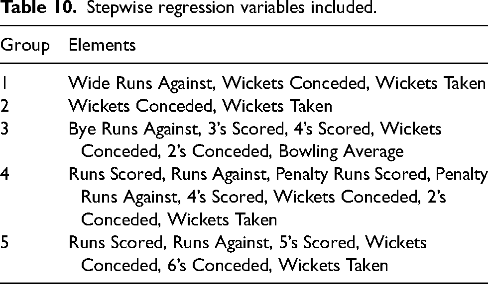
The five folds of data are to prevent overfitting the data. However, the variables included in the model are significantly different for all five test cases. Since all five groups are a random subsample of the population, the fact that the variables are different points to the potential of overfitting the data using a single model. As an alternative approach, stepwise regression was implemented to identify appropriate models. The numerical results are in Table 9 and Table 10 list the included variables for each model; all variables are on a per-over basis.
Stepwise regression metrics.
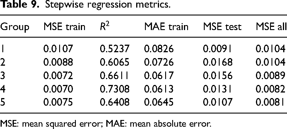
MSE: mean squared error; MAE: mean absolute error.
Stepwise regression variables included.
Final model construction
Comparing Tables 6, 7 and 9, it can be seen that the results for all methods are reasonably comparable, with each technique performing best (or tied for best) on at least one of the test datasets. Examining Tables 8 and 10, it can be noted that the only variables presented in at least nine of the 10 models are wickets taken and wickets conceded. Notably, these are the only two variables in the stepwise regression model for the second dataset. As mentioned previously, these values are based on a per-over rate. Regression was used to fit a linear model of only these two variables and an intercept term. Table 11 includes these results. It was known that the
Wickets only results.
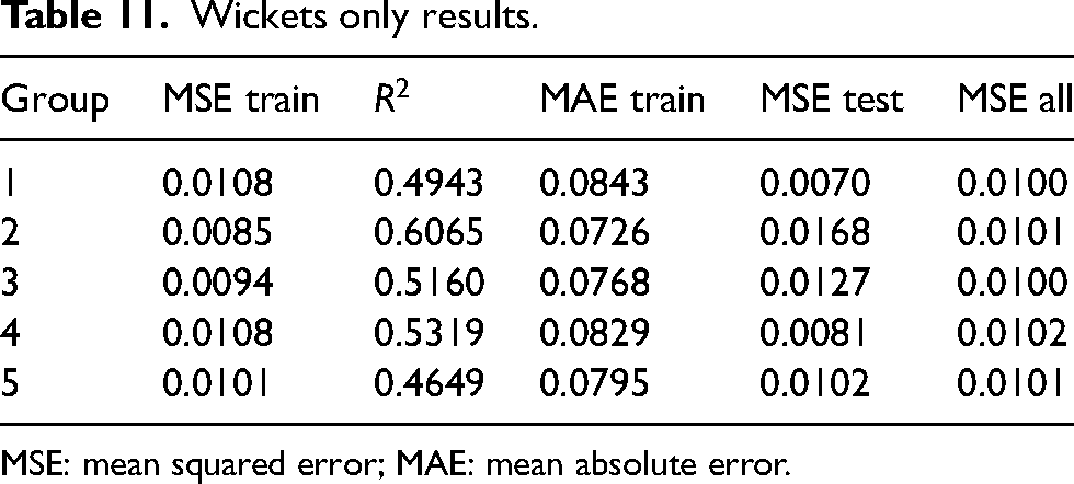
MSE: mean squared error; MAE: mean absolute error.
The Pythagorean solution for the economies reasonably predicts winning percentages, and the linear combination of wicket rates also predicts winning percentages. The five training datasets were individually used to fit equation (11).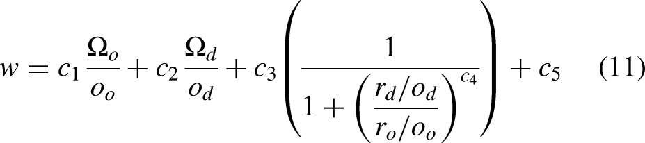
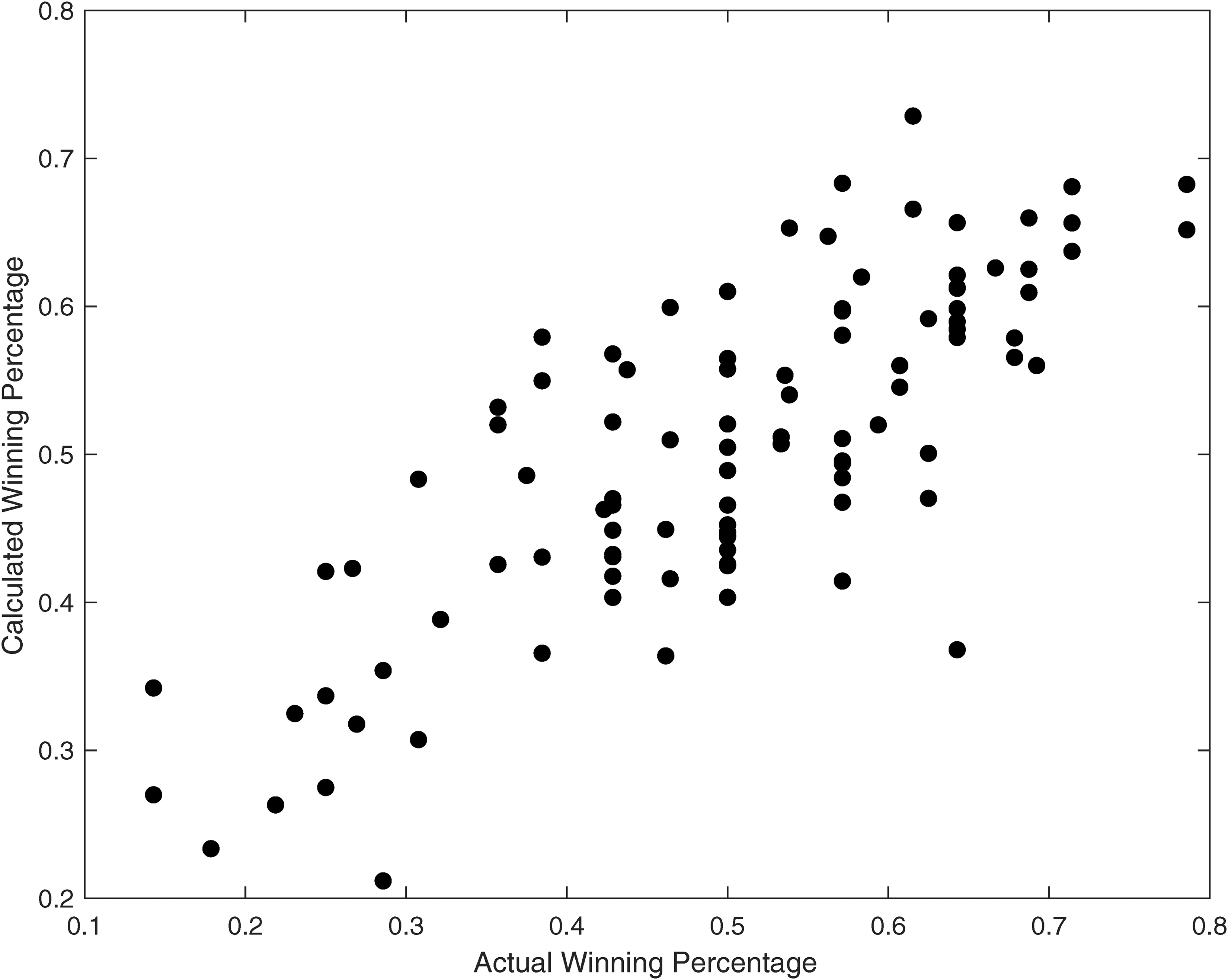
Calculated versus actual winning percentages.
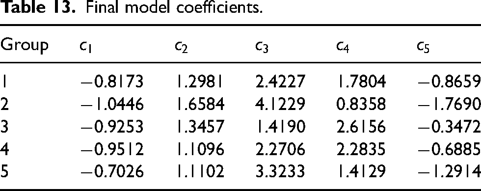
Combination of wicket rates and economies.
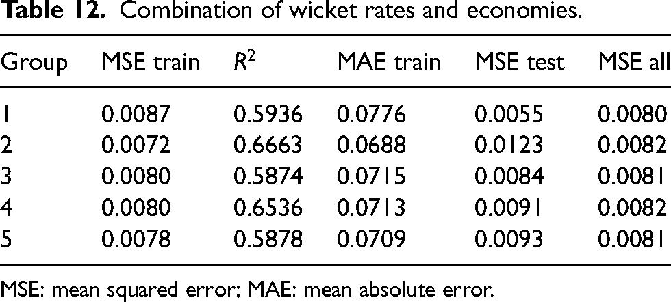
MSE: mean squared error; MAE: mean absolute error.
Final model coefficients.
The outliers in Figure 1 illustrate the value of calculating the expected winning percentage. As one example, consider the point in the lower right of the figure with a winning percentage of 64% (9 wins), but the underlying statistics estimated a winning percentage of 37% (5.2 wins). The team was fortunate and had a good season, and there was a desire to replicate the same level of success the following year. However, luck is usually not consistent in sports from one season to the next. 33 In comparison, consider the team in the upper right of the figure. The team had a winning percentage of 57% (8 wins) and an expected winning percentage of 68% (9.6 wins). While this second example is not as extreme as the first, it is a team that had a great year statistically but not as good of a year in terms of overall record. The team will likely perform better in the following season without significant changes as their luck regressed to the mean.
Logically, the wicket rate on offense would have a negative slope since fewer wickets fallen while batting tends to lead to higher scores and, thus, a better chance to win. Similarly, the positive slope for the bowling wicket rate follows the same logic. The fact that the exponent (
Conclusions
In many sports, the Pythagorean expectation approach provides reasonable estimates of the winning percentage of teams. For the IPL, the Pythagorean expectation approach offers reasonably accurate estimates but can use some improvement. Data from 12 seasons of the IPL was used along with nonlinear regression to find the exponent for the Pythagorean expectation approach that best predicted the winning percentage.
The results presented in this paper shows mathematically that the results improve with economies rather than total runs. Because of the unique nature of the IPL compared to other sports, rather than investigating the total number of runs, the economies were used to determine the expected winning percentages. This approach provided more accurate estimates for the training data and, more importantly, the testing data. However, NRR, as a typical team performance metric, implies this conclusion.
A follow-up question was whether statistics, in addition to or replacement of economy, might be a reasonable means of determining the expected winning percentage. To have an unbiased approach to considering alternative variables, both LASSO and stepwise regression fit models for the various training datasets. The ten models built by these two approaches over the five datasets included wicket rates, and most included additional variables. Linear regression fit models with only wicket rates as inputs. The results compared well with the Pythagorean economy model and the models with other variables determined by LASSO and stepwise regression.
The approaches of both a Pythagorean-based economy model and a linear wickets rate model had been determined to reasonably predict winning percentages. The final question was whether combining these two approaches would provide superior results. The combined model does perform better than either of the individual models.
The number of seasons for the IPL is significantly less than the number of seasons in the history of other major sports leagues such as Major League Baseball (MLB), the National Basketball Association (NBA), the National Hockey League (NHL), etc. and there are fewer teams in the IPL than these other leagues. As a result of these factors, there are fewer data points for the regression models. As additional data becomes available, the accuracy of these models may potentially improve. However, three different approaches were applied to determine models that reasonably predict a team’s winning percentage in the IPL. In all instances, rates needed to be considered rather than totals due to the unique structure of cricket. While the combination of the two base models has the best performance measures, the simpler base models have the advantage of having fewer variables and providing reasonably accurate results.
There is value in understanding whether a team has been lucky, unlucky, or is performing as expected. The results presented here help explain the amount of a team’s record in the IPL due to luck and the amount due to the underlying statistics. Knowing the expected win rate of a team will enable a better decision-making process for the team. In addition, understanding the impact of variables such as wickets and runs on overall winning percentages can help determine how management should construct a team. In addition, by using the expected winning percentage throughout the season, fans and club officials will be able not to panic as much if their team is not winning (but should be winning) and can temper their excitement if their team has been winning a lot, but has simply been very lucky.
Footnotes
Acknowledgements
I want to thank Vamsi Penumatsa for his initial concept that led to this work.
Declaration of conflicting interests
The authors declared no potential conflicts of interest with respect to the research, authorship, and/or publication of this article.
Funding
The authors received no financial support for the research, authorship and/or publication of this article.
Appendix – Considered Team Statistics
Runs Scored Runs Against Wide Runs Scored Bye Runs Scored Legbye Runs Scored Noball Runs Scored Penalty Runs Scored Wide Runs Against Bye Runs Against Legbye Runs Against Noball Runs Against Penalty Runs Against 1 Scored 2 Scored 3 Scored 4 Scored 5 Scored 6 Scored Wickets Conceded Caught Batting Bowled Out Batting Runout Batting LBW Batting C&B Batting Stumped Batting Hit Wicket Batting Obstruction Batting 1 Conceded 2 Conceded 3 Conceded 4 Conceded 5 Conceded 6 Conceded Wickets Taken Caught Bowling Bowled Out Bowling Runout Bowling LBW Bowling C&B Bowling Stumped Bowling Hit Wicket Bowling Obstruction Bowling Dot Balls Batting Dot Balls Bowling Average Batting Average Bowling