Sage Journals: Discover world-class research

Abstract

The prediction of future events and the preparation of appropriate behavioural reactions rely on an accurate perception of temporal regularities. In dynamic environments, temporal regularities are subject to slow and sudden changes, and adaptation to these changes is an important requirement for efficient behaviour. Bayesian models have proven a useful tool to understand the processing of temporal regularities in humans; yet an open question pertains to the degree of flexibility of the prior that is required for optimal modelling of behaviour. Here we directly compare dynamic models (with continuously changing prior expectations) and static models (a stable prior for each experimental session) with their ability to describe regression effects in interval timing. Our results show that dynamic Bayesian models are superior when describing the responses to slow, continuous environmental changes, whereas static models are more suitable to describe responses to sudden changes. In time perception research, these results will be informative for the choice of adequate computational models and enhance our understanding of the neuronal computations underlying human timing behaviour.

Keywords

Temporal context rapid recalibration timing time perception Bayesian models duration

Humans are remarkably sensitive to temporal regularities in their environment (Damsma et al., 2021; Di Luca & Rhodes, 2016; Jazayeri & Shadlen, 2010, 2015; Maaß et al., 2022; Narain et al., 2018; Rhodes, 2018; Rhodes & Di Luca, 2016; Rhodes et al., 2018; Tanaka & Yotsumoto, 2017). The detection and processing of such regularities is crucial for the prediction of future events and enables adjustments of behavioural responses. In dynamic environments, temporal regularities are often subject to slow as well as sudden changes, and an ongoing adaptation to these changes imposes a critical challenge for the human sensory system (Cicchini et al., 2012, 2014; Di Luca & Rhodes, 2016; Li et al., 2016; Petzschner et al., 2015, 2012; Rhodes, 2018; Rhodes & Di Luca, 2016; Riemer et al., 2016).

Several studies have shown that perceptual uncertainty about environmental aspects affect behaviour (Beierholm et al., 2009; Ernst, 2006; Kersten & Yuille, 2003; Knill & Richards, 1996; Körding & Wolpert, 2004, 2006; Lee & Wagenmakers, 2009; Ma et al., 2006; Maloney & Mamassian, 2009; Mamassian et al., 2002; Miyazaki et al., 2006; Moreno-Bote et al., 2011; Petzschner et al., 2015; Riemer et al., 2016; Sato & Aihara, 2011; Shi et al., 2013; Vilares & Körding, 2011; Vincent, 2015; Wei & Stocker, 2015). The Bayesian framework provides a simple and elegant way of formalising and describing human and animal behaviour in experimental tasks that require perceptual judgements under varying degrees of uncertainty. The applicability of the Bayesian framework has been demonstrated in various areas, such as visual detection of stimulus properties (Peelen & Kastner, 2014), control of goal-oriented movements (Elliott et al., 2014; Körding & Wolpert, 2004, 2006; Wolpert & Ghahramani, 2000; Wolpert et al., 1995), and temporal cognition (Cicchini et al., 2014; Di Luca & Rhodes, 2016; Maaß et al., 2019; Petzschner et al., 2012, 2015; Rhodes & Di Luca, 2016; Riemer et al., 2016; Sato & Aihara, 2011).

In the terminology of the Bayesian framework, humans combine previously acquired knowledge about, for example, temporal intervals (prior), with current sensory information (likelihood) to form a percept (posterior). This process is assumed to converge towards an optimal performance for a specific task (Ernst & Banks, 2002; Ernst & Di Luca, 2011; Hartcher-O’Brien et al., 2014; Hillis et al., 2002; Knill & Richards, 1996; Lee & Wagenmakers, 2009; Mamassian et al., 2002; Rhodes, 2018). Such a way of thinking and modelling phenomena is consistent with the free-energy principle (Friston, 2005, 2008; Friston et al., 2006; Friston & Stephan, 2007), where the brain seeks to reduce uncertainty to optimise behaviour through perception (Friston et al., 2017; Friston & Kiebel, 2009). In this sense, minimising free energy is, in terms of the Bayesian framework (i.e., model inference through priors, likelihoods and posteriors), analogous to optimising performance (Bogacz, 2017; Buckley et al., 2017; Ernst & Banks, 2002; Ernst & Di Luca, 2011; Friston, 2009, 2010; Friston et al., 2006; Friston & Kiebel, 2009; Friston & Stephan, 2007; Hartcher-O’Brien et al., 2014; Hillis et al., 2002; Parise & Ernst, 2016; Rohde et al., 2015).

Duration judgements are influenced by recent experiences (Damsma et al., 2021; Di Luca & Rhodes, 2016; Gu et al., 2016; Jazayeri & Shadlen, 2010, 2015; Maaß et al., 2022; Rhodes & Di Luca, 2016; Rhodes et al., 2018; Shi & Burr, 2016; Shi et al., 2013), both over long periods of time (Jazayeri & Shadlen, 2010, 2015; Roach et al., 2016), and in rapid contextual calibration (Di Luca & Rhodes, 2016; Rhodes & Di Luca, 2016; Rhodes et al., 2018). In this way, the perception of duration adheres to the principles of Bayesian inference, that is, it is the result of both memory traces about what has been previously experienced (temporal context) and a representation of a currently perceived duration (Cicchini et al., 2012; Di Luca & Rhodes, 2016; Jazayeri & Shadlen, 2010, 2015; Maaß et al., 2019; Rhodes, 2018). In their seminal work, Jazayeri and Shadlen (2010) presented subjects with a duration that had to be reproduced. In an experimental session, subjects were presented with a predetermined distribution of intervals that were sampled from a uniform-random distribution. The subjects’ responses were in accordance with Bayesian principles (and other models incorporating an influence of past trials): Relatively short intervals were over-reproduced, while relatively long intervals were under-reproduced, that is, their behaviour was biased towards the mean of a uniform sampling distribution. This phenomenon is known as Vierordt’s Law and has been reported in many other studies (Lejeune & Wearden, 2009; Riemer & Wolbers, 2020).

Extending these ideas, we recently posited a computational model of the dynamic updating of expectations within a single sequence of stimuli (Di Luca & Rhodes, 2016; Rhodes, 2018; Rhodes & Di Luca, 2016; Rhodes et al., 2018), and proposed that such a mechanism acts in parallel with a causal inference layer (Elliott et al., 2014; Kayser & Shams, 2015; Mendonça et al., 2016; Rhodes et al., 2018; Shams & Beierholm, 2010) that assigns priors given the relative evidence for their relation to previous instances. According to these dynamic models, priors are updated over time, trial-by-trial, stimulus-by-stimulus, which puts them in contrast to “static” Bayesian models of duration perception (Jazayeri & Shadlen, 2010, 2015; Roach et al., 2016; Shi et al., 2013). These latter accounts posit a single generalised prior that is known from the first trial of the experiment, and that is parameterised by the objective distribution of intervals presented in one complete session.

In a previous investigation, we presented subjects with a series of four isochronous tones, where the final tone was either earlier, on-time or later than expected (Di Luca & Rhodes, 2016; Rhodes & Di Luca, 2016). We found that the timing of the final tone after a regularly paced sequence was perceptually distorted: Stimuli presented earlier than expected were reported as slightly delayed, whereas stimuli occurring later than expected were reported as slightly earlier. This result suggests that the brain regularises deviant stimuli in accordance with expectations, that is, in line with Bayesian principles (Bayes, 1763; Freestone & Church, 2016; Gu et al., 2016; Hollingworth, 1910; Jazayeri & Shadlen, 2010, 2015; Knill & Richards, 1996; Lee & Wagenmakers, 2009; Shi et al., 2013).

In another study, we used the same task, but presented subjects with sequences of auditory stimuli that had on average shorter inter-stimulus intervals, and sequences of visual stimuli with on average longer inter-stimulus intervals (Rhodes et al., 2018). We found that subjects appear to update multiple duration priors contingent on the sensory modality, that is, a dynamic updating of expectations for separate, categorical priors.

In previous work, a simple Kalman filter (Cicchini et al., 2014; Di Luca & Rhodes, 2016; Petzschner et al., 2012; Rhodes et al., 2018) (Figure 1) was able to adequately describe subjects’ responses to dynamic changes in the environment. A Kalman filter is a system that alternates between two states: (1) priors about the duration of an event are combined with likelihoods using Bayesian principles leading to a posterior probability about the state of the world and (2) the resulting posterior becomes the prior for the next iteration of the model. Put simply, a Kalman filter is an iterative (dynamic) Bayesian model.

Figure 1.

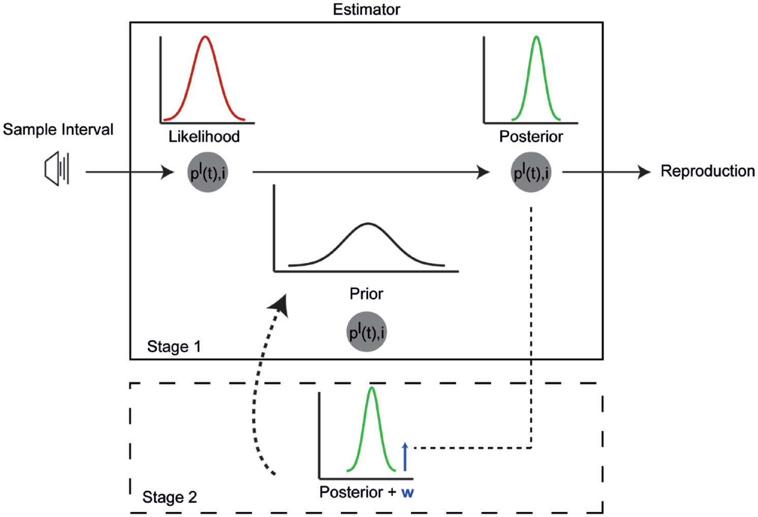
Illustration of a Bayesian (Kalman filter) account of subjective time in an isochronous sequence of six stimuli. In Stage 1, the sample interval is estimated by an internal Bayesian estimator as a measurement likelihood $p^{l} (t), i$ on a linear scale. The posterior estimate of the sample interval is determined by the combination of the likelihood and an a priori estimate of the interval $p^{l} (t), i$ . Stage 2, an added constant, is combined with the resultant posterior to balance complete fusion of the prior and likelihood in the following ith trial (Di Luca & Rhodes, 2016).

In the present study, we asked whether duration processing systems act in accordance with strict Bayesian “laws,” that is, whether posterior estimates for duration update in a way that is similar to a Kalman filter. In previous studies (Gu et al., 2016; Jazayeri & Shadlen, 2010, 2015; Jong et al., 2021; Rhodes et al., 2018; Roach et al., 2016; Shi et al., 2013), subjects were generally presented with time intervals sampled from uniform or Gaussian distributions of a specific range, and subsequently were asked to reproduce these intervals (by terminating a second interval once it has reached the same duration). The mean responses for each sampled interval are then computed and presented as a function of the physical interval presented (Gu et al., 2016; Jazayeri & Shadlen, 2010, 2015; Rhodes et al., 2018; Roach et al., 2016; Shi et al., 2013). Thus, what has been analysed in these experiments are summary metrics for each interval—which neglect the trial-by-trial estimates for each subject. However, these trial-by-trial effects can reveal important information about rapid updating of priors and temporal expectations, and ultimately about the adaption of the sensory system to sudden environmental changes. There are two distinct possibilities about rapid contextual updating of priors in interval timing: Gradual or sudden adaptation to environmental changes.

To highlight trial-by-trial metrics, we presented subjects not with a uniform random sample of intervals, but instead with a sequential sampling pattern that followed either a sinusoidal or square pattern (Figure 2b). We used the sine wave condition to test for adaptation to gradual changes and the square condition to test for adaptation to sudden changes in the environment. Subjects reproduced intervals using the classic ready-set-go procedure for interval timing to each sampling pattern (Jazayeri & Shadlen, 2010, 2015). Our results present clear evidence that the subjects’ behaviour follows Bayesian principles through rapid Bayesian updating. In addition, we compare our Kalman filter model to static models, and find that dynamic Bayesian models best describe the data.

Figure 2.

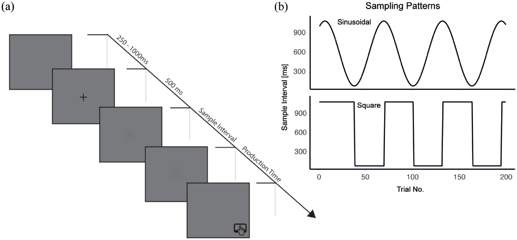
Methods. (a) The ready-set-go procedure. Subjects were presented with two Gaussian patches that determined the sample interval. Subjects were required to complete the sequence by pressing the spacebar (go!) when, after the set signal, the same time had elapsed as between the ready and set signal. (b) Sampling patterns for the sine wave and square wave conditions.

Methods

Participants

Seventeen undergraduate students from Nottingham Trent University took part in the experiment (M_age = 20.94, SD_age = 0.52, range: 18–26). All participants gave written informed consent. The School of Social Sciences Research Ethics Committee (SREC) approved this experiment and the methodology involved. Participants were naïve to the structure of the study (i.e., the interval sampling patterns) and all had normal or corrected-to-normal vision.

Stimuli

The experiment was performed in a quiet room. All stimuli were presented on a MacBook Screen, using PsychoPy3 (Peirce et al., 2019). During an experimental block, a 10 × 10 pix fixation cross was presented at the centre of the screen (Figure 2a). In each trial, a “ready” and “set” stimulus was presented, both consisting of a 128 × 128 pix diameter linear Gaussian Gabor patch, which appeared in the centre of the screen, and was identical for each trial in the experiment.

Procedure

All participants performed a ready-set-go reproduction task under two conditions: sine wave sampling and square wave sampling, that is, the standard durations were taken from a sample, the mean of which changed over trials (and hence over time) according to a sinusoidal versus a square function (Figure 2b). The square wave sampling condition consisted of two intervals of 100 and 1100 ms. In the sine wave condition, durations were calculated by taking the sine of a range of arbitrary intervals (in this case [1:31]), multiplying by 1000, adding 1200 to each value, and then dividing by 0.5. This gives the sine wave sampling distribution as presented in Figures 2b and 3a.

The presentation order of both conditions was counterbalanced across participants, and participants started each block at the same point (Trial Number 1). In each block, participants were presented with a sampling pattern of a total of 200 trials. Each trial started with a 500-ms fixation cross (Figure 2a). Subjects were presented with a “ready” signal (50 ms), followed by an inter-stimulus interval determined from the sampling patterns and ended with the “set” signal (50 ms). Participants were instructed to press the spacebar when they perceived that the duration between the “set” signal and their button press matched the length of the initial interval between the “ready” and “set” signals.

Results

As expected, participants adjusted their responses to the standard sampling intervals. Figure 3 shows that participants performed in accordance with Bayesian inference: Their responses follow the sampling patterns of each condition—but they do so in a way that conforms to a regression towards the mean. In other words, responses generally do not peak above the longest or lie below the shortest duration in each sampling pattern. To test whether participants were more accurate (i.e., reproduced durations as close as possible to the sample interval) in the square versus the sine wave condition, we calculated for each trial the absolute differences between the presented sample interval and the reproduced duration (i.e., the difference between the red and blue lines in Figure 3). A paired samples Bayesian t-test with a default Cauchy prior scaled to .707 confirmed that the evidence was in favour of there being a statistical difference between the conditions, such that the responses were more accurate in the sine wave sampling condition (Figure 4a and b; µ = 128.48, σ = 75.29) than in the square wave condition (µ = 212.10, σ = 95.04), BF₁₀ = 8.41^e+17.

Figure 3.

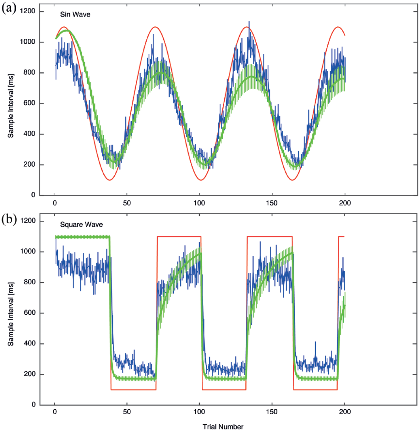
Results from the experiment. Subjects reproduced intervals sampled either from a sine wave or a square wave set (red lines). Blue lines show the subjects’ responses as a function of the interval presented (with standard error of mean across subjects). A Bayesian updating model (Kalman filter) provides a reasonable description to the sine wave and square wave sampling patterns (green lines).

Figure 4.

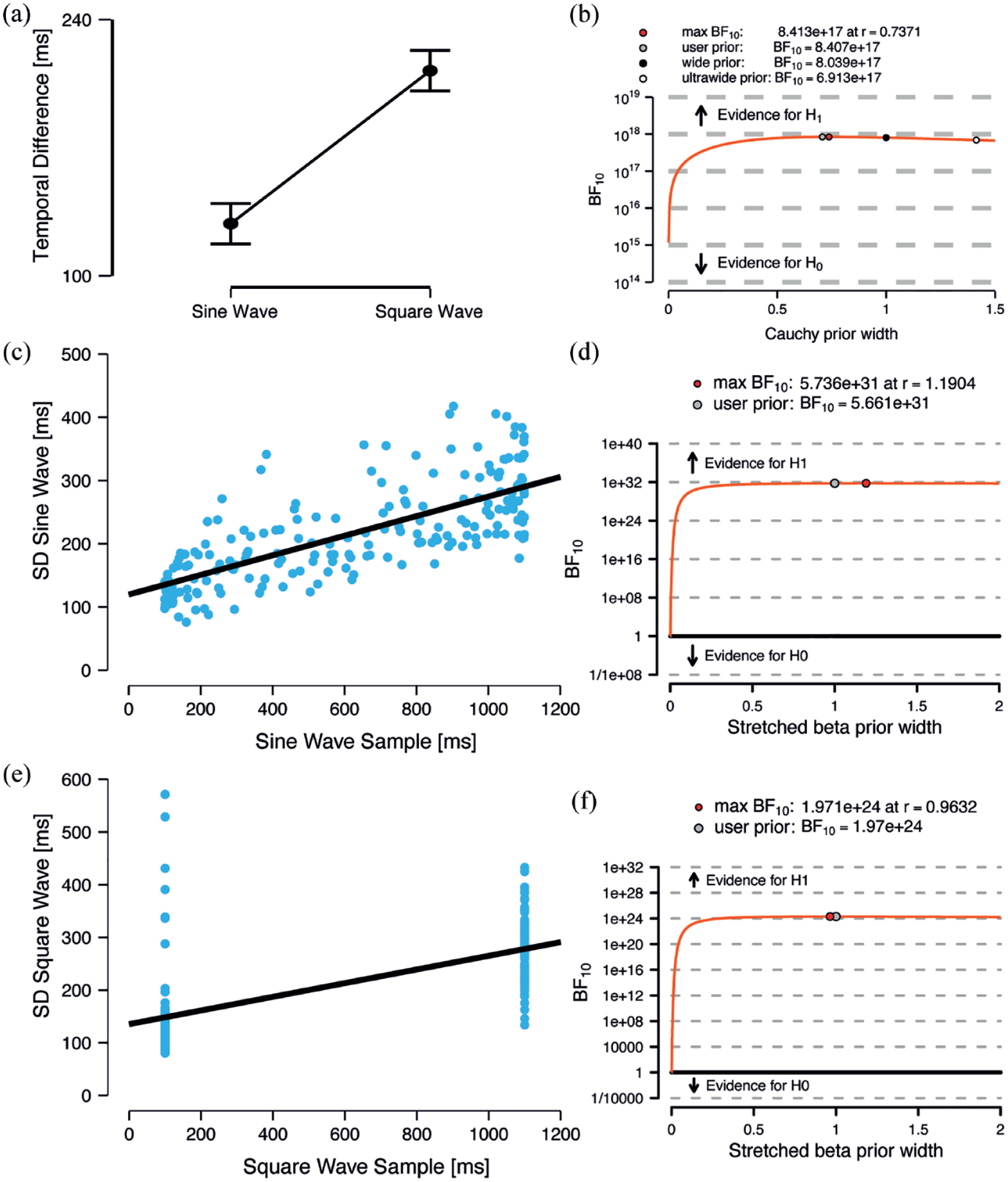
Results of the experiment. (a) The difference between the presented interval and the subjects’ responses for the sine wave and square wave sampling patterns. (b) Robustness check for the paired sample Bayesian t-test between both conditions. The Cauchy prior width plotted as function of the estimated Bayes Factor confirms a robust effect. (c) The standard deviation (across subjects) as a function of the presented interval for the sine wave sampling pattern and (e) for the square wave sampling pattern. (d) Robustness checks for the Bayesian paired correlations for the sine wave sampling pattern and (f) the square wave sampling pattern with the Bayes Factor plotted as a function of a stretched beta prior confirm a robust effect.

Allied to this, the standard deviation across subjects for each trial n increased (or decreased, respectively) with the magnitude of the tested sample, according to the Weber–Fechner law (Fechner, 1860; Gibbon, 1977; Gibbon et al., 1984) for perception. To test whether each sampling adhered to this law, we plotted the standard deviation of each sampling pattern for all trials as a function of the presented sample interval (Figure 4c and e). A Bayesian paired correlation test between the sample interval and the standard deviation over all trials revealed that they were correlated for both the sine wave (r = .73, BF₁₀ = 5.66^e+31) and the square wave condition (r = .67, BF₁₀ = 1.97^e+24) (Figure 4d and f), indicating adherence to the Weber–Fechner law.

Figure 3 also shows that the reproduction of relatively long intervals (i.e., 1100 ms in the square wave condition) were already biased towards lower values in the first trials, that is, when the relatively short intervals of that condition haven’t been presented yet. This is a consequence of both conditions being presented in a counterbalanced order, so that half of the participants have already experienced the complete range of intervals from the sine wave condition. For participants who performed the square wave condition first, this bias was significantly reduced (t₁₃ = 3.1, p = .004). However, even for those participants a residual bias towards lower values was still observable (mean reproduced interval in the first 38 trials was 1013 ms), which might be due to a general tendency to respond rather early than late in temporal reproduction tasks (Akdoğan & Balcı, 2017; Riemer et al., 2019).

Comparing static and dynamic models of perceived duration

In the following section, we test the key motivation of this work: can both static and dynamic interval timing models describe adequately regression effects in interval timing, and which of the following models best describes the data?

Dynamic Bayesian model

We have previously shown that the performance in interval timing tasks can be modelled with a Kalman filter (Di Luca & Rhodes, 2016; Jong et al., 2021; Rhodes, 2018; Rhodes & Di Luca, 2016; Rhodes et al., 2018). Accordingly, we used a Kalman filter to model the results of the present experiment. We modelled the “perceived” interval as the posterior distribution, that is, the integration of the current sensory evidence (likelihood) with a priori expectations about the stimulus’ duration (prior). In contrast to “static” Bayesian models (Jazayeri & Shadlen, 2010, 2015; Roach et al., 2016; Shi et al., 2013), we propose that these expectations are not static (Cicchini et al., 2014; Di Luca & Rhodes, 2016; Petzschner et al., 2012; Rhodes, 2018; Rhodes et al., 2018), but that they are iteratively updated by the incoming sensory evidence about duration. The likelihood probability distribution $p^{l} (t)$ is the probability of perceiving a specific duration l at time t. Gaussian distributions with a mean equal to the presented interval, and variance $σ^{2}$ describe the noise in the representation of intervals. Given the scalar property of time perception (Church et al., 1994; Gibbon, 1977; Gibbon et al., 1984), which states that the variance of a given estimate increases given the magnitude of the stimulus to be estimated, we calculated $σ^{2}$ as a power law

σ^{2} = M \cdot D^{b}

(1)

D is the intensity of the stimulus in physical units (in our case duration in ms), M is an exponent that depends on the stimulus, and b is a proportionality constant that depends on the units of measurement (D). We obtained the posterior probability distributions $p^{q} (t)$ by multiplying the probabilities of the likelihood $p^{l} (t)$ and the prior $p^{p} (t)$

p^{q} (t) \propto p^{l} (t) \cdot p^{p} (t)

(2)

We obtained the prior probability distribution $p^{p} (t)$ using the posterior probability $p^{q} (t)$ for the previous stimulus (i.e., $p^{p} (t)$ for the time t-IOI; inter-onset interval). The added constant ω leads to a prior with heavy tails (Di Luca & Rhodes, 2016; Roach et al., 2006) that allows sudden changes in duration magnitude, and then decreases the tendency of fully incorporating the posterior into a new prior (thus mitigating the increase in false alarms; Carnevale et al., 2015). This is expressed by

p^{p} (t + IOI) \propto p^{q} (t) + ω

(3)

Static model

In addition to the dynamic Bayesian model defined above, we realised a static model based on previous work—but with a twist. In these models, a single static prior distribution is constructed from an objective sampling distribution $p^{p} (t)$ , and combined with current sensory evidence about the perceived duration on a given trial $p^{l} (t)$ . The combination of the prior and posterior leads to the posterior distribution from which a sample is taken (maximum a posteriori estimate—the mode of the posterior) to model the reproduced duration. This leads to the same computation as equation (2); however, this model is static, and as such, there is no updating of the prior. The twist, to make the model more in unison with present work, is that we again fit the variance $σ^{2}$ of each sample duration with the power law as outlined in equation (1). In previous work, the $σ^{2}$ is specified as linearly increasing with the mean of the likelihood (Jazayeri & Shadlen, 2010). It is also important to note, that these static models do not consider any trial-by-trial data, and to facilitate with previous work, we plotted the actual sample interval on the x-axis, and the reproduced duration on the y-axis (Figure 4). We thus fit the model to this “summarised” representation of the data.

Model fitting and model comparison

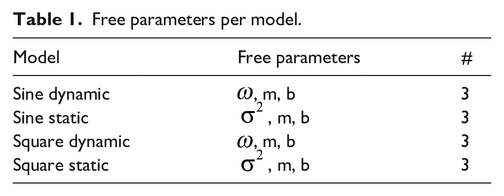
To obtain the model fits for both the square and sine wave trial sequences, we calculated the values (MAP) of the posterior probability distributions for the presented duration, for each of the models described above. The free parameters (see Table 1) were fit to the responses of each participant in all trials, by calculating the error between the model’s output (i.e., the mean of a model posterior distribution) and the actual reproduced duration. We used MATLABs fminsearch function to maximise the likelihood of model parameters for each subject—for each model (Table 1). We calculated the Akaike Information Criterion (AIC) as a metric of model evidence and interpreted these results using the rules of thumb given by Burnham and Anderson (2003).

Table 1.

Free parameters per model.

Model	Free parameters	#
Sine dynamic	$ω$ , m, b	3
Sine static	$σ^{2}$ , m, b	3
Square dynamic	$ω$ , m, b	3
Square static	$σ^{2}$ , m, b	3

Our model comparison (Figure 5e), using AIC, selected the dynamic Bayesian model as the preferred model for the sine wave sampling data (AIC = −16.42 ± 0.18), and the static model for the square wave data (AIC = −13.69 ± 0.14). In sum, the Kalman filter does a better job of describing the data than a static model in the sine sampling condition, that is, with gradual changes in the (temporal) environment. Second, the static model better described the square wave sampling condition; however, this is a trivial result, as the model is simply fitting a regression line between two points in the static model, whereas in the Kalman filter models, there are trial-by-trial updating of prior probabilities, which in turn leave more room for fitting error. That said, it is difficult to compare the two models, given the divergence in the number of conditions across models, and how different they are in dynamics.

Figure 5.

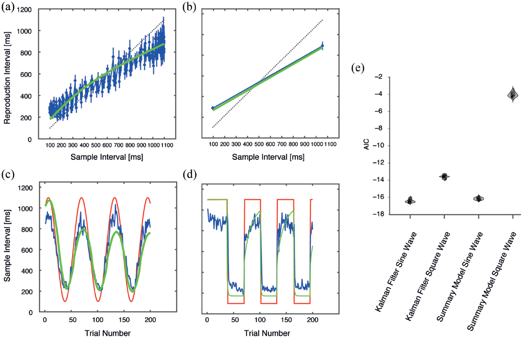
Results of the model fitting and model comparison. (a) Static model for the sine wave sampling condition, with reproduction interval as a function of the sample interval. In all graphs, blue lines indicate participant mean data, while green lines are the best fitting model output. (b) Static model for the square wave sampling condition. (c) Dynamic model for the sine wave condition, and (d) dynamic model for the square wave sampling condition. Red lines indicate the actual samples presented to participants. (e) AIC model comparison. Error bars denote standard error of the mean.

Discussion

In this work, we investigated human timing behaviour under conditions of gradual versus sudden changes of temporal contexts. Instead of focusing on static metrics on temporal context effects in interval timing, we instead focused on and compared trial-by-trial metrics.

We found that participants behave in a way that is predicted by Bayesian accounts of time perception (Di Luca & Rhodes, 2016; Rhodes, 2018; Rhodes et al., 2018), that is, participants consider their recent sensory experiences to inform their responses. Participants did not meander away from the mean. Even in the first few trials of each sampling pattern, there are no apparent anti-Bayesian responses. Subjects’ duration estimates do not fall outside the range of sampled values that were presented, but rather they appear to track the sampling patterns and regress towards the mean. This finding is important, as one criticism of work into temporal context effects in interval timing is that because they are modelled “in static,” that is, they assume a fixed objective prior based solely on the sampling distribution, it is difficult to believe that subjects know what the objective prior is within a few trials of starting the experiment. Our data demonstrate that subjects are reacting to dynamic temporal changes in recent sensory experiences in a “lawful” way.

The data continued to act in what appears a lawful way by adhering to the Weber–Fechner law for perception (or oftentimes called the “Scalar Property” in the field of interval timing; Church et al., 1994; Gibbon et al., 1984). We found that as the sample presented to subjects increased in duration, so did the sample standard deviation. This finding, that there is more variance across subjects in longer sampling intervals (and vice versa), serves as a sanity check that subjects are behaving in a predictable way with regards to interval estimates.

The first question we asked in this article was whether participants behave in a way predicted by Bayesian accounts of interval timing at the trial-by-trial level. The second question was whether static (Jazayeri & Shadlen, 2010, 2015; Rhodes, 2018; Shi et al., 2013) or dynamic Bayesian models do a better job of describing trial-by-trial interval sampling data. We found that a dynamic Bayesian model applied to interval timing can indeed approximate human behaviour in our task (Figures 3 and 4). This is important, as it adds credence to previous work that such models can be applied to “temporal-order” and “on-time” judgements in a rhythmic timing task (Di Luca & Rhodes, 2016; Rhodes, 2018; Rhodes & Di Luca, 2016; Rhodes et al., 2018). Our work expands upon these models by highlighting the trial-by-trial effects, rather than summary metrics—such as the mean. Bayesian updating models fit the data better than the static model for the sine wave condition (Figure 5), but there is not an incredible difference between the fit of the static model compared to the dynamic model. It is important to highlight here that the dynamic model is one (Bayesian) way to model trial-by-trial data (Figure 3) in this instance (though others have recently worked on this too; Visalli et al., 2021). To facilitate model comparison, we ignored any trial-by-trial dynamics in our data, and instead calculated mean values as a function of the sample intervals presented across the experiment. In this way, we lose variability, data points and insight by summarising the data. This is not to say static models are unimportant, but more so to highlight limitations in their application.

In general, both models were a better fit to the sine wave sampling pattern (as opposed to the square wave sampling pattern). Considering the best overall model fits and subjects’ responses (cf. Figure 3), we can see that the model tracks the sine wave sampling pattern better than the square wave sampling pattern. We might speculate here that the “surprise” of suddenly changing (and as such, adaptation processes) from one value to another value at the other end of a scale, might be driving such a difference in fit, and the difference in tracking. This is not entirely surprising, as Bayesian “surprise” is a concept that is firmly integrated within the free-energy principle of perception and action (Friston, 2005, 2008, 2010; Friston et al., 2006, 2017; Friston & Kiebel, 2009; Friston & Stephan, 2007).

Developed from the predictive coding model of perception (Friston & Kiebel, 2009; Hosoya et al., 2005; Huang & Rao, 2011; Kilner et al., 2007; Rao & Ballard, 1999; Sedley et al., 2016; Shi & Burr, 2016; Spratling, 2010; Srinivasan et al., 1982; Vuust et al., 2009; Vuust & Witek, 2014), the free-energy principle was influenced by Helmholtz’ ideas of “perception as unconscious inference” and statistical thermodynamics (Helmholtz, 1866), and the relatively new concept of machine learning (Buckley et al., 2017; Clark, 2013). This idea, that perceptions are the result of the probabilistic modelling of their causes, has seen a rise in prominence of “Bayesian Brain” and “Predictive Coding” accounts of brain function. Given this, the free-energy principle, and as such, predictive processing, is analogous to a simple Kalman filter (Friston et al., 2017; Kneissler et al., 2015), the model that we present here.

After the slight detour through defining the free-energy principle, Bayesian “surprise” is the difference between an internal (a prior) model of the world and current sensory information (the likelihood function). We could posit therefore, that our data might be explained by the (relatively) large difference (and change) from one value to another in the square wave sampling pattern, inciting a large prediction error, and as such, a large amount of “surprise.” The magnitude of this surprise culminates in a large difference between what is expected—and what is perceived, which manifests in a slower updating of the prior.

Limitations and outlook

In this study, our aim was to investigate the impact of rapid or incremental changes in temporal context on interval perception. One problem consists in the implementation of very short intervals (100 ms) to mark the lower bound of tested intervals. This interval lengths lies below the threshold for minimal reaction time in simple reaction time tasks (Woods et al., 2015). Although, except for the sudden steps in the square wave condition, our experimental design allowed for a certain degree of anticipation of the interval between the “ready” and “set” stimulus (a 100-ms interval did occur either in a sequence of equal intervals or in a sequence of slowly and continuously decreasing intervals. As such, participants’ responses were, in all probability, influenced by minimal reaction times, and as such reduced the sensitivity of our paradigm.

A further consideration for this work is in how Bayesian updating models fit into the flexibility–stability paradox. The flexibility–stability paradox raises the question of how short-term contextual changes require rapid updating of the prior (at the expense of stability), while simultaneously modelling a prior that is resistant to recent experience (at the expense of flexibility). Recent research and modelling has explored non-Bayesian explanations for this paradox (Killeen & Grondin, 2022; Salet et al., 2022; Taatgen & van Rijn, 2011), which further highlights the need to address this paradox within a Bayesian framework. One potential approach to address this challenge is the integration of hierarchical priors (Rhodes et al., 2018) and a causal inference layer that determines which priors should be updated (or not) based on the similarity or dissimilarity of incoming sensory information (Elliott et al., 2014; Salet et al., 2022; Taatgen & van Rijn, 2011). By incorporating these elements into Bayesian models, we may be able to better account for the flexibility–stability paradox and enhance our understanding of temporal perception through a Bayesian lens.

Alternative models

Time perception and its mechanisms have been extensively examined from various angles, each model bringing its own set of insights and assumptions. An essential element seen across models is the representation of perceived duration stored in some central memory framework (Bausenhart et al., 2014; Lejeune & Wearden, 2009; Salet et al., 2022; Shi & Burr, 2016; Taatgen & van Rijn, 2011; Wehrman et al., 2018). However, the methodology to arrive at this representation, and the consequential context effects, show a rich tapestry of approaches.

One of the models that stands at an interesting crossroads of this discussion is the formalised multiple trace theory of temporal preparation (fMTP). The unique associative learning mechanism in fMTP posits a relationship between time cells and a layer of readout neurons. When extended, this model shows that context effects, such as those observed in Vierordt’s law or sequential effects (as in the work presented here), emerge naturally. The fMTP’s framework is especially intriguing because it finds resonance with other models yet holds its distinction. For instance, both Bayesian observer models and sequential-updating models represent time through mathematical operations like Bayesian integration into prior distributions (Di Luca & Rhodes, 2016; Petzschner et al., 2012; Shi et al., 2013) or averaging durations with recency-weighted techniques (Taatgen & van Rijn, 2011). The Internal Reference Model and the mixed-pool model follow similar principles. What sets fMTP apart, however, is the neural embodiment of these principles. Durations are represented through distinct neural properties of the time cell layer, and the arising context effects stem from Hebbian learning dynamics between this layer and the readout circuit. This bridging of neural circuitry and time representation showcases the versatility and depth of the fMTP model (Salet et al., 2022).

Contrastingly, the mixed-pool model (Taatgen & van Rijn, 2011) underscores a blend of recent experiences shaping our perception of time. It suggests that representations of different time intervals can inadvertently influence each other, highlighting the significance of memory processes. The Internal Reference Model (Bausenhart et al., 2014), meanwhile, champions the dynamism in time perception, and emphasises the continual updating of an internal reference, especially in a sequential stimulus environment such as the one implemented in the present study.

Through the prism of a simple Kalman filter, our model illuminates the facets of dynamic Bayesian models in understanding perceived durations, especially in ever-changing (and sometimes sudden) temporal contexts. While our model contributes to this discourse by underscoring the probabilistic nuances in human timing behaviour, it is pivotal to understand its orientation within the larger tapestry of theories on temporal perception, and how similar models contribute to our understanding.

Conclusion

To summarise, we demonstrate that a simple Kalman filter (a dynamic Bayesian model) can adequately capture changes in perceived duration in a sequential sampling task with rapid and surprising changes in temporal context. We assert that static models, and as such, static temporal priors, could also model data with Kalman filters, to capture the fast and slow uptake of environmental information about time, and in doing so provide more insights into the neurocomputations underlying such processes. As such, models of time perception that adhere to such frameworks seem like a good bet when trying to understand how time might be processed in the brain.

Footnotes

Declaration of conflicting interests

The author(s) declared no potential conflicts of interest with respect to the research, authorship, and/or publication of this article.

Funding

The author(s) received no financial support for the research, authorship, and/or publication of this article.

ORCID iD

Darren Rhodes

Data accessibility statement

The raw data for this study are available on the Open Science Framework: , and any analysis or modelling scripts are available on request.

References

Akdoğan

Balcı

(2017). Are you early or late? Temporal error monitoring. Journal of Experimental Psychology: General, 146(3), 347–361. https://doi.org/10.1037/xge0000265

Bausenhart

K. M.

Dyjas

Ulrich

(2014). Temporal reproductions are influenced by an internal reference: Explaining the Vierordt effect. Acta Psychologica, 147(C), 60–67. https://doi.org/10.1016/j.actpsy.2013.06.011

Bayes

(1763). An essay towards solving a problem in the doctrine of chances. Philosophical Transactions of the Royal Society of London, 53, 370–418. https://doi.org/10.1098/rstl.1763.0053

Beierholm

U. R.

Quartz

S. R.

Shams

(2009). Bayesian priors are encoded independently from likelihoods in human multisensory perception. Journal of Vision, 9(5), 23–23. https://doi.org/10.1167/9.5.23

Bogacz

(2017). A tutorial on the free-energy framework for modelling perception and learning. Journal of Mathematical Psychology, 76, 198–211. https://doi.org/10.1016/j.jmp.2015.11.003

Buckley

C. L.

Kim

C. S.

McGregor

Seth

A. K.

(2017). The free energy principle for action and perception: A mathematical review. Journal of Mathematical Psychology, 81, 55–79. https://doi.org/10.1016/j.jmp.2017.09.004

Burnham

K. P.

Anderson

(2003). Model selection and multimodel inference: A practical information-theoretic approach. Springer.

Carnevale

Lafuente

de Romo

Barak

Parga

(2015). Dynamic control of response criterion in premotor cortex during perceptual detection under temporal uncertainty. Neuron, 86(4), 1067–1077. https://doi.org/10.1016/j.neuron.2015.04.014

Church

R. M.

Meck

W. H.

Gibbon

(1994). Application of scalar timing theory to individual trials. Journal of Experimental Psychology: Animal Behavior Processes, 20(2), 135–155.

10.

Cicchini

G. M.

Anobile

Burr

D. C.

(2014). Compressive mapping of number to space reflects dynamic encoding mechanisms, not static logarithmic transform. Proceedings of the National Academy of Sciences, 111(21), 7867–7872. https://doi.org/10.1073/pnas.1402785111

11.

Cicchini

G. M.

Arrighi

Cecchetti

Giusti

Burr

D. C.

(2012). Optimal encoding of interval timing in expert percussionists. Journal of Neuroscience, 32(3), 1056–1060. https://doi.org/10.1523/jneurosci.3411-11.2012

12.

Clark

(2013). Whatever next? Predictive brains, situated agents, and the future of cognitive science. Behavioral and Brain Sciences, 36(3), 181–204. https://doi.org/10.1017/s0140525x12000477

13.

Damsma

Schlichting

van Rijn

(2021). Temporal context actively shapes EEG signatures of time perception. The Journal of Neuroscience, 41(20), 4514–4523. https://doi.org/10.1523/jneurosci.0628-20.2021

14.

Di Luca

Rhodes

. (2016). Optimal perceived timing: Integrating sensory information with dynamically updated expectations. Scientific Reports, 6, Article 28563. https://doi.org/10.1038/srep28563

15.

Elliott

M. T.

Wing

A. M.

Welchman

A. E.

(2014). Moving in time: Bayesian causal inference explains movement coordination to auditory beats. Proceedings of the Royal Society B: Biological Sciences, 281(1786), 20140751–20140751. https://doi.org/10.1523/jneurosci.5561-10.2011

16.

Ernst

M. O.

(2006). A Bayesian view on multimodal cue integration. In Knoblich

Thornton

Grosejan

Shiffrar

(Eds.), Human body perception from the inside out (pp. 105–131). Oxford University Press.

17.

Ernst

M. O.

Banks

M. S.

(2002). Humans integrate visual and haptic information in a statistically optimal fashion. Nature, 415(6870), 429–433. https://doi.org/10.1038/415429a

18.

Ernst

M. O.

Di Luca

(2011). Multisensory perception: From integration to remapping. In Trommershauser

Körding

K. P.

M. S.

Landy

(Eds.), Sensory cue integration (pp. 224–250). Oxford University Press.

19.

Fechner

G. T.

(1860). Elemente der psychophysik. Breitkopf & Härtel.

20.

Freestone

D. M.

Church

R. M.

(2016). Optimal timing. Current Opinion in Behavioral Sciences, 8, 276–281. https://doi.org/10.1016/j.cobeha.2016.02.031

21.

Friston

(2005). A theory of cortical responses. Philosophical Transactions of the Royal Society B: Biological Sciences, 360(1456), 815–836. https://doi.org/10.1038/335311a0

22.

Friston

(2008). Hierarchical models in the brain. PLOS Computational Biology, 4(11), Article e1000211. https://doi.org/10.1371/journal.pcbi.1000211.t001

23.

Friston

(2010). The free-energy principle: A unified brain theory? Nature Reviews: Neuroscience, 11(2), 127–138. https://doi.org/10.1038/nrn2787

24.

Friston

(2009). The free-energy principle: A rough guide to the brain? Trends in Cognitive Sciences, 13, 299–301. https://doi.org/10.1016/j.tics.2009.04.005

25.

Friston

Kiebel

(2009). Predictive coding under the free-energy principle. Philosophical Transactions of the Royal Society B: Biological Sciences, 364(1521), 1211–1221. https://doi.org/10.1098/rstb.2008.0300

26.

Friston

Kilner

Harrison

(2006). A free energy principle for the brain. Journal of Physiology, 100(1–3), 70–87. https://doi.org/10.1016/j.jphysparis.2006.10.001

27.

Friston

Rosch

Parr

Price

Bowman

(2017). Deep temporal models and active inference. Neuroscience & Biobehavioral Reviews, 77, 388–402. https://doi.org/10.1016/j.neubiorev.2017.04.009

28.

Friston

Stephan

K. E.

(2007). Free-energy and the brain. Synthese, 159(3), 417–458. https://doi.org/10.1007/s11229-007-9237-y

29.

Gibbon

(1977). Scalar expectancy theory and Weber’s law in animal timing. Psychological Review, 84(3), 279–325.

30.

Gibbon

Church

R. M.

Meck

W. H.

(1984). Scalar timing in memory. Annals of the New York Academy of Sciences, 423(1), 52–77.

31.

B. M.

Jurkowski

A. J.

Shi

Meck

W. H.

(2016). Bayesian optimization of interval timing and biases in temporal memory as a function of temporal context, feedback, and dopamine levels in young, aged and Parkinson’s disease patients. Timing & Time Perception, 4, 315–342. https://doi.org/10.1163/22134468-00002072

32.

Hartcher-O’Brien

Di Luca

Ernst

M. O.

(2014). The duration of uncertain times: Audiovisual information about intervals is integrated in a statistically optimal fashion. PLOS ONE, 9(3), Article e89339. https://doi.org/10.1371/journal.pone.0089339

33.

Helmholtz

H. V.

(1866). Handbuch der physiologischen Voss.

34.

Hillis

J. M.

Ernst

M. O.

Banks

M. S.

Landy

M. S.

(2002). Combining sensory information: Mandatory fusion within, but not between, senses. Science, 298, 1627–1630.

35.

Hollingworth

H. L.

(1910). The central tendency of judgment. The Journal of Philosophy, Psychology and Scientific Methods, 7(17), 461–469.

36.

Hosoya

Baccus

S. A.

Meister

(2005). Dynamic predictive coding by the retina. Nature, 436(7047), 71–77. https://doi.org/10.1038/nature03689

37.

Huang

Rao

R. P. N.

(2011). Predictive coding. Wiley Interdisciplinary Reviews: Cognitive Science, 2(5), 580–593. https://doi.org/10.1002/wcs.142

38.

Jazayeri

Shadlen

M. N.

(2010). Temporal context calibrates interval timing. Nature Neuroscience, 13(8), 1020–1026. https://doi.org/10.1038/nn.2590

39.

Jazayeri

Shadlen

M. N.

(2015). A neural mechanism for sensing and reproducing a time interval. Current Biology, 1–12. https://doi.org/10.1016/j.cub.2015.08.038

40.

Jong

de Akyürek

E. G.

van Rijn

(2021). A common dynamic prior for time in duration discrimination. Psychonomic Bulletin & Review, 28(4), 1183–1190. https://doi.org/10.3758/s13423-021-01887-z

41.

Kayser

Shams

(2015). Multisensory Causal Inference in the Brain. PLOS Biology, 13(2), Article e1002075. https://doi.org/10.1371/journal.pbio.1002075.g002

42.

Kersten

Yuille

(2003). Bayesian models of object perception. Current Opinion in Neurobiology, 13(2), 150–158. https://doi.org/10.1016/s0959-4388(03)00042-4

43.

Killeen

P. R.

Grondin

(2022). A trace theory of time perception. Psychological Review, 129(4), 603–639. https://doi.org/10.1037/rev0000308

44.

Kilner

J. M.

Friston

K. J.

Frith

C. D.

(2007). Predictive coding: An account of the mirror neuron system. Cognitive Processing, 8(3), 159–166. https://doi.org/10.1007/s10339-007-0170-2

45.

Kneissler

Drugowitsch

Friston

Butz

M. V.

(2015). Simultaneous learning and filtering without delusions: A Bayes-optimal combination of predictive inference and adaptive filtering. Frontiers in Computational Neuroscience, 9, Article 47. https://doi.org/10.3389/fncom.2015.00047

46.

Knill

D. C.

Richards

(1996). Perception as Bayesian inference. Cambridge University Press.

47.

Körding

K. P.

Wolpert

D. M.

(2004). Bayesian integration in sensorimotor learning. Nature, 427(6971), 244–247.

48.

Körding

K. P.

Wolpert

D. M.

(2006). Bayesian decision theory in sensorimotor control. Trends in Cognitive Sciences, 10(7), 319–326. https://doi.org/10.1016/j.tics.2006.05.003

49.

Lee

M. D.

Wagenmakers

E.-J.

(2009). Bayesian cognitive modeling. Cambridge University Press. https://doi.org/10.1017/cbo9781139087759

50.

Lejeune

Wearden

J. H.

(2009). Vierordt’s the experimental study of the time sense (1868) and its legacy. European Journal of Cognitive Psychology, 21(6), 941–960. https://doi.org/10.1080/09541440802453006

51.

M. S.

Rhodes

Di Luca

(2016). For the last time: Temporal sensitivity and perceived timing of the final stimulus in an isochronous sequence. Timing & Time Perception, 4, 123–146. https://doi.org/10.1163/22134468-00002057

52.

W. J.

Beck

J. M.

Latham

P. E.

Pouget

(2006). Bayesian inference with probabilistic population codes. Nature Neuroscience, 9(11), 1432–1438. https://doi.org/10.1038/nn1790

53.

Maaß

Riemer

Wolbers

van Rijn

(2019). Timing deficiencies in amnestic Mild Cognitive Impairment_ Disentangling clock and memory processes. Behavioural Brain Research, 373, Article 112110. https://doi.org/10.1016/j.bbr.2019.112110

54.

Maaß

Wolbers

van Rijn

van Riemer

(2022). Temporal context effects are associated with cognitive status in advanced age. Psychological Research, 86(2), 512–521. https://doi.org/10.1007/s00426-021-01502-9

55.

Maloney

L. T.

Mamassian

(2009). Bayesian decision theory as a model of human visual perception: Testing Bayesian transfer. Visual Neuroscience, 26(01), 147–155. https://doi.org/10.1017/s0952523808080905

56.

Mamassian

Landy

M. S.

Maloney

L. T.

(2002). Bayesian modelling of visual perception (pp. 13–36).

57.

Mendonça

Mandelli

Pulkki

(2016). Modeling the perception of audiovisual distance: Bayesian causal inference and other models. PLOS ONE, 11(12), Article e0165391. https://doi.org/10.1371/journal.pone.0165391.t001

58.

Miyazaki

Yamamoto

Uchida

Kitazawa

(2006). Bayesian calibration of simultaneity in tactile temporal order judgment. Nature Neuroscience, 9(7), 875–877. https://doi.org/10.1038/nn1712

59.

Moreno-Bote

Knill

D. C.

Pouget

(2011). Bayesian sampling in visual perception. Proceedings of the National Academy of Sciences, 108(30), 12491–12496. https://doi.org/10.1073/pnas.1101430108

60.

Narain

Remington

E. D.

Zeeuw

C. I. D.

Jazayeri

(2018). A cerebellar mechanism for learning prior distributions of time intervals. Nature Communications, 9, Article 469. https://doi.org/10.1038/s41467-017-02516-x

61.

Parise

C. V.

Ernst

M. O.

(2016). Correlation detection as a general mechanism for multisensory integration. Nature Communications, 7, 1–9. https://doi.org/10.1038/ncomms11543

62.

Peelen

M. V.

Kastner

(2014). Attention in the real world: Toward understanding its neural basis. Trends in Cognitive Sciences, 18(5), 242–250. https://doi.org/10.1016/j.tics.2014.02.004

63.

Peirce

Gray

J. R.

Simpson

MacAskill

Höchenberger

Sogo

Kastman

Lindeløv

J. K.

(2019). PsychoPy2: Experiments in behavior made easy. Behavior Research Methods, 51(1), 195–203. https://doi.org/10.3758/s13428-018-01193-y

64.

Petzschner

F. H.

Glasauer

Stephan

K. E.

(2015). A Bayesian perspective on magnitude estimation. Trends in Cognitive Sciences, 19(5), 285–293. https://doi.org/10.1016/j.tics.2015.03.002

65.

Petzschner

F. H.

Maier

Glasauer

(2012). Combining symbolic cues with sensory input and prior experience in an iterative bayesian framework. Frontiers in Integrative Neuroscience, 6, 58–58. https://doi.org/10.3389/fnint.2012.00058

66.

Rao

R. P.

Ballard

D. H.

(1999). Predictive coding in the visual cortex: A functional interpretation of some extra-classical receptive-field effects. Nature Neuroscience, 2(1), 79–87. https://doi.org/10.1038/4580

67.

Rhodes

(2018). On the distinction between perceived duration and event timing: Towards a unified model of time perception. Timing & Time Perception, 6(1), 90–123. https://doi.org/10.1163/22134468-20181132

68.

Rhodes

Di Luca

(2016). Temporal regularity of the environment drives time perception. PLOS ONE, 11(7), Article e0159842. https://doi.org/10.1371/journal.pone.0159842.s003

69.

Rhodes

Seth

A. K.

Roseboom

(2018). Multiple Duration Priors Within and Across the Senses. BioArXiv. https://doi.org/10.1101/467027

70.

Riemer

Kubik

Wolbers

(2019). The effect of feedback on temporal error monitoring and timing behavior. Behavioural Brain Research, 369, Article 111929. https://doi.org/10.1016/j.bbr.2019.111929

71.

Riemer

Rhodes

Wolbers

(2016). Systematic underreproduction of time is independent of judgment certainty. Neural Plasticity, 2016(18), 1–8. https://doi.org/10.1016/j.neuropsychologia.2005.09.007

72.

Riemer

Wolbers

(2020). Negative errors in time reproduction tasks. Psychological Research, 84(1), 168–176. https://doi.org/10.1007/s00426-018-0994-7

73.

Roach

N. W.

Heron

McGraw

P. V.

(2006). Resolving multisensory conflict: A strategy for balancing the costs and benefits of audio-visual integration. Proceedings of the Royal Society B: Biological Sciences, 273(1598), 2159–2168. https://doi.org/10.1037/0033-2909.88.3.638

74.

Roach

N. W.

McGraw

P. V.

Whitaker

D. J.

Heron

(2016). Generalization of prior information for rapid Bayesian time estimation. Proceedings of the National Academy of Sciences, 114, 412–414. https://doi.org/10.1073/pnas.1610706114

75.

Rohde

Dam

L. C. J.

van Ernst

M. O.

(2015). Statistically optimal multisensory cue integration: A practical tutorial. Multisensory Research, 29(4–5), 279–317. https://doi.org/10.1163/22134808-00002510

76.

Salet

J. M.

Kruijne

van Rijn

van Los

S. A.

Meeter

(2022). FMTP: A unifying computational framework of temporal preparation across time scales. Psychological Review, 129, 911–948. https://doi.org/10.1037/rev0000356

77.

Sato

Aihara

(2011). A Bayesian model of sensory adaptation. PLOS ONE, 6(4), Article e19377. https://doi.org/10.1371/journal.pone.0019377.s001

78.

Sedley

Gander

P. E.

Kumar

Kovach

C. K.

Oya

Kawasaki

Howard

M. A.

Griffiths

T. D.

(2016). Neural signatures of perceptual inference. Elife, 5, Article 11476. https://doi.org/10.7554/elife.11476

79.

Shams

Beierholm

(2010). Causal inference in perception. Trends in Cognitive Sciences, 14(9), 425–432. https://doi.org/10.1016/j.tics.2010.07.001

80.

Shi

Burr

(2016). Predictive coding of multisensory timing. Current Opinion in Behavioral Sciences, 8, 200–206. https://doi.org/10.1016/j.cobeha.2016.02.014

81.

Shi

Church

R. M.

Meck

W. H.

(2013). Bayesian optimization of time perception. Trends in Cognitive Sciences, 17(11), 556–564. https://doi.org/10.1016/j.tics.2013.09.009

82.

Spratling

M. W.

(2010). Predictive coding as a model of response properties in cortical area V1. Journal of Neuroscience, 30(9), 3531–3543. https://doi.org/10.1523/jneurosci.4911-09.2010

83.

Srinivasan

M. V.

Laughlin

S. B.

Dubs

(1982). Predictive coding: A fresh view of inhibition in the retina. Proceedings of the Royal Society B: Biological Sciences, 216(1205), 427–459.

84.

Taatgen

van Rijn

(2011). Traces of times past: Representations of temporal intervals in memory. Memory & Cognition, 39(8), 1546–1560. https://doi.org/10.3758/s13421-011-0113-0

85.

Tanaka

Yotsumoto

(2017). Passage of time judgments is relative to temporal expectation. Frontiers in Psychology, 8(176), Article 330. https://doi.org/10.1016/j.concog.2015.10.006

86.

Vilares

Körding

K. P.

(2011). Bayesian models: The structure of the world, uncertainty, behavior, and the brain. Annals of the New York Academy of Sciences, 1224(1), 22–39. https://doi.org/10.1111/j.1749-6632.2011.05965.x

87.

Vincent

B. T.

(2015). A tutorial on Bayesian models of perception. Journal of Mathematical Psychology, 66, 103–114. https://doi.org/10.1016/j.jmp.2015.02.001

88.

Visalli

Capizzi

Ambrosini

Kopp

Vallesi

(2021). Electroencephalographic correlates of temporal Bayesian belief updating and surprise. NeuroImage, 231, Article 117867. https://doi.org/10.1016/j.neuroimage.2021.117867

89.

Vuust

Ostergaard

Pallesen

K. J.

Bailey

Roepstorff

(2009). Predictive coding of music—Brain responses to rhythmic incongruity. Cortex, 45(1), 80–92. https://doi.org/10.1016/j.cortex.2008.05.014

90.

Vuust

Witek

M. A. G.

(2014). Rhythmic complexity and predictive coding: A novel approach to modeling rhythm and meter perception in music. Frontiers in Psychology, 5, 1111–1111. https://doi.org/10.3389/fpsyg.2014.01111

91.

Wehrman

J. J.

Wearden

J. H.

Sowman

(2018). Short-term effects on temporal judgement: Sequential drivers of interval bisection and reproduction. Acta Psychologica, 185, 87–95. https://doi.org/10.1016/j.actpsy.2018.01.009

92.

Wei

X.-X.

Stocker

A. A.

(2015). A Bayesian observer model constrained by efficient coding can explain “anti-Bayesian” percepts. Nature Neuroscience, 18, 1509–1517. https://doi.org/10.1038/nn.4105

93.

Wolpert

D. M.

Ghahramani

(2000). Computational principles of movement neuroscience. Nature Neuroscience, 3, 1212–1217. https://doi.org/10.1038/81497

94.

Wolpert

D. M.

Ghahramani

Jordan

M. I.

(1995). An internal model for sensorimotor integration. Science, 269(5232), 1880–1882.

95.

Woods

D. L.

Wyma

J. M.

Yund

E. W.

Herron

T. J.

Reed

(2015). Factors influencing the latency of simple reaction time. Frontiers in Human Neuroscience, 9, Article 131. https://doi.org/10.3389/fnhum.2015.00131

Rapid calibration to dynamic temporal contexts

Abstract

Keywords

Methods

Participants

Stimuli

Procedure

Results

Comparing static and dynamic models of perceived duration

Dynamic Bayesian model

Static model

Model fitting and model comparison

Discussion

Limitations and outlook

Alternative models

Conclusion

Footnotes

Declaration of conflicting interests

Funding

ORCID iD

Data accessibility statement

References