
Abstract
Three experiments investigated whether the nature of the temporal referent affects timing behaviour in rats. We used a peak procedure and assessed timing of food well activity as a function of whether the referent was an instrumental response (a lever press that resulted in the withdrawal of the lever) or a conditioned stimulus (CS) that was 2 s in Experiment 1, 500 ms in Experiment 2, and 800 ms in Experiment 3. In all experiments, the interval between the offset of the temporal referent and food was 5 s. The curve fits for each experiment revealed no differences in peak time, but magazine responding immediately following the CS was higher than following a lever press. This pattern of results was interpreted as reflecting a combination of (a) ambiguity in which component of the 500 ms–2-s auditory stimulus was serving as the referent and (b) response competition between lever pressing and magazine activity. Critically, these results suggest that peak timing in rats is unaffected by whether a lever press or CS serves as the referent. This conclusion is consistent with theoretical models of timing behaviour, but not with evidence from humans showing that the subjective perception of time is affected by whether the cause of an outcome was self-generated or not.
Animals can learn not only whether a reinforcer will be delivered but also when that reinforcer will be delivered. According to theoretical analyses of timing behaviour, the nature of the temporal referent is unimportant, and merely denotes the start of the interval. For instance, two prominent models of timing, scalar expectancy theory (SET, Gibbon, 1991) and learning to time theory (LET, Machado, 1997), state that timing behaviour results from a series of processes that occur after a temporal marker that are generated irrespective of whether this marker is a stimulus or instrumental response (for a review, see Gallistel & Gibbon, 2000). However, recent empirical analyses of timing in humans suggest that that the judgement of temporal intervals is affected by whether an action or a stimulus is the referent for when an outcome will be delivered (Buehner & Humphreys, 2009; Haggard et al., 2002). The present study is concerned with whether the same effect can be observed in rats.
It has been argued that the human sensory system does not perceive causal relationships directly, but instead causality is inferred from evidence provided by the senses, such as contiguity and contingency of events (Shanks et al., 1996). People’s sense of time was measured formally by Libet et al. (1983), who created a method whereby participants had to match an event with the time on a fast-moving clock. This methodology has been employed to assess how the subjective perception of time is affected by whether the cause of an outcome was self-generated or not. Haggard et al. (2002) reported that when participants’ actions resulted in the outcome the two were perceived as closer in time than when an external event was the referent for the outcome. This effect has been replicated by Buehner and Humphreys (2009) using a more direct measure of timing. These effects have been referred to as temporal binding by Haggard et al. (2002) and causal binding by Buehner and Humphreys (2009).
The mechanism by which temporal, or causal, binding occurs in humans has not been established. One approach suggests that binding occurs because the participant has a pre-reflective sense of agency (e.g., Barlas et al., 2018). Thus, people perceive events as closer in time when they result from their own voluntary action than when they do not. However, the binding effect has also been observed under conditions where the participant does not have agency; for example, when a robot (Buehner, 2012) or experimenter presses the button (Poonian et al., 2015). Therefore, a second approach is based on the idea that binding is due to the participant having a belief that there is a cause-and-effect relationship between the two events. The belief is thought to influence perception in a top-down manner, reflecting the Humean assumption that causes should be temporally contiguous with their effects (Hoerl et al., 2020). On this account, the relationship between time and causation is bidirectional, where temporal contiguity affects causal beliefs, and these causal beliefs affect the perception of time. In addition, these two approaches may be reconciled when it is noted that voluntary actions also influence causal beliefs (see Hoerl et al., 2020 for a detailed discussion of both approaches and their possible combination).
In the context of animal cognition, the idea that instrumental responses and external stimuli might result in a difference in timing processes is interesting for two reasons. First, as already mentioned, actions and external stimuli are treated equivalently by theoretical analyses of timing behaviour (e.g., Gibbon, 1991; Machado, 1997; for a review, see Gallistel & Gibbon, 2000). Second, if actions and external stimuli do have a different causal status (e.g., Leising et al., 2008; but see, Burgess et al., 2012), this leaves open the possibility that a causal binding effect might also be evident in nonhuman animals. Several studies with animals have compared responding following different temporal referents in rats (e.g., Caetano & Church, 2009) and pigeons (e.g., Fox & Kyonka, 2015). For example, Caetano and Church (2009) investigated whether the timing of a reinforcer differed depending on whether a head-entry response or a yoked visual stimulus served as the referents. Their results suggested that there was no difference in the timing of the reinforcement between these two referents. However, these results are difficult to interpret because the head-entry response served both to initiate the trial and to assess timing. In their procedure, if a rat initiated a trial with a head entry, but performed another head entry before the reinforcer that was scheduled to occur 20 s later, then timing of the trial would restart. This arrangement might have masked the underestimation of timing of the interval after a head entry through reinforcing the tendency to engage in some competing response (or the tendency to wait) after a head entry. Thus, to address the question of interest, we need to use an action or response that is distinct from the measure of timing. To this end, we used lever pressing which has been used in studies of timing (e.g., Lowe et al., 1974; Mechner et al., 1963), and is similar to methodology used in humans which has employed human participants pressing a button (Buehner & Humphreys, 2009).
The three experiments reported here examined timing behaviour in rats using a peak procedure in which an instrumental response (a lever press, LP) and an auditory conditioned stimulus (CS) served as temporal referents; and timing was measured using anticipatory food-well entries. In this procedure, one referent occurred, and then after 5 s food was delivered. On test trials the food pellet was omitted and the distribution of responding leading up to and beyond the 5-s training interval was measured. The question of primary interest was whether timing behaviour, as measured by food well entries at or around t s after the referent, would be affected by the nature of the referent, LP or CS. If timing behaviour is subject to temporal or causal binding, then the peak in responding should occur earlier in the interval after a response than after an external stimulus.
Experiment 1
Experiment 1 used a within-subjects procedure to assess timing from an LP and a CS. The interval between these two separately presented referents and the delivery of food was 5 s. During the course of training and testing, non-reinforced trials were included in which the LP and CS were presented but were not followed by food. These trials allowed an assessment of the accuracy of timed food-well activity (nose poking) without any direct effects of the presentation of food on behaviour. We measured timed nose poking from immediately after the LP and from the offset of the 2-s CS.
Method
Subjects
12 experimentally naïve male-hooded Lister rats (Rattus norvegicus) obtained from Harlan, Bicester, UK, were used. They were maintained between 85% and 90% of their free-feeding weights (M = 346 g, range: 330–360 g) by feeding them a restricted quantity of food at the end of each day. Rats were housed in pairs in a room that was illuminated between 0800 and 2000 hr.
Apparatus
Eight standard operant chambers (Med Associates Inc., St Albans, VT, USA) were used (L × W × H = 30 × 25 × 20 cm). Each chamber consisted of two aluminium walls and two clear Perspex walls, with a clear Perspex ceiling and a floor constructed from 0.5-cm diameter stainless steel rods, spaced at 1.5-cm intervals from centre-to-centre. Each enclosure contained a ventilation fan, and this provided a constant background noise. The chamber was dimly lit throughout the sessions by a 28 V, 100 mA shielded house light mounted 2 cm from the ceiling on one aluminium wall. Adjacent to the house light was a speaker (mounted outside of the chamber) that was used to deliver the auditory stimuli. The CS was a 2-s train of clicks (10 Hz), presented at an intensity of 80 dB. At the centre of the opposite wall (also aluminium), a food well was positioned close to the floor of the chamber. An infrared photo-detector, positioned across the entrance to the food well, was interrogated every .01 s. Each time this interrogation revealed that the photo-detector had been interrupted (upon entry of the rat to the food well) a nose poke was recorded, along with its duration. The next occasion on which a nose poke could be recorded was once the detector had returned to its uninterrupted state and was then interrupted again. The chambers were equipped with two 2-cm long retractable levers, located 4 cm to the right/left of the food well and 6 cm above the floor of the chamber. The left lever was the instrumental manipulandum in Experiment 1. The chambers were controlled and the data recorded by a PC running MED-PC software (Med Associates Inc.).
Procedure
On the first day, rats received a pre-training session in which there were 20 trials on which the left lever was inserted into the chamber until it was pressed at which point it was retracted and a sucrose pellet was delivered; and 20 trials on which the offset of a 2-s train of clicks was immediately followed by sucrose. There was an interval of 60–80 s (mean 70 s) from the offset of one event (CS or LP) to the onset of the next event. This inter-trial interval (ITI) length allowed the sessions to be a reasonable overall length while not having trials so close together that responses on each trial were affected by responding to the previous trial. The order in which the two types of trials was presented was random with the constraint that there were no more than two trials of the same type in succession. Following pre-training, rats were given a training session once a day for 23 days. In these training sessions, rats received training trials where the LP and CS were followed by food after an interval of 5 s. There were 18 of each of the two trial types in every session; and an additional two non-reinforced LP and CS trials, with the distribution of trials arranged in the same way as in the pre-training session. Food well activity was collected in 1-s bins.
Across all three experiments, rats were trained until they demonstrated suitable timing behaviour on non-reinforced trials (i.e., a Gaussian-shaped function with a peak time at approximately 5 s—which was assessed by visual inspection of the response data). This approach was taken as an indicator that the rats had learnt when food was delivered. Once such suitable timing behaviour was observed, rats received test sessions.
Test
The final stage involved five test sessions over 5 days that included an additional eight non-reinforced LP and CS test trials. That is, these test sessions consisted of 20 reinforced trials (10 CS+, 10 LP+) and 20 non-reinforced trials (10 CS−, 10 LP−). The food-well entries on the non-reinforced trials were used to assess timing accuracy. Other details of these sessions were the same as for the immediately preceding stage of training.
Timing methods and analytical procedures
The duration of food well entries during successive 1-s bins following the response and the offset of the stimulus were recorded. The location of the peak response rate was assessed using a Gaussian curve fitting procedure (Lejeune & Wearden, 2006). The resulting Gaussian curves were used to determine the precision of timing through the width of the curve (i.e., the variance of the data). At the end of the Gaussian curve, responding should return to baseline levels, which can be fitted with a Gaussian curve and linear ramp function. The formula used is shown below (taken from Buhusi et al., 2002) where t is the current time, t0 is the peak time, b is the estimate of precision of timing (i.e., variance), a + d is the estimate of peak rate of response, and c is the slope of the tail:
For the present purposes, the most critical parameter is t0, the peak time of responding, as this represents the best estimate of the interval between events. The accuracy of the curve fit (R2) was taken to ensure the function accurately fits the data, and any rats not revealing a good curve fit were removed from subsequent analyses (where R2 < .80). R2 is calculated for each rat based on an average taken over the number of days of testing (5 in Experiment 1). Curve fitting was performed with SPSS, using the default SQP method for constrained nonlinear regression where the variance parameter was constrained to be ⩾0.
Early responding to the food well is likely to be affected in the LP condition, by the rat responding to the presence of the lever (see Burgess et al., 2012, and Dwyer et al., 2009, for a discussion of response competition and evidence pertaining to how lever pressing impacts responding to the food well). That is, there is a potential issue of response competition affecting behaviour in the LP condition, but not the CS condition, given that the rat does not need to be in a particular location to hear the CS. This fact has the potential to affect the comparison between conditions, as delayed responding to the food well may make the variance smaller and impact the peak timing estimate. To address this issue, we conducted curve fit analyses from 2-s post-stimulus, where levels of responding are likely to be more similar. In addition, to ensure the findings are not affected by this removal, we will summarise the results with the 1-s data included and highlight any discrepancies.
As noted in the Introduction, some theoretical perspectives on timing suggest there should be no difference between instrumental responses and conditioned stimuli as temporal referents. It is, therefore, important to evaluate the degree to which the data support the absence of a difference between these referents. Standard null hypothesis testing methods are ill-suited to this task because non-significant results do not distinguish between a failure to find evidence for a difference, and evidence against a difference. Therefore, we also used Bayesian analysis methods to quantify the degree of support for the absence of effects. Bayesian tests are based on calculating the relative probability of the alternative and null hypothesis, given the data collected. We will report a Bayes factor which expresses the relative probability of the alternative hypothesis compared with the null hypothesis (denoted as BF10), as this is the most easily interpretable. Put simply, the larger the value above 1, the stronger the support for the alternative hypothesis. The smaller the value is below 1 the greater is the support for the null hypothesis. A value of 1 reveals no evidence for either hypothesis. For instance, if the BF10 = 20, this indicates that the data are 20 times more likely under the alternative hypothesis compared with the null hypothesis, if the BF10 = .05, this indicates the data are 20 times less likely under the alternative hypothesis compared with the null (Wagenmakers et al., 2011). Thus, the Bayes factor can be interpreted as supporting the null or alternative hypothesis (or as giving no conclusive support for either hypothesis). Bayesian analysis was conducted using the JASP software (JASP Team, 2020; version 0.14.1.0) to implement two-tailed Bayesian t-tests as described by Rouder et al. (2009) using a Cauchy prior width of .707 and based on the null hypothesis of equality between means.
Results and discussion
The lever was inserted into the chamber for a mean of 1.10 s per trial (SD = 0.48 s, range = 0.59–2.14 s). For a given rat to be included in the analysis, the accuracy (R2) of both the CS and LP curve fits on non-reinforced test trials had to be larger than .80. If this criterion was not met, all data from that animal were removed from subsequent analysis. In this experiment all values of R2 were larger than .80, so all rats were retained for analysis.
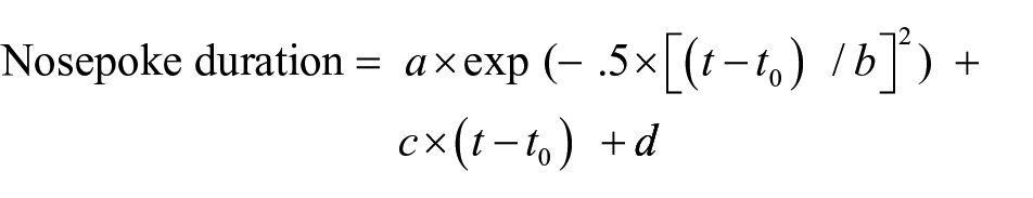
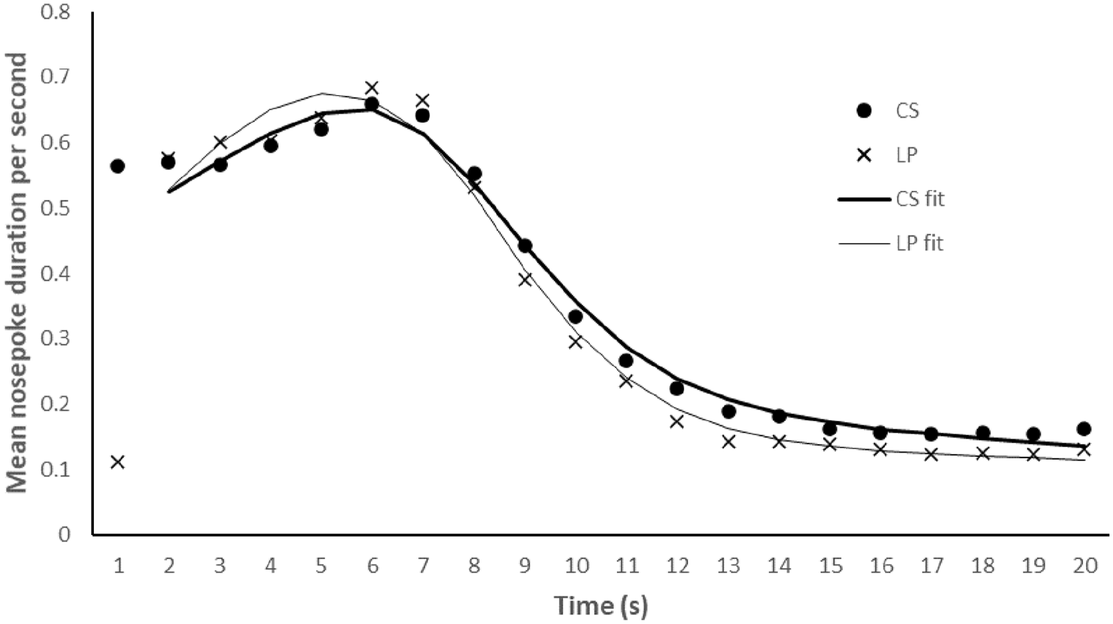
Figure 1 displays the mean rates of responding across the five test sessions for the 20-s period following the non-reinforced LP and CS. Inspection of this figure shows that in both conditions responding peaks at around 5 s, and then declines to a stable and low level by about 12 s. The mean peak response time, along with the R2 and variance in each condition, are presented in the top panel of Table 1. Inspection of this table shows that the peak response time was similar for the CS trials and LP trials, t(11) = 0.716, p = .489, SEM = 0.162. The variability of the timing peak is smaller for the LP than the CS trials, t(11) = 4.004, p = .002, SEM = 0.212. The final variable is the mean R2 value for each trial type. Inspection of these values in Table 1 indicates that the accuracy of the curve fits is generally better for the CS than the LP trials, t(11) = 2.262, p = .045, SEM = 0.007. The Bayes factors for the variance (BF10 = 21.709) and R2 (BF10 = 1.800) suggest strong and anecdotal evidence, respectively, for the alternative hypothesis that the LP values are smaller than the CS values. The Bayesian analyses for the peak time (BF10 = 0.358) provides anecdotal evidence for the null hypothesis that peak responding is the same for the CS and LP trials. Thus, we cannot conclude that there is or is not a difference in peak responding following a CS or LP. Interestingly, however, this experiment does suggest that there are differences in the way that rats respond following a CS compared with an LP, just not in terms of peak time. Inspection of Figure 1 reveals that rats did indeed respond much less in the 1-s period following an LP than a CS. This finding is readily interpreted in terms of response competition between lever pressing and nose poking, an idea that we will return to while discussing the results of Experiment 2.
Experiment 1. Mean duration (in seconds) of nose poke responding across the 20-s periods that followed the non-reinforced CS (2-s) and LP trials. The fitted curves show the mean curve fits in the CS and LP conditions from 2 s onwards.
Mean (+SEM) peak responding (s), curve fit accuracy (R2), and variance for the test data in Experiments 1 and 2.
CS: conditioned stimulus; LP: lever press.
Experiment 2
The results of Experiment 1 suggested that the peak response time was similar following an LP and a CS, but a Bayesian analyses of these results did not suggest strong support for the null hypothesis. Moreover, magazine responding 2 s following the CS was at a higher rate than following the LP, which was reflected in the larger variance on the CS trials. These observations are of potential interest: They might reflect a difference in the process of timing initiated by a LP and CS, or potentially the consequence of causal binding; albeit that a direct translation from the human causal binding literature would suggest shorter peak response times for LP trials. However, there are more prosaic analyses. It could be argued that these differences might reflect ambiguity about which components of the CS and LP served as the effective referent for the animal. For example, it seems plausible to assume that some of the variability in timing from the CS reflected differences in whether its onset or the offset was controlling timing behaviour (this could also impact on the peak time of response to the CS). In contrast, an LP and its accompanying feedback (the lever’s removal from the chamber) is perhaps more discrete. To address this possibility, Experiment 1 was replicated using a shorter CS (0.5 s). In this case, a tone served as the auditory CS because the chain of clicks created by a 0.5-s pulse of a 10-Hz clicker proved to be inconsistent.
Method
Subjects, apparatus, and procedure
16 male-hooded Lister rats were obtained from the same source and treated in the same manner as in Experiment 1. Their mean free-feeding weight was 399 g (range: 350–428 g). Rats were trained in the same operant chambers using the procedure that was described in Experiment 1, with the exception that a 0.5-s tone (3,000 Hz) was used as the CS. As with Experiment 1, rats had one pre-training session, and 5 days of testing, but were trained with the 5-s interval for 29 days before testing. Each test session consisted of 6 non-reinforced trials and 14 reinforced trials of each temporal referent.
Results and discussion
The lever was extended into the chamber for a mean 0.89 s per trial (SD = 0.33 s, range = 0.42–1.51 s). Figure 2 shows the combined data from the final 30 test trials (i.e., five sessions of training). The figure reveals that the pattern of timing was very similar for the LP and CS trials. The mean peak of responding, R2 and variance of the LP and CS trials are presented in the middle panel of Table 1. Inspection of these scores reveals that there was little difference between the peak rate of responding following a LP or CS, t(15) = 1.156, p = .266, SEM = 0.198, with anecdotal evidence for the null hypothesis, BF10 = 0.452. There was no difference in variance, t(15) = 0.256, p = .801, SEM = 0.231, with the Bayes factor providing substantial evidence for the null hypothesis, BF10 = 0.263.
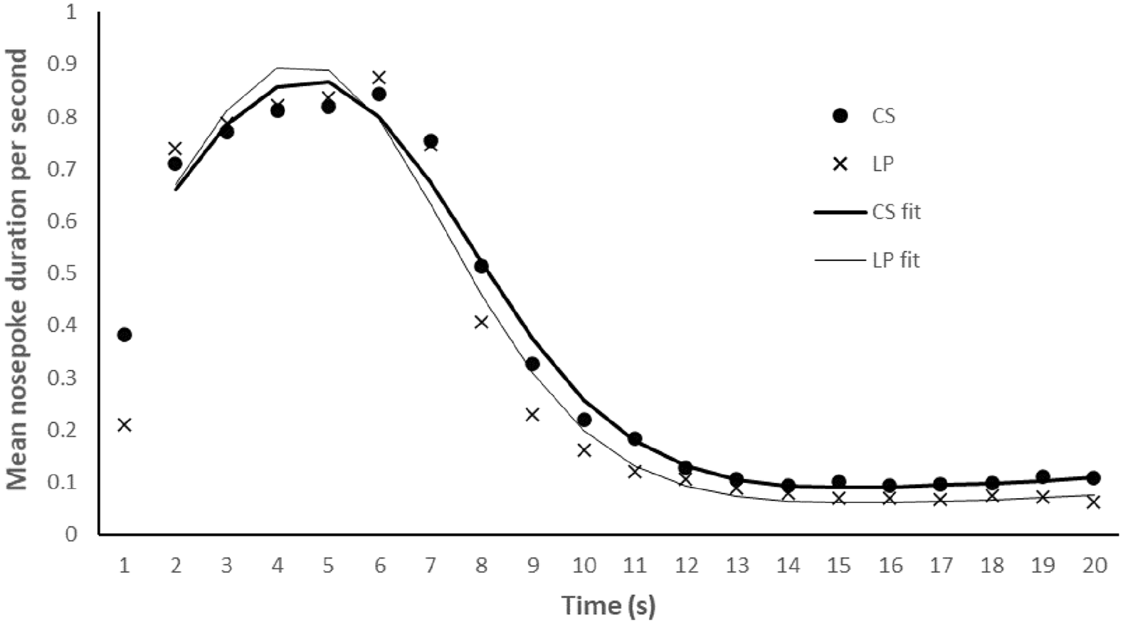
Experiment 2. Mean duration (in seconds) of nose poke responding across the 20-s periods that followed the non-reinforced CS (.5 s) and LP trials. The fitted curves show the mean curve fits in the CS and LP conditions from 2 s onwards.
The curve fits were more accurate for the CS than the LP, t(15) = 2.161, p = .047, SEM = 0.005; receiving anecdotal support by the Bayes analysis BF10 = 1.569. These results essentially replicate those of Experiment 1: There was no substantial evidence to support the conclusion that there is a difference between the LP and CS conditions, and the CS trials have more accurate curve fits. There is no difference in variance between trial types in this experiment. This finding is interesting given the attempt to make the CS condition more similar to the LP condition in terms of how long the rat had to nose poke following the stimulus onset/offset. Inspection of the data in Figure 2 suggests this difference is still present at 1 s, but responding is more similar from 2 s onwards. Thus, response competition appears to be less than in Experiment 1.
Experiment 3
Experiments 1 and 2 found no evidence for a temporal or causal binding effect: the peak rate of responding was no earlier after an action than an external cue. However, the Bayesian analyses did not reveal strong support for the conclusion that there was no effect. Experiment 3 was conducted to evaluate further the generality of the conclusion. Experiment 3 examined the mean timing from two different CS types (a 0.8-s buzzer and tone) and two LPs (to the left and right levers). The outcome for one of the referents from each type (CS1 and LP1) was food and for the other (CS2 and LP2) it was sucrose.
Method
Subjects and apparatus
16 male-hooded Lister rats were obtained from the same source and treated in the same manner as in Experiment 1. Their mean free-feeding weight was 356 g (range: 328–385 g). Rats were trained in the same operant chambers as described in the previous two experiments.
Procedure
The CSs for Experiment 3 consisted of a 0.8-s buzz (100 Hz) and 0.8-s tone (3,000 Hz) at an intensity of 80 dB. Both the left and right levers were used, leading to a total of four temporal referents. As with previous experiments, rats were given one session of pre-training, where they were presented with each trial type 10 times. One CS and one LP were immediately followed by the delivery of a food pellet, the other CS and LP were immediately followed by 0.02 mL of 20% sucrose solution. The design was fully counterbalanced. On the next 34 days, rats received training sessions which introduced a 5-s delay between CS offset or lever pressing and the outcome. Nine of each trial type was reinforced, one was non-reinforced.
Test
Rats received seven reinforced trials and three non-reinforced trials for each CS and LP. They were tested for 5 days, then retrained for 12 days (back to 1 non-reinforced trial per temporal referent), and re-tested for an additional 4 days. There was a total of 9 test days, with a total of 27 non-reinforced trials per temporal referent. This number of test days was necessary to produce more accurate curve fits, as there were fewer trials per condition in the test session compared with Experiments 1 and 2.
Analysis
To compare responding following CSs with responding following LPs, responses following each CS (i.e., CS1 and CS2) and each LP (i.e., LP1 and LP2) were pooled. The resulting mean patterns of responding for each referent type were subject to curve fitting.
Results and discussion
The lever was extended into the chamber for a mean of 2.84 s per trial (SD = 6.61 s, range = 0.26–20.06 s). Two rats had to be removed from the analysis because their curve fits were less than .80 in accuracy (both rats had poor fits for the CS and LP trials). This left a total of 14 rats for the analysis. Figure 3 shows data averaged over 9 test days (three non-reinforced trials per test day per referent). Inspection of this figure reveals similar responding for the CS and LP trials. The mean peak time, R2, and variance of the LP and CS trials are presented in the bottom panel of Table 1. Inspection of this table reveals that the peak rate of responding is similar for the CSs and LPs, t(13) = 1.115, p = .285, SEM = 0.238, which represents anecdotal evidence for the null, BF10 = 0.459. The variance was not different between the CS and LP trials, t(13) = 0.263, p = .797, SEM = 0.296, BF10 = 0.278, and the R2 was a similar accuracy for the CS and LP trials, t(13) = 0.541, p = .598, SEM = 0.009, BF10 = 0.307. Both Bayes factors provide substantial evidence for the null, and these results provide further evidence that a causal or temporal binding effect is not evident.
Experiment 3. Mean duration (in seconds) of nose poke responding across the 20-s periods following the non-reinforced CS (0.8 s) and LP trials. These data are averaged over the two types of CS and two types of LP trials. The curve fits include data from 2 s onwards.
Bayes across Experiments 1–3
Bayes factors are cumulative, therefore, we calculated the relevant overall factor across the three experiments. For peak time the Bayes factor is (BF10 = 0.358 × BF10 = 0.452 × BF10 = 0.459) = 0.074, which is strong evidence in favour of the null hypothesis. For the variance, the Bayes factor is (BF10 = 21.709 × BF10 = 0.263 ×BF10 = 0.278) = 1.587, which is anecdotal evidence for the alternative hypothesis that the CS has larger variance than the LP. Finally, for the R2 measures, the Bayes factor is (BF10 = 1.800 × BF10 = 1.569 × BF10 = 0.307) = 0.867, which is anecdotal evidence for the null hypothesis.
For the analyses presented thus far, the 1-s data point was removed from curve fitting due to the issue of response competition on the LP trials. To ensure that the removal of this time point did not impact the key result and that there is no difference between CS and LP peak time, we ran the analyses including the 1-s time point across Experiments 1–3 (see supplementary materials for descriptive statistics). Using this method, more rats had to be removed from the analysis due to poor curve fits (zero in Experiment 1, one in Experiment 2, and five in Experiment 3). Importantly, there was still evidence in favour of the null hypothesis for the peak time, as the Bayes factor is (BF10 = 1.700 × BF10 = 0.517 × BF10 = 0.306) = 0.269, so removal of the 1-s time point makes no difference to the peak rate of responding. Differences are observed, however, for the variance and R2. For the variance, the Bayes factor is (BF10 = 4.544 × BF10 = 2.789 × BF10 = 0.298) = 3.777, which is evidence for the alternative hypothesis that the CS has larger variance than the LP. The CS likely has a larger variance when 1 s is included because the rates of responding begin at a higher rate on the CS compared with the LP trials (see Figures 1 to 3). Thus, this result merely reflects the response competition associated with pressing the lever on the LP trials. For the R2 measures, the Bayes factor is (BF10 = 94.172 × BF10 = 5.045 × BF10 = 60.192) = 28,597.083, which is extreme evidence for the alternative hypothesis that the curve fits for CSs are more accurate than the LPs. The fact that accuracy is better when the 1-s time point is removed again points to the fact that responding during the 1-s time period is impacted by the trial type. This demonstrates that by removing the 1-s data point, we have removed the issue of response competition, and improved the accuracy of curve fitting.
General discussion
Animals rapidly learn that a CS (e.g., a tone) predicts the delivery of an outcome and likewise that an instrumental response (e.g., an LP) predicts an outcome. Animals can also learn when an outcome will be delivered relative to a temporal referent. Most often studies of timing in rats have used stimuli as temporal referents (but see, Caetano & Church, 2009; Lowe et al., 1974; Mechner et al., 1963), but theories of timing assume that both stimuli and responses could serve as effective temporal referents (e.g., Gibbon, 1991; Machado, 1997; for a review, see Gallistel & Gibbon, 2000). However, there is evidence to suggest that humans perceive the interval between their actions and a resulting outcome to be shorter than the interval between an external stimulus and an outcome (see Buehner & Humphreys, 2009; Haggard et al., 2002). These observations suggest that conventional stimuli and instrumental responses might differ in their capacity to serve as temporal referents for the delivery of outcomes (e.g., food). In three experiments, using within-subjects procedures, a CS (e.g., a tone) and a response (e.g., a LP) served as the referents for the start of a 5-s interval that terminated in the delivery of an outcome (food or sucrose solution). The question of interest was whether the peak rates of responding would vary as a function of the nature of the referent.
Across all three experiments, the peak times for the CS and LP trials were not different. The cumulative Bayes factor across the experiments demonstrates strong evidence for the null hypothesis. That is, there is no difference in peak time when instrumental responses and auditory stimuli serve as referents. Thus, the three experiments provided no support for the hypothesis that rats perceive the interval between an action and its resulting outcome as shorter than the interval between an external cue and its resulting outcome. While there is no direct evidence as to whether the magazine entry responses are under Pavlovian or instrumental control (and it is possible that these may differ in terms of timing), it remains the case that in at least some of the studies of binding in humans there is also performance of an action to demonstrate expectation of the outcome (e.g., Buehner & Humphreys, 2009), yet these responses show binding effects unlike in the experiments reported here. We therefore interpret these results as providing no evidence for causal binding in rats, as a belief in causality should influence behaviour to reflect the perception of temporal contiguity (Hoerl et al., 2020). This conclusion is clearly consistent with models of timing, which assume that both responses and stimuli would serve as effective referents (e.g., Gibbon, 1991; Machado, 1997). 1
The similarity in peak timing across the three experiments across different temporal referents might reflect that the offset of the stimulus and the withdrawal of the lever were equally effective temporal referents. That is, the rats were not timing from their responses, but rather from the sensory cues associated with the retraction of the lever. It is difficult to arrange that a response does not give rise to response-produced cues, which could serve as an alternative temporal referent. Moreover, Experiments 1–3 did reveal some differences in the patterns of time nose poke behaviour following the two types of temporal referent. The curve fits were more accurate for CS trials in Experiments 1 and 2, which is likely due to the increase in responding following the LP being steeper, as early responding is limited. This observation, in turn, likely reflects response competition between pressing the lever and investigating the food well. Rats cannot respond at a high level immediately following an LP as they have to move from the location of the lever to the food well to respond. In addition, the responding after the peak time is sharper for LP trials, which in turn may have affected the accuracy of curve fitting.
The variance was somewhat larger for the CS trials in Experiment 1, but similar in Experiments 2 and 3. Inspection of the spread of data in the figures appears to suggest that this might also reflect response competition in the LP condition; the initial curve is steeper from 2 to 5 s in the LP condition due to responding at 2 sec being lower. It would seem implausible to argue that lever presses can simultaneously disrupt timing based on the withdrawal of the lever, but not serve as suitable referent in their own right. In addition, the decline post-peak is slightly steeper for the LP compared with the LP trials.
Finally, while the results of Experiments 1–3 might not be surprising in the context of models of timing, in other respects the similarity in peak timing across quite different temporal referents is a striking finding. For example, it has been argued that interventions (in the shape of instrumental responses) and observations (of stimuli) differ in their access to the process of causal reasoning, with interventions having a privileged status (e.g., Leising et al., 2008). The results of Experiments 1–3 provide no evidence for such privileged access to the mechanisms that underlie timing behaviour in rats—no evidence of temporal or causal binding. These results join others (e.g., Burgess et al., 2012; Dwyer et al., 2009) in suggesting that it is premature to suggest that interventions and observations have a fundamentally different status in rats.
Supplemental Material
sj-docx-1-qjp-10.1177_17470218221090418 – Supplemental material for Instrumental responses and Pavlovian stimuli as temporal referents in a peak procedure
Supplemental material, sj-docx-1-qjp-10.1177_17470218221090418 for Instrumental responses and Pavlovian stimuli as temporal referents in a peak procedure by Katy V Burgess, Robert C Honey and Dominic M Dwyer in Quarterly Journal of Experimental Psychology
Footnotes
Declaration of conflicting interests
The author(s) declared no potential conflicts of interest with respect to the research, authorship, and/or publication of this article.
Funding
The author(s) received no financial support for the research, authorship, and/or publication of this article.
Notes
References
Supplementary Material
Please find the following supplemental material available below.
For Open Access articles published under a Creative Commons License, all supplemental material carries the same license as the article it is associated with.
For non-Open Access articles published, all supplemental material carries a non-exclusive license, and permission requests for re-use of supplemental material or any part of supplemental material shall be sent directly to the copyright owner as specified in the copyright notice associated with the article.