Sage Journals: Discover world-class research

Abstract

Governments around the world are regulating the thermal performance of new and retrofitted dwellings to reduce the significant energy demand for space heating. These efforts are undermined by case-study evidence of a significant performance gap between the thermal performance predicted for compliance and the thermal performance that is achieved in-use. Overall building thermal performance is most simply described by the Heat Transfer Coefficient (HTC) metric. New low-cost methods are being developed to measure the in-use HTC of dwellings, that is, measured during occupancy. If deployed at scale, these methods could provide much-needed evidence of the performance gap and help to close it through feedback and quality assurance. This paper quantifies, for the first time, the variability in repeated measurements of the in-use HTC of occupied dwellings over a winter heating season and demonstrates that this variability can be explained by changes in the average boundary conditions (indoor air temperatures and weather). This finding could provide measurements of the in-use HTC with a higher precision than when the variability is simply assumed to be part of the uncertainty in the measurement. The in-use HTC of 19 occupied dwellings was repeatedly calculated over rolling 20-day periods for up to 6 months. The in-use HTC of the dwellings had a coefficient of variation (standard deviation divided by mean) of between 1.0% and 11.8% (mean 7.1%). Valid linear models that described the variability in the in-use HTC (dependent variable) by considering variations in the boundary conditions at the time of each repeated measurement (independent variables) were created for 17 of the 19 dwellings. The in-use HTC for each dwelling had a unique relationship with the boundary conditions and required a unique linear model. The linear model explained at least 80% of the variability in 13 of 17 dwellings.

Keywords

building thermal performance heat transfer coefficient in-use measurement occupied dwellings variability

Introduction

The International Energy Agency identify that more effort is needed to reduce the significant use of fossil fuels for space heating in buildings (IEA, 2023c). Across the UK, the domestic sector consumes 29% of all energy supplied (BEIS, 2020a), with around three-quarters of this energy used for space heating (BEIS, 2020b). The space-heating energy demand of UK dwellings must be drastically reduced if the domestic sector is to decarbonise and support the UK’s legally binding commitment to reach net zero greenhouse gas emissions by 2050 (HM Government, 2020).

Globally, energy efficiency has been identified as a relatively quick and cost-effective way to reduce CO₂ emissions, lower energy bills and strengthen energy security (IEA, 2023b). Reducing the heat loss from the building envelope is the most effective way to reduce space heating energy demand (IEA, 2023a). The UK has some of the oldest and least thermally efficient dwellings in the world (Piddington et al., 2020). Higher thermal performance standards of new dwellings are mandated through the regular updates to the Building Regulations (Part L) (HM Government, 2021a). The UK Government are investing in improving the thermal performance of existing dwellings through large-scale insulation schemes such as the Great British Insulation Scheme (GBIS) (Ofgem, 2023), Green Homes Grants (GHG) (HM Government, 2021c) and the Energy Company Obligation (ECO) (Ofgem, 2022).

The thermal performance of dwellings can be quantified by the Heat Transfer Coefficient (HTC). The HTC describes the spatio-temporal average rate of heat loss through the building envelope, including infiltration and ventilation,¹ in units of watts per °C temperature difference between indoor air and outdoor air (commonly used SI units are W/K (BSI, 2017b), and this is equivalent to W/°C; W/ºC are used in this paper to make the HTC more universally understandable as a metric). The HTC can be derived in different ways including calculated values based on models, bespoke HTC measurement tests undertaken in unoccupied dwellings, and unobtrusive in-use HTC measurements in occupied dwellings.

The HTC is calculated as part of the UK Government’s National Calculation Methodology – the Standard Assessment Procedure (SAP) – for assessing the energy performance of new and existing dwellings (BRE, 2022) and therefore underpins policy, including building regulations and Energy Performance Certificates (EPCs). The calculation is based on summing the expected thermal performance of individual building elements, based on their construction materials (as explained in section ‘Calculating the HTC and its variability’). This calculated HTC is hereafter called the SAP HTC.

The HTC can be measured in unoccupied dwellings using, for example, the aggregate heat loss test (BSI, 2024) and the Quick U-Building test (QUB, Alzetto et al., 2018). The aggregate heat loss test, previously called the co-heating test (Johnston et al., 2013), takes around 3 weeks at a constant elevated indoor air temperature of around 21°C–25°C. The QUB uses a constant heating phase followed by a period of free-cooling to measure the HTC in just one night (Alzetto et al., 2018). These methods require significant resources (knowledge, equipment and cost) to undertake (Senave et al., 2019), but their use has transformed our understanding of the thermal performance of dwellings and identified a thermal performance gap between the measured and SAP HTC (e.g. Johnston et al., 2015; Marshall et al., 2017; Wingfield et al., 2011; Zero Carbon Hub, 2014).

The thermal performance gap between the measured and SAP HTC is unsurprising, as the SAP HTC is calculated at a single point in time using assumed construction properties, thereby failing to recognise that: the construction of dwellings varies in materials and quality, materials and construction may degrade over time, and dwellings can be subsequently altered in many ways that affect thermal performance (including energy efficiency retrofits such as insulation and draught proofing). The SAP HTC should not be expected to be an accurate prediction of the thermal performance of an individual dwelling.

The thermal performance gap is problematic because dwellings may not perform as well as expected and this undermines the credibility of policy aimed at improving the thermal performance. Imposing tighter regulation on the construction and retrofit of dwellings, and funding efforts to improve thermal performance, may fail to deliver the expected outcomes if there is no quality control measurement. Households risk being left with underperforming homes that are thermally uncomfortable and/or expensive to heat.

To address these problems international teams of scientists and engineers have collaborated to develop low-cost methods to measure the thermal performance of dwellings at scale while they are occupied, that is, the in-use HTC (e.g. Bauwens et al., 2021; IEA EBC, 2024). Routinely measuring the in-use HTC of dwellings has the potential to revolutionise their performance by, for example, enabling routine quality control of construction and refurbishment for regulation and private finance, providing feedback into the design and construction processes, improving the targeting of badly performing dwellings, providing households with accurate energy demand predictions and simplifying the accurate sizing of retrofit heat pumps.

A method for measuring the in-use HTC was proposed a decade ago (Jack, 2015). The UK Government accelerated the commercial adoption of in-use HTC through an innovation competition which funded the development and evaluation of nine different Smart Meter Thermal Efficiency Rating (SMETER) methods (HM Government, 2022). There were variations between the nine methods, but most used indoor air temperature sensors and smart meter data, along with data from a nearby weather station, to calculate the HTC (Allinson et al., 2022). The best of these methods were more accurate than the SAP HTC, and households found the installed sensors to be unobtrusive (ibid). Improving the accuracy of these methods further will help to improve confidence in their application and accelerate widespread adoption.

The value of the HTC can vary depending on when it is measured. For example, the UK Government’s National Calculation Methodology for assessing the energy performance of dwellings – SAP for new dwellings and the reduced data version, RdSAP, for existing dwellings (BRE, 2022) – specifies monthly values of the SAP HTC that are calculated from monthly averages of the wind speed to account for the resulting changes in ventilation and infiltration heat losses. BS EN ISO 13370:2017 also considers monthly values but based on assumptions about changes to the temperature of the ground beneath the building (BSI, 2017a). Other boundary conditions at the time of measurement, including the air temperature indoors and outdoors and the wind speed and direction, have been shown to have impact on the HTC (e.g. see Juricic et al., 2021; Li, 2022; Stamp, 2015) but these findings were based on computer simulations rather than measurements. For example, the HTC of a dwelling has been shown to vary with changes in outdoor conditions (Stamp, 2015). When conducting short duration (2–3 days) HTC measurement tests in unoccupied dwellings, including the Sereine test, QUB and ISABELE (Juricic et al., 2023; Sougkakis et al., 2021; Thébault and Bouchié, 2018), variability in the measured HTC values due to different boundary conditions was treated as a source of uncertainty. To the authors’ knowledge, there is no reliable evidence of the magnitude of the variability of the in-use HTC, and no-one has proposed ways to account for this variability in practice other than including it in the combined uncertainty.

Li (2022) proposed that the difference between two HTC values cannot only be attributed to measurement uncertainty, but also variability in the HTC due to non-random changes in the boundary conditions of the dwelling. Variability could explain changes in the HTC due to factors including: varying wind speed and direction which can impact the infiltration rate of a dwelling; changes in indoor and outdoor temperature which can alter the surface resistances due to buoyancy effects in addition to infiltration; and the impact of solar radiation on heat transfer through opaque elements (Gori et al., 2023). Crucially, this paper presents the first attempt to quantify the variability of the HTC using data collected from occupied dwellings and proposes a method to account for this variability.

This paper aims to improve the precision of measurements of the in-use thermal performance of dwellings by using a novel method which accounts for the variability in the in-use HTC that is caused by changes in the boundary conditions at the time of the measurement. The in-use HTC of 19 dwellings was repeatedly calculated over rolling 20-day periods (days 1–20, days 2–21, days 3–22, etc.) for up to 6 months to quantify the magnitude of the variability. Linear models that describe the variability in the HTC as a function of the boundary conditions during the measurement period were created. This paper, therefore, evaluates an important and original way to reduce the uncertainty in in-use HTC measurements and help accelerate routine in-use measurement to close the performance gap and support the global decarbonisation of dwellings.

Methods

The work in this paper is underpinned by data collected from 19 dwellings. The in-use HTC was calculated from the data for each dwelling to understand the variability in its value. Linear models of the in-use HTC (dependent variable) were created to explain the variability using the average boundary conditions during each measurement period (independent variables). The linear models were used to predict the in-use HTC at a defined set of boundary conditions and evaluate whether this could explain the variability and thereby reduce the uncertainty.

Dataset

Data collected from 19 occupied dwellings in North West England, recorded as part of the Technical Evaluation of SMETER Technologies (TEST) Project Phase 2 (Allinson et al., 2022, 2024), were used for the analysis in this paper. The 19 dwellings were a sub-set of 30 that were monitored during that project (Table 1), in which two did not have a valid aggregate heat loss test and another nine had insufficient data to calculate at least 10 in-use HTC values during the winter heating season (as described in Section ‘Calculating the HTC and its variability’). The aggregate heat loss test results were required for comparisons and at least 10 in-use HTC results were required for the linear model, as described in Section ‘Creating linear models to explain the variability in the in-use HTC’.

Table 1.

19 of the 30 dwellings in the TEST project dataset were used for the analysis in this paper – two dwellings were excluded as they did not have a valid aggregate heat loss test and nine were excluded as there was insufficient monitored data to calculate at least 10 in-use HTC values (excluded dwellings are greyed-out, bold text denotes the reason for exclusion).

Dwelling	Aggregateheat losstest start date(duration in days)	Aggregate heatloss test HTC(W/°C)	In-use HTCstart date	Numberof in-useHTC values	AverageRdSAP HTC(W/°C)	Difference betweenRdSAP andaggregate heatloss test HTC^a
HH01	21/3/19 (14)	181	3/3/20	2
HH02	21/4/19 (12)	131	21/2/20	2
HH03	30/4/19 (17)	155	8/3/20	2
HH04	24/9/19 (9)	153	26/11/19	26	147	−4%
HH05		None
HH06	3/10/19 (11)	212	26/11/19	12	334	58%
HH07		None
HH08	10/10/19 (10)	213	26/11/19	20	230	8%
HH09	4/10/19 (7)	172	26/11/19	19	165	−4%
HH10	12/10/19 (11)	194	26/11/19	1
HH11	19/10/19 (16)	213	26/11/19	13	209	−2%
HH12	23/10/19 (16)	127	26/11/19	14	141	11%
HH13	7/11/19 (8)	159	26/11/19	52	150	−6%
HH14	15/11/19 (7)	137	26/11/19	8
HH15	7/11/19 (11)	208	26/11/19	30	180	−13%
HH16	7/11/19 (18)	184	12/12/19	17	176	−4%
HH17	21/11/19 (7)	191	12/12/19	26	164	−14%
HH18	14/11/19 (19)	148	12/12/19	29	146	−1%
HH19	15/11/19 (14)	155	12/12/19	49	172	11%
HH20	22/11/19 (14)	229	12/12/19	13	200	−13%
HH21	24/11/19 (16)	269	18/12/19	42	234	−13%
HH22	4/12/19 (6)	194	12/12/19	2
HH23	5/12/19 (11)	237	16/1/20	14	219	−8%
HH24	28/11/19 (13)	171	31/1/20	11	145	−15%
HH25	9/12/19 (10)	244	31/1/20	14	192	−21%
HH26	5/12/19 (12)	254	31/1/20	12	204	−20%
HH27	25/12/19 (13)	201	31/1/20	14	208	3%
HH28	20/12/19 (16)	172	31/1/20	7
HH29	6/2/20 (11)	226	28/2/20	2
HH30	4/2/20 (11)	227	4/3/20	2

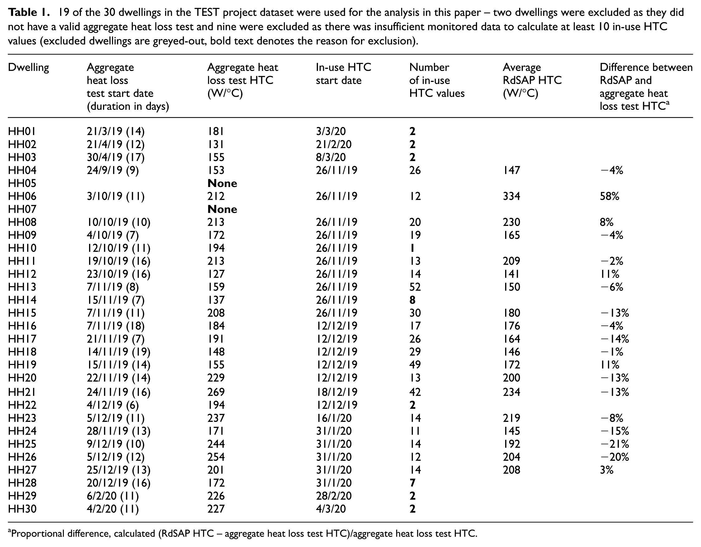
Proportional difference, calculated (RdSAP HTC – aggregate heat loss test HTC)/aggregate heat loss test HTC.

All of the aggregate heat loss tests² were carried out in unoccupied dwellings, a household then moved in and monitoring for in-use HTC started – the dates of the testing and monitoring were different for each dwelling (Table 1) (Allinson et al., 2024). The dataset included the aggregate heat loss test HTC, and the SAP HTC predicted by the reduced data version of the UK Government’s National Calculation Methodology for assessing the energy performance of dwellings, RdSAP, based on a survey of the dwelling (BRE, 2022). The thermal performance gap for these dwellings, based on the difference between the average (October to March) RdSAP prediction and the aggregate heat loss test result, ranged from −21% to +58% (Table 1). This was calculated by dividing the difference between the SAP HTC and aggregate heat loss test HTC by the aggregate heat loss test result. The data collected while the dwellings were occupied included: gas and electricity consumption from smart meters (±1% accuracy) recorded every 30 minutes; indoor air temperatures (±0.2°C) in most rooms recorded every 30 minutes; and outdoor air temperature (±0.3°C), wind speed (±3% at 10 m/s), wind direction (±3°) and vertical south-facing solar irradiance (±10%), at 10-minute intervals (Allinson et al., 2022, 2024).

Calculating the HTC and its variability

The in-use HTC was calculated for each dwelling in the dataset, over rolling 20-day periods, using all available data until the end of March 2020 (end of the main heating season). Results from any 20-day periods where the average indoor-outdoor temperature difference was less than 10°C were removed from further analysis to reduce uncertainties caused by low rates of heat loss (as recommended by Johnston et al., 2013). There were between 2 and 52 valid in-use HTC results for each dwelling (Table 1). Any dwellings with fewer than 10 in-use HTC results were removed from further analysis as a minimum of 10 in-use measurements were required for constructing the linear models described in Section ‘Creating linear models to explain the variability in the in-use HTC’.

The in-use HTC was calculated using the multiple linear regression method, as described by Bauwens and Roels (2014), expressed as equation (1):

Heating power (W) = HTC ({W /}^{°} C) \times Δ T (^{°} C) - solar aperture (m^{2}) \times s o l a r i r r a d i a n c e (W / m^{2})

(1)

For each 20-day period, daily mean whole-dwelling heating power (W) was regressed on daily mean south-facing vertical solar irradiance (W/m²) and indoor-outdoor air temperature difference $Δ T$ (°C) (with daily means calculated from midnight to midnight). Daily mean heating power was the sum of daily mean electrical power and gas power, which were derived from dwelling smart meter monitoring data.³ The solar aperture represents the equivalent area (m²) of a fully transparent vertical opening for solar heat gains and is solved by the regression alongside HTC.

The SAP HTC was calculated for each dwelling in the dataset using the RdSAP formulation (BEIS, 2019):

SAP HTC (W /^{°} C) = Σ_{i} (U_{i} \times A_{i}) + (0.15 \times A) + \frac{1}{3} nVf

(2)

where:

U_i is the U-value of the i^th planar building envelope element (W/m².ºC)

A_i is the area of the i^th planar building envelope element (m²)

∑_i is the sum over all planar building envelope elements

0.15 is a thermal bridging factor (W/m².ºC), added to account for the additional heat loss due to thermal bridges, for example, around windows and at the point where elements join (ibid)

A is the total exposed envelope area (m²)

n is the air changes per hour (h⁻¹)

V is the building volume (m³)

f is a factor to account for the sheltering of the subject dwelling by surrounding buildings and monthly variations in wind speed.

The SAP HTC is therefore different for every month of the year as the wind speed varies. Only the SAP HTCs calculated for the winter period (October to March inclusive) were used in this analysis.

For each dwelling, the coefficient of variation (COV) of the in-use HTC was calculated by dividing the sample standard deviation (SD) by the mean in-use HTC (equation (3)). 95% confidence intervals for the mean in-use HTC for each dwelling were calculated in accordance with BS 2846-2:1981 (BSI, 1981), based on the number of 20-day values of the in-use HTC calculated for a given dwelling. For the confidence intervals to be valid, the HTC values must approximate a normal distribution, determined using the method presented in Section ‘Creating linear models to explain the variability in the in-use HTC’.

The COV and 95% confidence intervals of the SAP HTC were calculated for each dwelling in the same way using the six SAP HTC values for each month of the main heating season October to March.

Coefficient of variation, COV = \frac{SD}{HT C_{mean}}

(3)

Creating linear models to explain the variability in the in-use HTC

Stepwise regression analysis was used to create a linear model for each dwelling, relating the in-use HTC for each 20-day period (dependent variable) to the average boundary conditions observed during that period (independent variables). The analysis was conducted using SPSS Statistics (Version 29.0.2.0) (IBM Corp, 2023). Stepwise regression is a form of hierarchical regression which is best suited to multiple independent variables, due to its ability to select the most important variables in the linear model, and to exclude those variables which are not important to the linear model (IBM, 2023b).

The model considered the following boundary conditions (as identified by Li, 2022; Stamp, 2015), averaged over each 20-day period, as the independent variables:

Mean indoor air temperature, Ti (°C)

Mean outdoor air temperature, To (°C)

Mean indoor-outdoor temperature difference, ΔT (°C)

Mean solar irradiance incident on a south-facing vertical surface, VS (W/m²)

Mean wind speed, Ws (m/s)

Mean wind direction, Wd (°)

Mean easting components of wind direction, Wu (m/s)⁴

Mean northing components of wind direction, Wv (m/s)

Huta (2014) proposed a minimum sample of K + 2, where K is the number of independent variables to be used in hierarchical linear regression. As up to eight independent variables are used in the analysis presented, a minimum sample of ten in-use HTC results was imposed.

For a linear model to be deemed valid, it must adhere to four assumptions: linearity, independence, normality of residuals and homoscedasticity (Knief and Forstmeier, 2021). Boundary conditions (independent variables) were only included in the stepwise regression analysis when the correlation with the HTC (dependent variable) was considered sufficiently strong, as indicated by a correlation coefficient r with magnitude |r| > 0.2 after the literature (Miles and Shevlin, 2001; Morris, 2013). To limit any collinearity, pairs of independent variables were only included when |r| ≤ 0.7 when a line of regression was plotted for each pair of variables; for pairs of variables with |r| > 0.7, a maximum of one variable was included in the analysis after the rule of thumb set out by Allison (1999) and Miles and Shevlin (2001). Independent variables were only added to the stepwise regression model when they were deemed to be significant predictors, having a p-value less than 0.05, that is, there is at least a 95% likelihood that the result is not due to chance (IBM, 2023a). To demonstrate the normality of residuals, the skewness and the excess kurtosis of the residuals were examined (excess kurtosis is a measure of how far from ‘normal’ the kurtosis is). Upper limits of ±2.0 for skewness and excess kurtosis were chosen (George and Mallery, 2020; Mishra et al., 2019). Finally, the homoscedasticity of the linear model was checked by plotting the residuals against the predicted values (Morris, 2013). The linear model was deemed to be homoscedastic if the variation of the points around the line of regression was constant (Marill, 2004), that is, there was no clear pattern or correlation evident in the plots. Only those linear models which met the above criteria were deemed valid.

Predicting the in-use HTC for specific boundary conditions

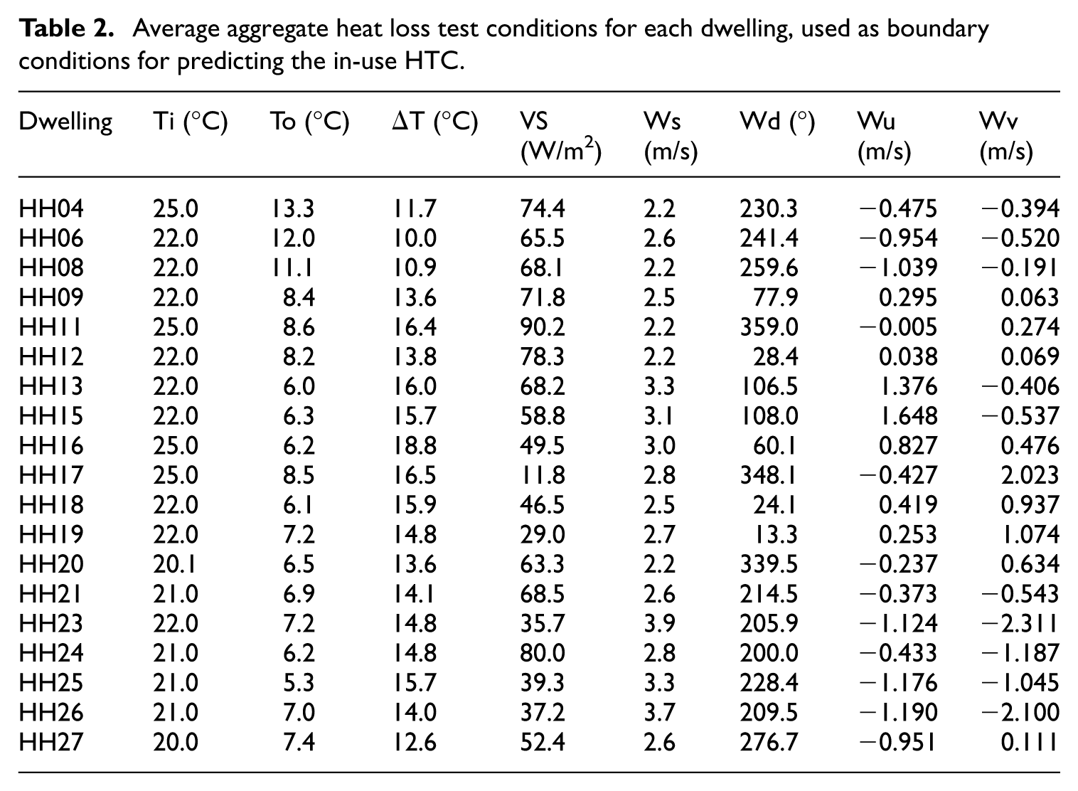
The linear models for each dwelling were used to predict the in-use HTC under average aggregate heat loss test conditions (Table 2). These represent the mean of each boundary condition recorded during the aggregate heat loss test for each dwelling and could enable the in-use HTC of any dwelling to be better compared with the aggregate heat loss test HTC.

Table 2.

Average aggregate heat loss test conditions for each dwelling, used as boundary conditions for predicting the in-use HTC.

Dwelling	Ti (°C)	To (°C)	ΔT (°C)	VS(W/m²)	Ws(m/s)	Wd (°)	Wu(m/s)	Wv(m/s)
HH04	25.0	13.3	11.7	74.4	2.2	230.3	−0.475	−0.394
HH06	22.0	12.0	10.0	65.5	2.6	241.4	−0.954	−0.520
HH08	22.0	11.1	10.9	68.1	2.2	259.6	−1.039	−0.191
HH09	22.0	8.4	13.6	71.8	2.5	77.9	0.295	0.063
HH11	25.0	8.6	16.4	90.2	2.2	359.0	−0.005	0.274
HH12	22.0	8.2	13.8	78.3	2.2	28.4	0.038	0.069
HH13	22.0	6.0	16.0	68.2	3.3	106.5	1.376	−0.406
HH15	22.0	6.3	15.7	58.8	3.1	108.0	1.648	−0.537
HH16	25.0	6.2	18.8	49.5	3.0	60.1	0.827	0.476
HH17	25.0	8.5	16.5	11.8	2.8	348.1	−0.427	2.023
HH18	22.0	6.1	15.9	46.5	2.5	24.1	0.419	0.937
HH19	22.0	7.2	14.8	29.0	2.7	13.3	0.253	1.074
HH20	20.1	6.5	13.6	63.3	2.2	339.5	−0.237	0.634
HH21	21.0	6.9	14.1	68.5	2.6	214.5	−0.373	−0.543
HH23	22.0	7.2	14.8	35.7	3.9	205.9	−1.124	−2.311
HH24	21.0	6.2	14.8	80.0	2.8	200.0	−0.433	−1.187
HH25	21.0	5.3	15.7	39.3	3.3	228.4	−1.176	−1.045
HH26	21.0	7.0	14.0	37.2	3.7	209.5	−1.190	−2.100
HH27	20.0	7.4	12.6	52.4	2.6	276.7	−0.951	0.111

For each dwelling, the in-use HTC was predicted for the set of defined boundary conditions using equation (4). The accuracy of the predicted HTC was quantified using the coefficient of variation of the root mean square error (CVRMSE), calculated using equation (5).

HT C_{predicted} = constant + coef f_{1} \cdot B C_{1} + coef f_{2} \cdot B C_{2} + \dots + coef f_{n} \cdot B C_{n}

(4)

where:

coeff _n is the regression coefficient for the $n^{th}$ boundary condition, taken, along with the constant, from the corresponding linear model (Table 5).

BC _n is the value of the $n^{th}$ boundary condition used to predict the in-use HTC (Table 2).

CVRMSE = \frac{1}{\hat{H}} \sqrt{\frac{\sum {(H_{AHLT, i} - H_{in - use, i})}^{2}}{N}}

(5)

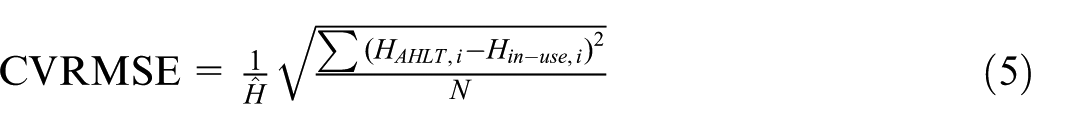
where:

H_AHLT,i is the aggregate heat loss test HTC for the i^th dwelling in the sample (W/°C)

H_in-use,i is the in-use HTC for the i^th dwelling in the sample (either in-use HTC or in-use HTC predicted for average aggregate heat loss test conditions) (W/°C)

$\hat{H}$ is the average of the aggregate heat loss test HTC and in-use HTC for all dwellings in the sample (W/°C)

N is the sample size

Results

The variability, as defined by the coefficient of variation, of the in-use HTC was calculated for each dwelling. Linear models were created for the in-use HTC of each dwelling to explain the variability due to the boundary conditions. The in-use HTC of each dwelling was predicted for a set of boundary conditions.

Variability in the HTC

The in-use HTC, calculated using 20-day rolling periods between October 2019 and March 2020 (where data were available), had a coefficient of variation (COV = standard deviation divided by mean) of between 1.0% and 11.8%, with an average COV of 7.1% (Table 3, Figure 1). The distribution of in-use HTC values for each dwelling could be approximated by a normal distribution.⁵ The 95% confidence interval for the mean in-use HTC, based on the repeated 20-day periods was between 0.6% and 6.8%, with a mean of 3.4%.

Table 3.

Variability of in-use HTC based on N results from 20-day rolling periods between October and March. Standard deviation (SD) calculated for the sample, alongside coefficient of variation (COV) and 95% confidence intervals (CI).

Dwelling	In-use HTC (W/ºC)
	N	Range of values	Mean	SD	COV (%)	95% CI (±% of mean, %)
HH04	26	134.8–152.1	145.7	4.3	2.9	±1.2
HH06	12	255.8–263.6	259.9	2.6	1.0	±0.6
HH08	20	218.3–271.6	247.0	21.5	8.7	±4.1
HH09	19	142.8–171.6	160.8	9.5	5.9	±2.8
HH11	13	212.3–297.7	271.6	26.0	9.6	±5.8
HH12	14	119.5–152.6	142.5	10.0	7.0	±4.1
HH13	52	124.2–177.2	152.9	12.7	8.3	±2.3
HH15	30	148.5–221.1	191.3	19.8	10.3	±3.9
HH16	17	140.8–187.1	172.0	15.4	9.0	±4.6
HH17	26	139.7–215.8	168.9	19.9	11.8	±4.7
HH18	29	133.6–177.4	161.5	12.3	7.6	±2.9
HH19	49	118.1–177.5	153.0	14.3	9.4	±2.7
HH20	13	191.2–217.2	203.9	8.6	4.2	±2.6
HH21	42	265.8–310.2	291.3	12.5	4.3	±1.3
HH23	14	186.1–248.3	231.1	17.4	7.5	±4.3
HH24	11	152.5–205.5	191.8	19.4	10.1	±6.8
HH25	14	166.3–215.3	202.3	16.0	7.9	±4.6
HH26	12	244.2–254.5	249.3	3.6	1.5	±0.9
HH27	14	161.2–214.9	203.6	17.7	8.7	±5.0

Figure 1.

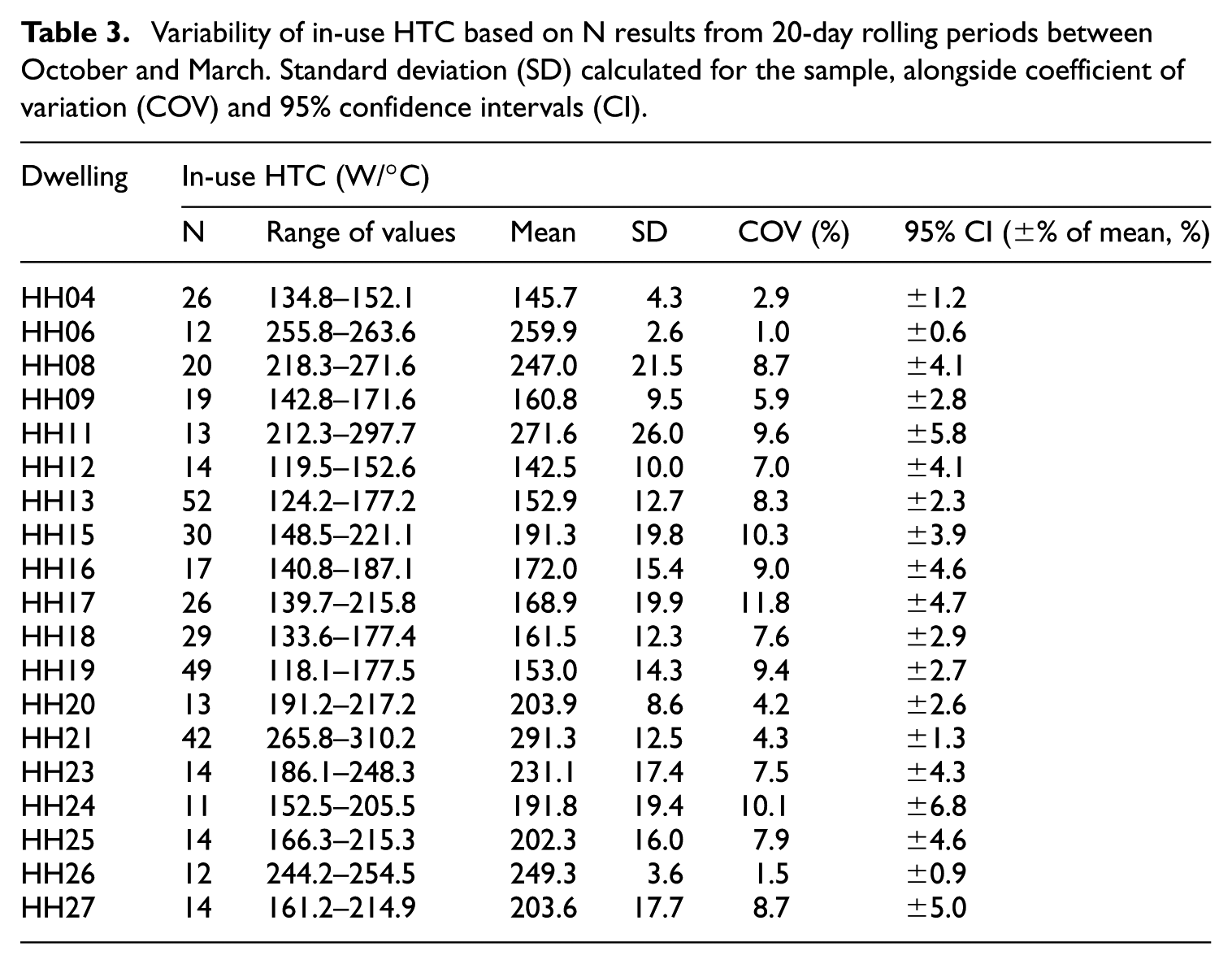
In-use HTC using 20-day rolling periods across the monitoring period (October 2019 to March 2020, inclusive) for all dwellings in the sample.

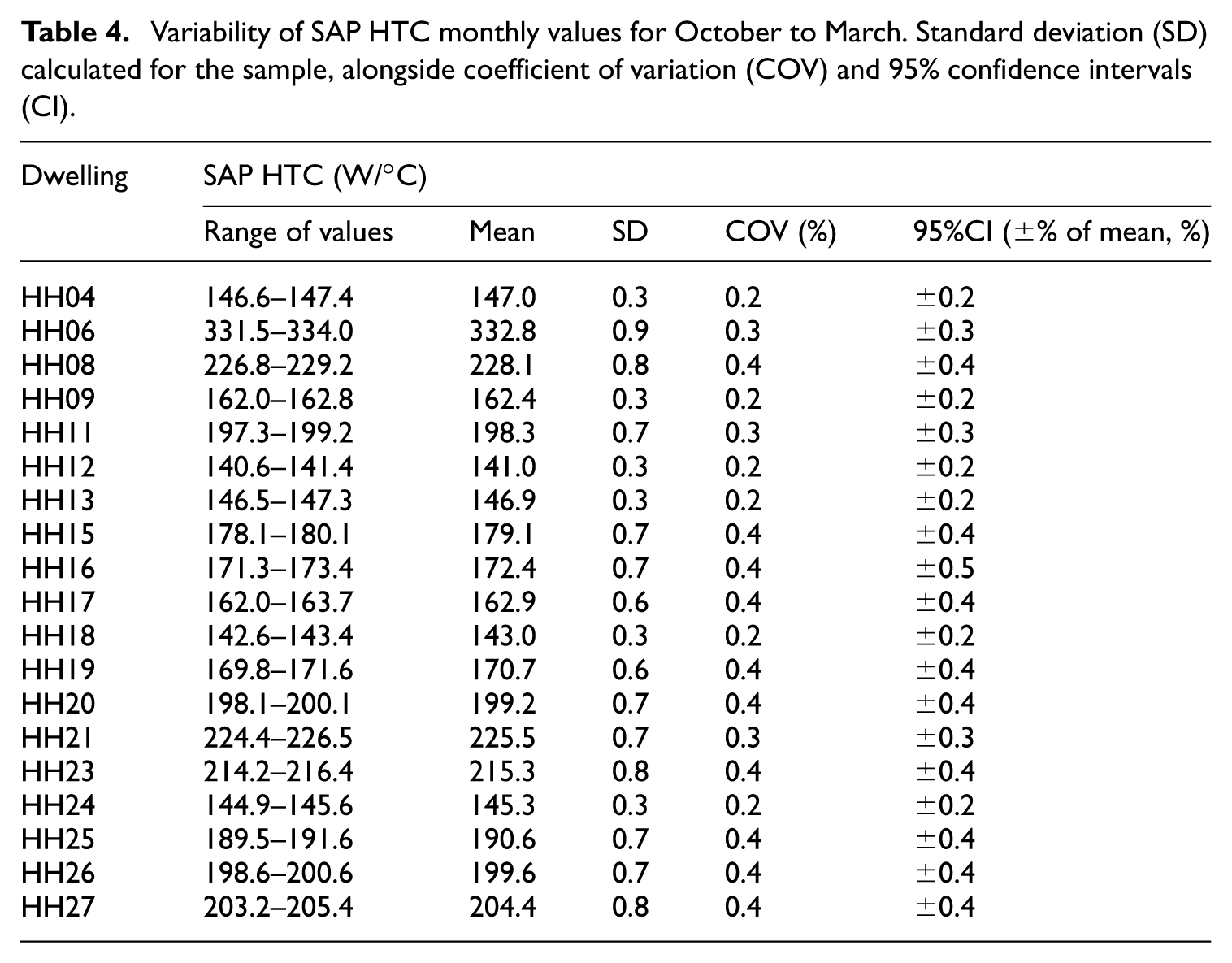
Using monthly mean values between October and March, inclusive, SAP HTC had a COV of between 0.2% and 0.4% (Table 4). 95% confidence intervals for the mean SAP HTC were between 0.2% and 0.5%. SAP only considers wind speed in the monthly values of the HTC, so understanding the variability that is due to other boundary conditions is important, that is, the SAP HTC could be better corrected to account for other sources of variability.

Table 4.

Variability of SAP HTC monthly values for October to March. Standard deviation (SD) calculated for the sample, alongside coefficient of variation (COV) and 95% confidence intervals (CI).

Dwelling	SAP HTC (W/ºC)
	Range of values	Mean	SD	COV (%)	95%CI (±% of mean, %)
HH04	146.6–147.4	147.0	0.3	0.2	±0.2
HH06	331.5–334.0	332.8	0.9	0.3	±0.3
HH08	226.8–229.2	228.1	0.8	0.4	±0.4
HH09	162.0–162.8	162.4	0.3	0.2	±0.2
HH11	197.3–199.2	198.3	0.7	0.3	±0.3
HH12	140.6–141.4	141.0	0.3	0.2	±0.2
HH13	146.5–147.3	146.9	0.3	0.2	±0.2
HH15	178.1–180.1	179.1	0.7	0.4	±0.4
HH16	171.3–173.4	172.4	0.7	0.4	±0.5
HH17	162.0–163.7	162.9	0.6	0.4	±0.4
HH18	142.6–143.4	143.0	0.3	0.2	±0.2
HH19	169.8–171.6	170.7	0.6	0.4	±0.4
HH20	198.1–200.1	199.2	0.7	0.4	±0.4
HH21	224.4–226.5	225.5	0.7	0.3	±0.3
HH23	214.2–216.4	215.3	0.8	0.4	±0.4
HH24	144.9–145.6	145.3	0.3	0.2	±0.2
HH25	189.5–191.6	190.6	0.7	0.4	±0.4
HH26	198.6–200.6	199.6	0.7	0.4	±0.4
HH27	203.2–205.4	204.4	0.8	0.4	±0.4

The observed variability in the in-use HTC is comparable with simulations of aggregate heat loss tests conducted over the duration of a winter, where Stamp (2015) observed COV values between 2.8% and 11.7% for four identical dwellings with varying airtightness.

Linear models to explain the variability

The relationship between the in-use HTC and the boundary conditions at the time of the measurement varied between dwellings. For the indoor air temperature (Ti), the magnitude |r| of the correlation coefficient ranged between 0.047 and 0.996; and for outdoor air temperature (To), |r| ranged between 0.010 and 0.972 (Figure 2). Similar ranges of |r| were observed for all other boundary conditions. Boundary conditions with a low correlation coefficient were not selected for the linear model.

Figure 2.

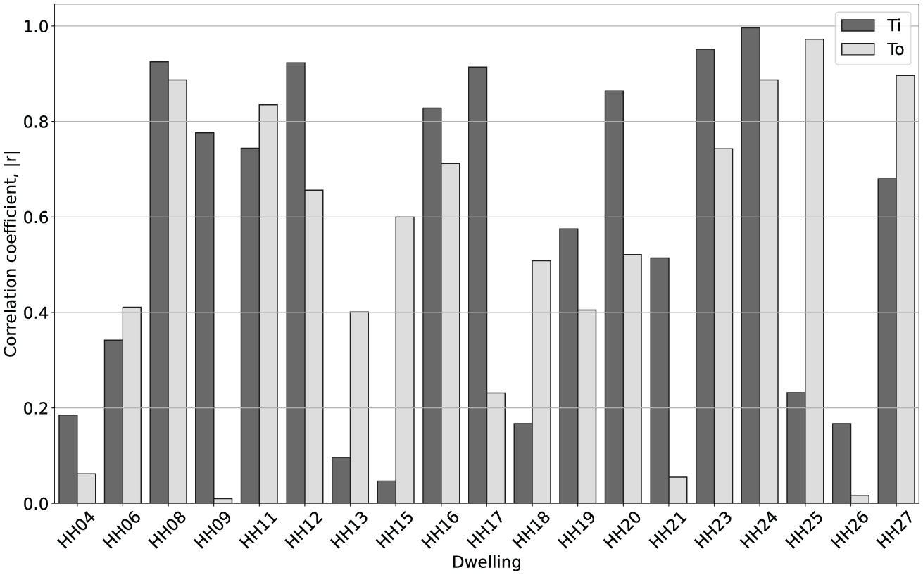
Correlations between the in-use HTC and the indoor and outdoor air temperatures.

Valid linear models were created for 17 of the 19 dwellings. There were no combinations of independent variables which formed a statistically significant linear model (p-value less than 0.05 in F-test for overall model significance) for HH06 and HH26 and they were removed from further analysis. The F-statistics of the models for each of the remaining 17 dwellings were all greater than 1 (minimum 9.5, maximum 1243.8), whilst the corresponding p-value for each model was <0.001 in all cases, demonstrating statistical significance in the linear models (George and Mallery, 2020).

The linear models used between one and four of the eight possible boundary conditions; each one of the eight was chosen by at least one model, but there was no consistency in which boundary conditions were chosen (Table 5). The most commonly used boundary conditions were wind u-component (Wu – nine times across the 17 models), indoor air temperature (Ti – six times) and outdoor air temperature (To – five times). The sign (positive or negative) of the regression coefficients for most boundary conditions varied; however, for wind speed (Ws) it was always positive, as might be expected: higher wind speed produces a higher rate of heat loss and therefore a higher HTC. It is hypothesised that Wu was used most due to the prevailing winds from the west.

Table 5.

The linear model for each dwelling as identified by the stepwise regression, including coefficient of determination (r²) and standard error of the estimate (Std. Error).

Dwelling	r ²	SE	Constant	Regression coefficient for boundary conditions
				Ti	To	ΔT	VS	Ws	Wd	Wu	Wv
HH04	45%	3.3	148.95	–	–	–	–	–	−0.05	−8.48	–
HH08	91%	7.0	1033.66	−41.08	–	–	–	–	–	−19.74	–
HH09	97%	1.9	359.97	−14.33	–	–	0.23	6.00	–	−9.37	–
HH11	94%	6.5	214.17	–	–	–	–	–	–	–	−23.70
HH12	96%	2.0	177.96	–	–	–	−0.39	–	–	–	–
HH13	52%	9.0	46.52	–	10.70	–	–	–	–	−31.14	–
HH15	86%	7.8	179.32	–	−9.83	–	–	18.04	–	−22.05	–
HH16	96%	3.2	205.18	–	−13.97	–	–	15.77	–	–	–
HH17	84%	8.2	−360.86	30.31	–	–	–	–	–	–	–
HH18	80%	5.8	101.44	–	–	–	–	10.28	–	−29.50	–
HH19	67%	8.4	153.19	–	–	–	−0.22	–	–	−25.18	–
HH20	84%	3.8	−954.70	54.54	–	–	–	–	0.16	–	–
HH21	75%	6.5	691.13	−14.85	–	−10.54	–	–	–	−30.71	–
HH23	98%	2.5	190.32	–	–	–	–	–	–	–	−16.51
HH24	99%	1.7	689.00	−23.16	–	–	–	–	–	–	–
HH25	98%	2.6	359.43	–	−24.56	–	–	–	–	−12.92	–
HH27	99%	2.1	345.72	−	−15.22	–	−0.43	–	–	–	–
Number of times used				6	5	1	4	4	2	9	2

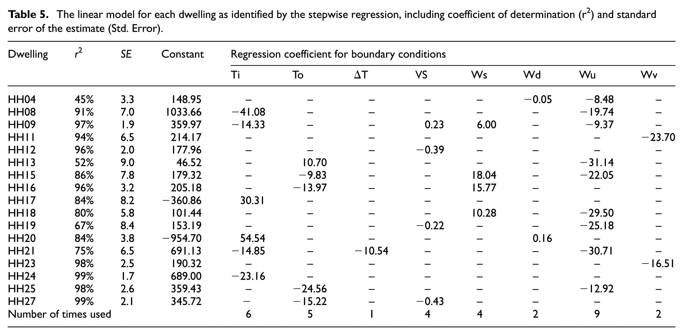
The linear models were able to explain most of the variability in the in-use HTC for the majority of dwellings: over 50% (r²>50%) of the variability for 16 of the 17 dwellings, and over 90% (r² > 90%) for 9 of those dwellings (Table 5). The coefficient of determination (r²) represents the proportion of the observed variability in the dependent variable which can be explained by using observed variability in the independent variables. The coefficient of determination across the 17 valid linear models varied from 45% to 99% with a mean of 85% (Table 5).

The standard error of the estimate (standard error) ranges between 1.7 W/ºC and 9.0 W/ºC, with a mean of 4.8 W/ºC. This represents the uncertainty in the model in predicting the average value of the dependent variable (HTC), demonstrating a close agreement between the measured and model-predicted values of the HTC.

Predicted in-use HTC for average aggregate heat loss test conditions

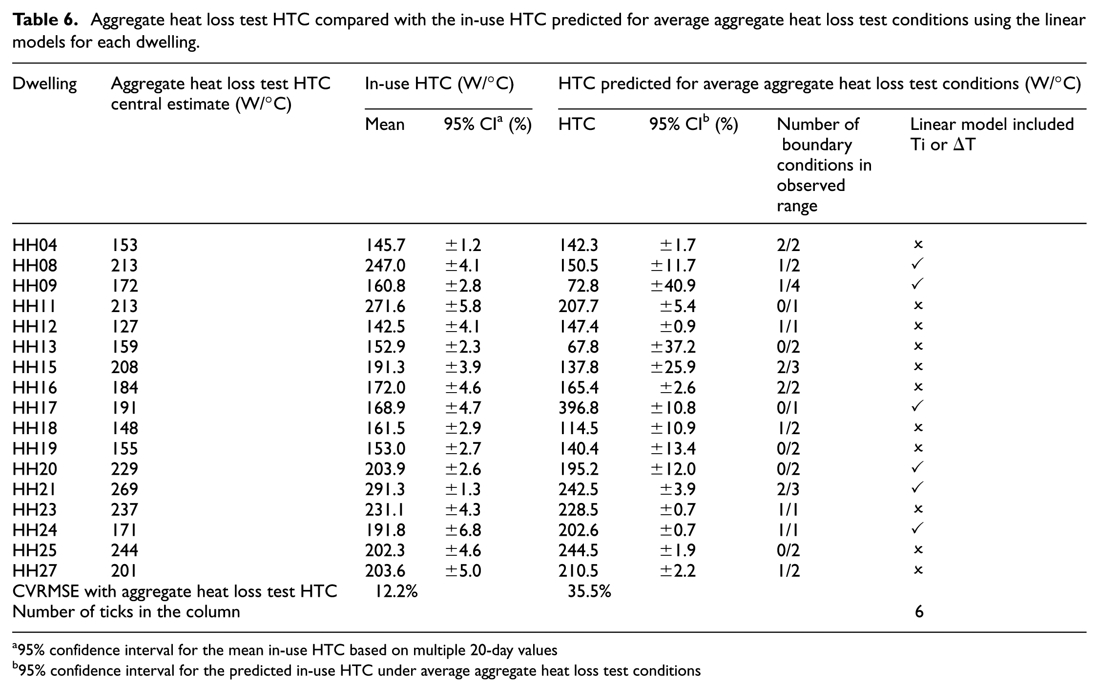
Predicting the in-use HTC for the average boundary conditions recorded during the aggregate heat loss test did not improve the comparison with the aggregate heat loss test HTC (Table 6, Figure 3). In fact, the agreement between the HTC predicted for average aggregate heat loss test conditions and the aggregate heat loss test results (CVRMSE = 35.5%) was worse than the in-use HTC compared with the aggregate heat loss test results (CVRMSE = 12.2%).

Table 6.

Aggregate heat loss test HTC compared with the in-use HTC predicted for average aggregate heat loss test conditions using the linear models for each dwelling.

Dwelling	Aggregate heat loss test HTCcentral estimate (W/ºC)	In-use HTC (W/ºC)		HTC predicted for average aggregate heat loss test conditions (W/ºC)
		Mean	95% CI^a (%)	HTC	95% CI^b (%)	Number of boundaryconditions inobservedrange	Linear model includedTi or ΔT
HH04	153	145.7	±1.2	142.3	±1.7	2/2	✕
HH08	213	247.0	±4.1	150.5	±11.7	1/2	✓
HH09	172	160.8	±2.8	72.8	±40.9	1/4	✓
HH11	213	271.6	±5.8	207.7	±5.4	0/1	✕
HH12	127	142.5	±4.1	147.4	±0.9	1/1	✕
HH13	159	152.9	±2.3	67.8	±37.2	0/2	✕
HH15	208	191.3	±3.9	137.8	±25.9	2/3	✕
HH16	184	172.0	±4.6	165.4	±2.6	2/2	✕
HH17	191	168.9	±4.7	396.8	±10.8	0/1	✓
HH18	148	161.5	±2.9	114.5	±10.9	1/2	✕
HH19	155	153.0	±2.7	140.4	±13.4	0/2	✕
HH20	229	203.9	±2.6	195.2	±12.0	0/2	✓
HH21	269	291.3	±1.3	242.5	±3.9	2/3	✓
HH23	237	231.1	±4.3	228.5	±0.7	1/1	✕
HH24	171	191.8	±6.8	202.6	±0.7	1/1	✓
HH25	244	202.3	±4.6	244.5	±1.9	0/2	✕
HH27	201	203.6	±5.0	210.5	±2.2	1/2	✕
CVRMSE with aggregate heat loss test HTC		12.2%		35.5%
Number of ticks in the column							6

95% confidence interval for the mean in-use HTC based on multiple 20-day values

95% confidence interval for the predicted in-use HTC under average aggregate heat loss test conditions

Figure 3.

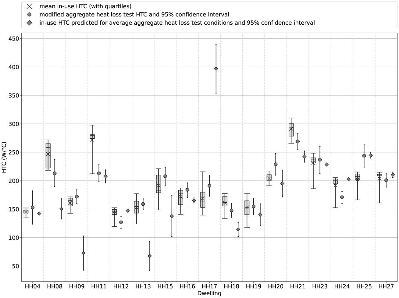
Box-whisker plots of the in-use HTC, aggregate heat loss test results with 95% confidence interval⁶ and the HTC predicted using average aggregate heat loss test conditions with 95% confidence interval for all dwellings in the sample.

The average aggregate heat loss test conditions were within the observed range for only four of the 17 models. It is hypothesised that the difference may be due to the extrapolation to an elevated indoor air temperature (average Ti was 20°C–25°C) as used during the aggregate heat loss test, with only six of the models having included Ti or ΔT: that is, the linear model could not account for changes in the indoor air temperature. This result demonstrates that the use of the linear model to extrapolate the results to boundary conditions outside of the observed range must be undertaken with caution.

Discussion

The results indicate that the variation in the in-use HTC of dwellings may be an important factor in the energy performance gap. The in-use HTC, calculated from 20-day rolling averages, had a COV between 1.0% and 11.8%, with an average of 7.1%. The monthly average SAP HTC, which is used for generating Energy Performance Certificates, had a COV of between 0.2% and 0.4%. Given that the HTC is varying, the period over which the HTC is averaged will affect the result. It is reasonable to expect that if the in-use HTC were calculated for single days over the heating season then the variation would be greater than if calculated for each month. Therefore, it is important to consider the averaging period alongside the variability when making any comparisons. Comparing the in-use HTC measured over a few days or weeks with a seasonal average in-use HTC could be misleading.

Accounting for the variability could improve the precision of in-use HTC by reducing the spread in the results. It was demonstrated in this paper that linear models could explain an average of 85% of the variability in the in-use HTC. The linear models can be used to account for differences in the average boundary conditions over different periods. This is an important benefit of longer-term monitoring of the in-use HTC, compared with short term measurement – monitoring in-use HTC over the year provide a direct measurement of the variability and the factors that can explain it.

The use of linear models to extrapolate the in-use HTC to boundary conditions outside of the observed range must be approached with caution. The use of the linear model to extrapolate the results to the average boundary conditions at the time of the aggregate heat loss test did not improve the predicted HTC, compared with the in-use HTC. It is hypothesised that this is because the aggregate heat loss test is usually carried out at elevated indoor air temperatures beyond those normally observed in an in-use dwelling. Previous research has questioned the applicability of the HTC derived by an aggregate heat loss test to the real-world thermal performance of an occupied dwelling, due to the elevated temperatures (Hollick et al., 2020). This finding suggests a need to develop new short-term test methods carried out at more typical indoor air temperatures, or ways to extend the range of boundary conditions when monitoring long term in-use conditions.

The SAP HTC model-based predictions fail to capture the variability in the in-use HTC. Each dwelling in this study had a unique linear model with different sets of predictor variables. Intuitively, the airtightness of a dwelling, its orientation and the degree of shelter from the wind will act together to impact how the rate of heat loss changes on windy days. Window size and orientation, as well as the time of year (which affects the sun path), are likely to impact on the response of a building to solar irradiance. U-values are a simplification of the real rate of heat loss through a building element and so the assumption that there are constant thermal resistances on the inside and outside surfaces neglects the temperature dependence of the convection and radiation heat transfer processes. People heat their homes in different ways, driving different indoor-outdoor temperature differences. It would be difficult to capture all of these variations in a building physics model. This finding highlights the need for in-use measurements to understand the real performance of dwellings. This will help develop better models and improve predictions.

More work is required to avoid any need for extrapolation of the in-use HTC. Standard boundary conditions could be developed, which allow the HTC of different dwellings to be directly compared, by interpolation. These could reflect the boundary conditions that most dwellings would experience over a normal winter and therefore represent the real average performance of the dwellings. For example, this could include the regional weather data in SAP version 10.2 (BRE, 2022) (accounting for the shelter factors applied in SAP) and the median indoor air temperature recorded during December 2017 to February 2018 as part of the national Energy Follow Up Survey using data from 750 English dwellings (HM Government, 2021b) (Table 7). Aggregate heat loss tests and QUB tests could be carried out at lower indoor air temperatures to aid comparison with interpolated in-use HTCs.

Table 7.

Possible standard boundary conditions for comparing the in-use HTC of different dwellings.

Standard boundary conditions for all dwellings
Ti (°C)^a	To (°C)^b	Δ T (°C)^c	VS(W/m²)^b	Ws(m/s)^b	Wd(°)^d	Wu(m/s)^c	Wv(m/s)^c
18.4	6.6	11.8	64.0	3.825	247.5	−1.464	−3.534

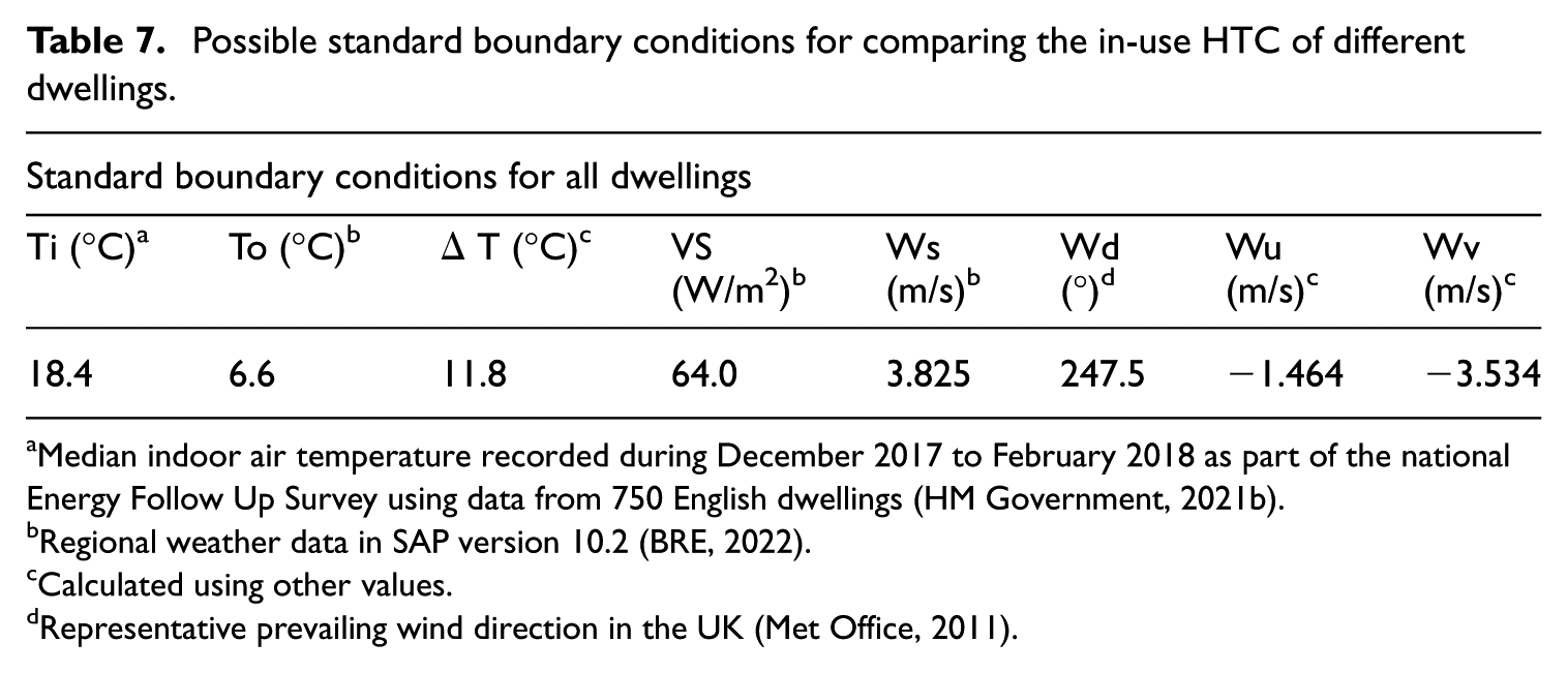
Median indoor air temperature recorded during December 2017 to February 2018 as part of the national Energy Follow Up Survey using data from 750 English dwellings (HM Government, 2021b).

Regional weather data in SAP version 10.2 (BRE, 2022).

Calculated using other values.

Representative prevailing wind direction in the UK (Met Office, 2011).

Despite using the largest publicly available dataset of its kind, this study was limited by the relatively short period of data collection over part of one winter, resulting in only 11–52 unique in-use HTC measurements for each dwelling. It is fully expected that longer periods of monitoring over a whole winter or winters will provide a wider range of boundary conditions for the linear models and therefore enable broader interpolation without the limitations of extrapolation beyond the observed data. Households could even be incentivised to heat their homes to higher temperatures if this would help with interpolating to certain temperature boundary conditions, such as those used in a QUB or aggregate heat loss test.

The impact of autocorrelation, due to overlapping 20-day periods, has not been assessed in this work. It is acknowledged that the proportion of variability which is explained by the linear models could change if the linear models are developed using non-overlapping 20-day periods. For the limited duration available in the dataset used in this work, it would not be possible to consider non-overlapping 20-day periods. However, this work presents a method of analysis which could be applied to longer datasets which allow for non-overlapping periods.

The work in this paper has not considered uncertainty in the measurement of the boundary conditions. Uncertainty in measured values of boundary conditions and energy demand can be expected to contribute to observed variation in the in-use HTC. If there was a relationship between a boundary condition and the uncertainty in its measurement, then uncertainty and variability would be conflated in any linear model relating the in-use HTC to the boundary conditions. It is assumed here that any measurement errors are independent of the boundary conditions, and that measurement uncertainty is therefore not conflated with variability.

This paper only considers the linear relationship between the in-use HTC and each boundary condition. It is possible that the influence of some boundary conditions might be better explained using a non-linear relationship. In some linear models, this could lead to the inclusion of some boundary conditions for which a linear relationship was not identified. One may expect this would improve the ability for models to accuracy explain the relationship between the HTC and the boundary conditions, and could be considered in future work. Transformations will be required to convert variables with a non-linear relationship with the HTC to ones with a linear relationship, such that they can be included in the stepwise regression method presented in this work.

This paper was only possible because of the development of methods to measure in-use HTC at scale, and the datasets that have resulted from their evaluation. More accurate SMETER methods are being developed and it is expected that the accuracy of in-use HTC measurements will improve even more rapidly when the variability is accounted for. Further work on a larger sample of dwellings which are monitored over longer periods of time is urgently needed to progress the development of in-use HTC measurement techniques. Future work might also consider the impact of other boundary conditions such as the temperature of the ground and the heat shared across party walls, previously treated as sources of uncertainty in HTC measurement in research to date, including that of IEA Annex 71 (Bauwens et al., 2021). The dwellings considered in this paper were typical of those in the UK housing stock. However, further research should consider dwellings with lower HTC values, including high performance dwellings and apartments.

The findings of this work are encouraging – it is possible to measure the in-use HTC in a way that accounts for variability caused by varying boundary conditions. The types of data generated when monitoring the indoor environment and energy demands of dwellings for calculating the in-use HTC will have wider applications to important matters such as monitoring fuel poverty, cold homes, indoor air quality, moisture and damp, and summertime overheating. Research and innovation in this space is expected to grow exponentially and it is hoped that this will support widespread adoption of in-use performance measurement.

Conclusion

This paper aimed to improve the precision of measurements of the in-use thermal performance of dwellings by explaining the variability in the in-use HTC caused by variations in the boundary conditions during different measurement periods. The in-use HTC of 19 dwellings was calculated over rolling 20-day periods for up to 6 months to quantify the magnitude of the variability. Linear models that explain the variability in the HTC as a function of the boundary conditions during the measurement were created.

The in-use HTC of the dwellings had a coefficient of variation (standard deviation divided by mean) of between 1.0% and 11.8%, with an average of 7.1%. This is the first time that the variability of HTCs has been quantified by measurement. This observed variability is much higher than that currently predicted by the RdSAP model used for generating Energy Performance Certificates (average coefficient of variation 0.3%) and therefore contributes to the energy performance gap. However, it is important to consider the averaging period alongside the variability when making any comparisons: comparing the in-use HTC measured over a few days or weeks with a seasonal average in-use HTC could be misleading.

The relationship between the in-use HTC and the boundary conditions at the time of the measurement varied between dwellings; consequently, unique linear models were required for each dwelling. The linear models were valid for 17 of the 19 dwellings. The linear models were able to explain at least 80% of the variability in 13 of 17 dwellings. However, the use of the linear model to extrapolate the in-use HTC to boundary conditions outside of the observed range must be approached with caution. Therefore, future work should focus on applying this method to longitudinal data collected from wider ranges of homes.

These findings highlight the benefits of longer-term monitoring of the in-use HTC, and the need to develop new short-term test methods, or ways to extend the range of boundary conditions when in-use monitoring. Further work to implement the widespread application of in-use measurements is needed to better understand the real performance of dwellings and improve predictions.

Footnotes

ORCID iDs

Max Eastwood

Ben M Roberts

Funding

The authors disclosed receipt of the following financial support for the research, authorship and/or publication of this article: This work was carried out as part of a research project pursued within the EPSRC and SFI Centre for Doctoral Training in Energy Resilience and the Built Environment (ERBE CDT). The EPSRC funding for the centre is gratefully acknowledged (grant EP/S021671/1).

Declaration of conflicting interests

The authors declared no potential conflicts of interest with respect to the research, authorship and/or publication of this article.

Notes

References

Acker

Alfred

Amos

, et al. (2023). GES DISC tutorials, 1 August. https://doi.org/10.5281/ZENODO.8361449

Allinson

Crawley

Elwell

, et al. (2024). Technical Evaluation of SMETER Technologies Project, Phase 2 data: Heat transfer coefficients, in-use temperature and energy data, local weather, dwelling information, and occupancy surveys from 30 English dwellings, 2019–2021. UK Data Service. https://doi.org/10.5255/UKDA-SN-856978

Allinson

Roberts

Lomas

, et al. (2022). Technical Evaluation of SMETER Technologies (TEST) Project. London: Department for Business, Energy and Industrial Strategy.

Allison

(1999) Multiple Regression: A Primer. Pine Forge Press.

Alzetto

Farmer

Fitton

, et al. (2018) Comparison of whole house heat loss test methods under controlled conditions in six distinct retrofit scenarios. Energy and Buildings 168: 35–41.

Bauwens

Ritosa

Roels

(2021) IEA EBC Annex 71 – Building energy performance assessment based on in-situ measurements: Physical parameter identification (report of Subtask 3) Belgium: KU Leuven. Available at: https://www.iea-ebc.org (accessed 29 September 2021)

Bauwens

Roels

(2014). Co-heating test: A state-of-the-art. Energy and Buildings 82: 163–172.

BEIS (2019) Appendix S: Reduced Data SAP for existing dwellings. The Government’s Standard Assessment Procedure for Energy Rating of Dwellings.

BEIS (2020a) Digest of United Kingdom Energy Statistics 2020. Available at: https://www.gov.uk/government/statistics/digest-of-uk-energy-statistics-dukes-2020 (accessed 8 March 2021)

10.

BEIS (2020b) Energy Consumption in the UK (ECUK) 1970 to 2019. National Statistics. Available at: https://www.gov.uk/government/collections/digest-of-uk-energy-statistics-dukes (accessed 25 February 2021)

11.

BRE (2020) Building energy performance assessment: Support website. Available at: https://www.ncm-pcdb.org.uk/sap/ (accessed 11 August 2022)

12.

BRE (2022) The government’s standard assessment procedure for energy rating of dwellings. Version 10.2. Available at: https://bregroup.com/sap/sap10 (accessed 27 June 2023)

13.

BSI (1981) BS 2846-2:1981 - Guide to Statistical interpretation of data - Part 2: Estimation of the mean: confidence interval. BSI.

14.

BSI (2017a) BS EN ISO 13370:2017: Thermal performance of buildings - Heat transfer via the ground - Calculation methods. BSI.

15.

BSI (2017b) BS EN ISO 13789:2017: Thermal performance of buildings — Transmission and ventilation heat transfer coefficients — Calculation method. BSI.

16.

BSI (2024) BS EN 17887-1:2024: Thermal performance of buildings. In situ testing of completed buildings. Data collection for aggregate heat loss test. BSI.

17.

George

Mallery

(2020) IBM SPSS statistics 26 step by step, 16th edn. Routledge.

18.

Gori

Johnston

Bouchié

, et al. (2023). Characterisation and analysis of uncertainties in building heat transfer estimates from co-heating tests. Energy and Buildings 295: 113265.

19.

HM Government (1996) The gas (calculation of thermal energy) regulations 1996 (SI 1996/439). UK Statutory Instruments. Available at: https://www.legislation.gov.uk/uksi/1996/439/regulation/2/made (accessed 15 May 2024)

20.

HM Government (2020) The Ten Point Plan for a Green Industrial Revolution. HM Government

21.

HM Government. (2021a) Approved Document L: Conservation of fuel and power. Volume 1: Dwellings. 2021 Edition. The Building Regulations 2010.

22.

HM Government (2021b) Energy Follow Up Survey: Thermal Comfort, Damp and Ventilation. HM Government

23.

HM Government (2021c). [Withdrawn] Green Homes Grant: make energy improvements to your home (closed), 19 July. Available at: https://www.gov.uk/guidance/apply-for-the-green-homes-grant-scheme (accessed 16 February 2024)

24.

HM Government (2022). Smart meter enabled thermal efficiency ratings (SMETER) technologies project: technical evaluation, 27 January. Available at: https://www.gov.uk/government/publications/smart-meter-enabled-thermal-efficiency-ratings-smeter-technologies-project-technical-evaluation (accessed 14 February 2024)

25.

Huta

(2014). When to Use Hierarchical Linear Modeling. The Quantitative Methods for Psychology, 10(1): 13–28.

26.

Hollick

Gori

Elwell

(2020) Thermal performance of occupied homes: A dynamic grey-box method accounting for solar gains. Energy and Buildings 208: 109669.

27.

IBM (2023a) Statistical significance - Cognos Analytics 12.0.0. Available at: https://www.ibm.com/docs/en/cognos-analytics/12.0.0?topic=terms-statistical-significance (accessed 31 August 2023)

28.

IBM (2023b) Stepwise Multinomial Logistic Regression - SPSS Statistics 29.0.0. Available at: https://www.ibm.com/docs/en/spss-statistics/29.0.0?topic=customers-stepwise-multinomial-logistic-regression (accessed 1 September 2023)

29.

IBM Corp (2023). IBM SPSS Statistics (29.0.2.0). IBM Corp.

30.

IEA (2023a) Building envelopes. Available at: https://www.iea.org/energy-system/buildings/building-envelopes (accessed 16 February 2024)

31.

IEA (2023b) Energy efficiency - Energy system. Available at: https://www.iea.org/energy-system/energy-efficiency-and-demand/energy-efficiency#tracking (accessed 16 February 2024)

32.

IEA (2023c). Heating, 11 July. Available at: https://www.iea.org/energy-system/buildings/heating (accessed 16 February 2024)

33.

IEA EBC (2024) IEA EBC - Annex 94 - Validation and Verification of In-Situ Building Energy Performance Measurement Techniques. IEA EBC.

34.

Jack

(2015). Building Diagnostics: Practical Measurement of the Fabric Thermal Performance of Houses. Loughborough University. Available at: https://hdl.handle.net/2134/19274 (accessed 21 October 2021)

35.

Johnston

Miles-Shenton

Farmer

(2015). Quantifying the domestic building fabric ‘performance gap.’ Building Services Engineering Research and Technology 36(5): 614–627.

36.

Johnston

Miles-Shenton

Farmer

, et al. (2013) Whole House Heat Loss Test Method (Coheating). Leeds: Leeds Beckett University

37.

Juricic

Goffart

Rouchier

, et al. (2021). Influence of natural weather variability on the thermal characterisation of a building envelope. Applied Energy 288: 116582.

38.

Juricic

Rabouille

Challansonnex

, et al. (2023) The Sereine test: Advances towards short and reproducible measurements of a whole building heat transfer coefficient. Energy and Buildings 299: 113585.

39.

Knief

Forstmeier

(2021) Violating the normality assumption may be the lesser of two evils. Behavior Research Methods 53(6): 2576–2590.

40.

(2022). Thermal Performance of UK Dwellings: Assessment of Methods for Quantifying Whole-Dwelling Heat Loss in Occupied Homes. Loughborough University.

41.

Marill

(2004) Advanced statistics: Linear regression, Part II: Multiple linear regression. Academic Emergency Medicine 11(1): 94–102.

42.

Marshall

Fitton

Swan

, et al. (2017) Domestic building fabric performance: Closing the gap between the in situ measured and modelled performance. Energy and Buildings 150: 307–317.

43.

Met Office (2011) Where are the windiest parts of the UK? Available at: https://www.metoffice.gov.uk/weather/learn-about/weather/types-of-weather/wind/windiest-place-in-uk (accessed 14 December 2023)

44.

Miles

Shevlin

(2001) Applying Regression & Correlation: A Guide for Students and Researchers. Sage.

45.

Mishra

Pandey

Singh

, et al. (2019) Descriptive statistics and normality tests for statistical data. Annals of Cardiac Anaesthesia 22(1): 67–72.

46.

Morris

(2013) Benchmarking Domestic Gas and Electricity Consumption to Aid Local Authority Carbon Reduction Policy. Loughborough University.

47.

Ofgem (2022) Energy Company Obligation (ECO). Available at: https://www.ofgem.gov.uk/environmental-and-social-schemes/energy-company-obligation-eco (accessed 16 February 2024)

48.

Ofgem (2023) Great British insulation scheme. Available at: https://www.ofgem.gov.uk/environmental-and-social-schemes/great-british-insulation-scheme (accessed 16 February 2024)

49.

Piddington

Nicol

Garrett

, et al. (2020) The Housing Stock of the United Kingdom. Watford: BRE Trust.

50.

Senave

Roels

Verbeke

, et al. (2019) Sensitivity of characterizing the heat loss coefficient through on-board monitoring: A case study analysis. Energies 12(17): 3322. https://doi.org/10.3390/en12173322

51.

Sougkakis

Meulemans

Wood

, et al. (2021) Field testing of the QUB method for assessing the thermal performance of dwellings: In situ measurements of the heat transfer coefficient of a circa 1950s detached house in UK. Energy and Buildings 230: 110540.

52.

Stamp

(2015) Assessing uncertainty in co-heating tests: Calibrating a whole building steady state heat loss measurement method. Available at: http://discovery.ucl.ac.uk/1478162/1/Stamp_2015_Thesis.pdf (accessed 12 November 2021)

53.

Thébault

Bouchié

(2018) Refinement of the ISABELE method regarding uncertainty quantification and thermal dynamics modelling. Energy and Buildings 178: 182–205.

54.

Wingfield

Bell

M-S

South

, et al. (2011) Evaluating the impact of an enhanced energy performance standard on load-bearing masonry domestic construction: Understanding the gap between designed and real performance: lessons from Stamford Brook. Available at: https://www.communities.gov.uk (accessed 20 May 2022)

55.

Zero Carbon Hub (2014) Closing the gap between design & as-built performance Evidence Review Report. Available at: https://www.zerocarbonhub.org (accessed 18 January 2021)

Measuring the in-use thermal performance of dwellings: improving the precision by accounting for variability

Abstract

Keywords

Introduction

Methods

Dataset

Calculating the HTC and its variability

Creating linear models to explain the variability in the in-use HTC

Predicting the in-use HTC for specific boundary conditions

Results

Variability in the HTC

Linear models to explain the variability

Predicted in-use HTC for average aggregate heat loss test conditions

Discussion

Conclusion

Footnotes

ORCID iDs

Funding

Declaration of conflicting interests

Notes

References