Sage Journals: Discover world-class research

Abstract

Meteorological mesoscale models with different urban parametrization are used to predict the local urban climate at 250 m resolution. The authors propose a hybrid machine learning approach to improve the mesoscale prediction accuracy using measured air temperature data from a sensor network and remove simulation bias. The simulation of the urban climate of Zurich during a hot summer is used as case study showing the improvements of the simulation accuracy. Based on the hybrid model results, a cumulative heat exposure index is proposed to map local hotspots in the city and assess the difference of cooling loads between rural and urban environments. Furthermore, intra-urban microclimatic differences of a typical mid-latitude city are explored to highlight the benefits of detailed simulations for building physics purposes.

Keywords

Machine learning mesoscale meteorological modeling urban climate intraurban analysis heat wave air temperatures heat exposure

Introduction

Due to the increasing magnitude and occurrence frequency of heatwaves (Easterling et al., 2000) and their important impact on buildings and urban environments, there is an urgent need for predicting the urban climate and local microclimates more accurately. During heatwaves, outdoor and indoor thermal comfort may deteriorate leading to excessive heat stress on pedestrians and inhabitants (Heaviside et al., 2017; Lass et al., 2011; Moonen et al., 2012; WHO Heatwaves, 2004). This negative impact may increase with climate change, for example rendering passive cooling by night ventilation ineffective and requiring the use of active cooling (Silva et al., 2022). Moreover, cities experience an urban heat island (UHI) effect, meaning they show higher temperatures compared to their rural surroundings. The UHI is caused by a variety of factors, such as the increase in sensible heat storage in building materials and roads exposed to solar radiation, the trapping of solar radiation in street canyons and in between buildings, the reduction in sky view factor and thus lower longwave radiative heat losses to the cold sky during nighttime, anthropogenic heat from waste heat due to building cooling and traffic, the reduction in evapotranspirative cooling due to a decrease in urban greenery and water bodies, and the reduction in urban ventilation and heat removal due to a reduction in wind speeds (Oke, 1982). Moreover, heatwaves become magnified by the UHI effect (McCarthy and Intergovernmental Panel on Climate Change, 2001; NASA, 2019b). In the review of Kong et al. (2021), the synergies between UHI and heatwaves are analyzed including a discussion of corresponding mitigation measures. A systematic literature review of mitigation measures for urban heatwaves with respect to geographical distribution, specific characteristics and pivotal actors is given by Hintz et al. (2018). In Zhao et al. (2023), a systematic decision-making methodology is presented for the selection of a set of mitigation measures at building and neighborhood scales, based on criteria like economic cost, effectiveness, and time for implementation.

Carmeliet and Derome (2024) discuss the use of physical modeling to understand the urban climate on scales down to individual buildings in order to develop adequate mitigation measures reducing urban heating. They distinguish three approaches at different scales to analyze the urban climate: climate-sensing, mesoscale meteorological models, simulating domain sizes between several hundred down to tens of kilometers, and urban microclimate models, simulating domain sizes from kilometers to tens of meters. An example of the first approach based on climate-sensing is the study of the UHI effect in five cities worldwide by Li et al. (2023) showing an upward trend over the last 30 years and spikes in cooling degree-hours for both urban and rural locations caused by climate change and urbanization. The second approach covers Mesoscale Meteorological Models (MMM), commonly used for weather prediction applications.

MMMs are downscaled using a down-nesting approach for urban climate simulation at grid resolutions between 2 km and 250 m. Down-nesting consists in feeding simulated data from a model at lower spatial resolution covering a large domain to a high-resolution model covering a smaller domain. MMMs are driven by lateral boundary and initial conditions from global circulation models. They model the time-dependent state of the atmosphere on a regular grid. Sub-grid scale physical mechanisms are represented by parametrized models. These parametrized processes usually include radiation, cloud physics, boundary layers, land use interaction but can also include urban climate effects. The effect of buildings on the urban climate is described by urban canopy parametrizations. Urban canopy models (UCM) solve the heat balance for a typical urban geometry, for example, a single or double street canyon (Schubert et al., 2012). The UCMs may be single- or multi-layered, where heat and momentum exchanges between urban surfaces are solved (Salamanca et al., 2011). Various building heights may be considered, and effects of shadowing, radiation trapping, and reflections are considered. Local turbulent air flow and buoyancy effects are not directly solved, but, for the convective heat exchange between air and building surfaces, convective transfer coefficients are used based on empirical correlations (Kusaka et al., 2001; Masson, 2000) or drag coefficients (Martilli et al., 2002). The use of UCMs requires the availability of detailed data describing the urban environment, like building geometry, land use data, and thermal properties of buildings. Commonly, the thermal and radiative properties are assumed to be uniform over the urban surfaces.

Mesoscale Meteorological Models can help to understand the causes of UHI and allow mapping the UHI over cities allocating local hot spots (Kong et al., 2023). MMM results have also been used by the authors as input to Building Energy Simulation (BES) tools to analyze summer overheating and excess building cooling demand during heatwave days and hot summers (Boudali Errebai et al., 2022). The authors compared WRF (Advanced Weather and Research Model) MMM predictions with weather station measurements and used the forecast data as input for the BES tool Energy+, finding that building cooling demand can be highly underpredicted during hot summers using standard reference meteorological data.

Despite all their capacities mentioned above, MMMs do not explicitly model all physical processes at play in a built environment and give only smeared evaluations of the impact of mitigation measures on UHI. Therefore, urban microclimate models need to be used for the analysis of the urban climate at local scale and for the design of adequate mitigation measures. These models explicitly model the physical processes involved, like turbulent air flow due to wind and buoyancy, shortwave solar radiation and longwave radiative exchanges between buildings and sky, heat and moisture transport processes in the air and porous material domains and use commonly Computational Fluid Dynamics (CFD). Vegetation is modeled as a porous medium including transpirative cooling, shadowing, and drag force (Manickathan et al., 2018). These models may provide information on local variables, such as air temperature, mean radiant temperature (the equivalent temperature considering all radiative exchanges to which a person is exposed), relative humidity, and air speed, necessary for thermal comfort analysis.

Toparlar et al. (2017) provide an extensive review on the use of CFD in urban microclimate analysis showing that there is a growing interest in the study of urban mitigation measures and linking the results from urban microclimate analysis with building related aspects, such as building energy consumption and indoor air temperature. Moonen et al. (2012) give an overview on the use of CFD in urban physics for analysis of wind comfort, wind-driven rain and thermal comfort, and discuss the impact of the microclimate on building energy demand. Despite the growing popularity of urban microclimate CFD modeling, Mirzaei (2021) remarks that such approaches still display main limitations such as the huge amount of needed computational resources, the need for better integration of urban climate CFD models and available data in cities, simplifications in defining adequate boundary conditions such as isothermal assumption of buildings (uniform building surface temperature), neglect of anthropogenic heat sources or steady state assumption of urban climate, and simplifications inherent to the use of turbulence models like in Reynolds-averaged Navier-Stokes equations.

Recently, Kubilay et al. (2020) coupled MMMs with CFD urban microclimate model solved using OpenFoam (Kubilay and OpenFOAM Community, 2024). In this one-way coupling approach between mesoscale and microscale, boundary conditions from MMMs are used to drive the urban microclimate model by interpolating wind and temperature profiles at the boundaries of the CFD domain.

From the above emerges a need for accurate simulations of the urban microclimate, especially during summer or heatwaves. Predictions by MMMs can be used as adequate environmental boundary conditions for such building and urban physics studies taking into account the local urban climate. In this paper, we first present the heat exposure index as a metric to analyze the severity of heatwaves and UHI based on measurement at urban and rural locations. This analysis allows selecting certain heatwaves to be reanalyzed using MMM. Then, we present a new approach to increase the prediction accuracy for urban climate simulations using MMM based on a hybrid workflow, where the results of MMM simulation are improved with machine learning (ML) based on measurement data.

The paper is organized as follows. In Section “Heatwave analysis over the last 30 years in Zurich,” we present an analysis of the heatwaves over the last 30 years in Zurich allowing to select a heatwave for further reanalysis. In Section “Mesoscale Meteorological Modeling (MMM) of a summer urban climate in Zurich,” we present two mesoscale meteorological models, compare their results with measured data from three weather stations and propose an improvement of the models using machine learning. In section “Urban heat island and intra-urban climate analysis,” we analyze the urban heat island of Zurich based on the MMM results toward an intra-urban microclimatic exploration using the heat exposure index. Finally, we finish with conclusions and outlook for future research.

Heatwave analysis over the last 30 years in Zurich

For testing out our new method, we chose the City of Zurich as the implementation location. Zurich is a mid-latitude city in Central Europe. It is classified as Cfb (Temperate Oceanic Climate) according to the Köppen-Geiger climate classification (Beck et al., 2018). The population of the municipality is around 440,000 (Statistik Zurich, 2023) and the total urban area counts 1,415,000 inhabitants. The population density is 5034 pers./km² (Federal Office of Statistics, 2022). Zurich is situated in a quite diverse topographical setting (see Figure 3(b)). The lake of Zurich and the surrounding hills determine the shape of the city. Roughly, one can differentiate between two parts of the city. The central, and main, part is situated near the lake and along the Limmat river flowing north. The northern neighborhoods Oerlikon, Schwamendingen, Affoltern, and Seebach located in the Glatt valley form the second part. The highest elevation is at 869.9 m and the lowest at 391.2 m height above mean sea level.

Recent overviews of different definitions for heatwaves are given in Kong et al. (2021) and Xu et al. (2020). Usually, a heatwave is defined as a consecutive period of a given minimum number of days, often three, with meteorological variables exceeding certain thresholds. These variables can be maximum air temperature, mean air temperature, mean radiant temperature, relative humidity, or indices based on a combination of these variables, like the Universal Thermal Climate Index (UTCI) or the Physiological Equivalent Temperature (PET). The thresholds of these parameters are dependent on the background climate. The most recent official Swiss definition is based on the mean air temperature over a certain period of time with a significant increase in mortality (Ragettli et al., 2023). In this paper, we use a simple heatwave definition, that is, the occurrence of minimal three consecutive days with a maximum air temperature equal or above 30°C.

Despite being situated in a temperate climate, Zurich experienced 37 heatwaves according to our definition, over the period of available data from 1994 until 2023. The urban heat island intensity (UHII), which is the difference in air temperature between the urban and rural station, over the whole period ranges from 5°C up to 9°C. The average UHII for all heatwaves is 2.5°C. In Figure 1, the heatwaves that occurred between 2017 and 2022 in Zurich and their associated UHII are plotted. The blue line shows the measured temperature at Zurich airport, considered rural, the red line at Kaserne in the center of Zurich, considered urban, while UHII, is shaded in light red and plotted with a black line. Each year since 2017 contains at least one heatwave. The heatwaves are of different maximum intensity, with an UHII ranging from 5.1°C to 7.7°C, and durations ranging from 3 to 11 days.

Figure 1.

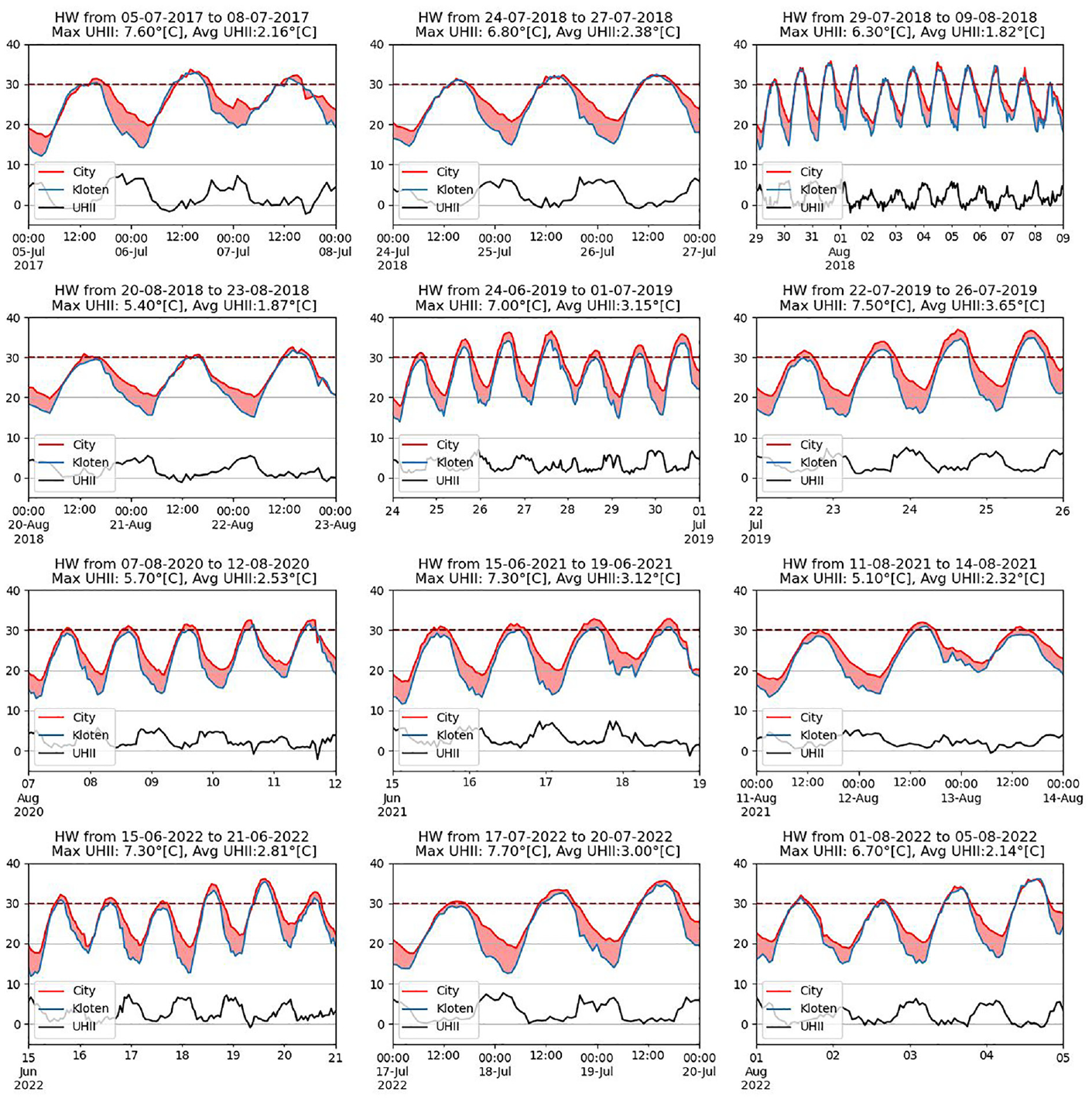
Air temperature at rural and urban stations, and Urban Heat Island Intensity (UHII) of the heatwave events in Zurich from 2017 until 2022. UHII is measured as difference between the urban station (City, NABEL Kaserne, Altitude: 505 m) and the rural station (Kloten, MeteoSwiss Zurich Airport, Altitude: 426 m).

To further analyze the summer climatic conditions in Zurich, we use a cumulative heat exposure index, similar to the ones used in Hondula et al. (2021) and Kong et al. (2023). The heat exposure index (HEI) for a certain threshold temperature is defined as:

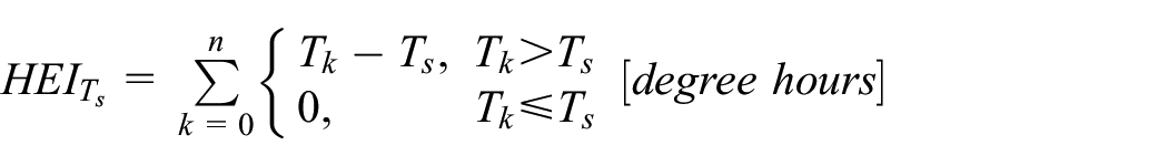
{H E I}_{T_{s}} = \sum_{k = 0}^{n} {\begin{matrix} T_{k} - T_{s}, & T_{k} > T_{s} \\ 0, & T_{k} \leq T_{s} \end{matrix} [d e g r e e h o u r s]

where T_s denotes the threshold temperature, k the index of summation, n the total hours in the considered period, and T_k the air temperature at 2 m height. The use of the HEI has several advantages over other thermal comfort indices: it is a cumulative quantity, so effects of heat can be considered over different intervals, for example, during heatwave days, monthly or yearly, to characterize the severity of heat exposure. It can be easily calculated, works equally well for simulations and measurements and can be plotted spatially to detect hot spots in a city. Although other variables could be chosen, such as the UTCI, but the air temperature is more easily accessible from both meteorological measurements and simulations.

We calculate the HEI using the measurements between 1991 and 2023 at both urban and rural stations in Zurich. We aggregate the results to yearly sums to examine the change in heat exposure over several years. The results of yearly HEI with a threshold temperature of 26°C are plotted in Figure 2. This value reflects a thermal comfort threshold and is used as threshold in the UTCI (Bröde et al., 2012), but other values can be used as can be found in the Appendix A5 for a threshold value of 23°C. The results in Figure 2 show a high scatter with values ranging from 150 to 2451 degree-hours (dh), according to the occurrence of hotter and cooler years. Especially the year 2003 is found to be an extremely hot year (2451 dh in the urban and 1819 dh in the rural area), remembered for an excessive heatwave over Europe, followed by the years 2015 (1968/1484 dh) and 2022 (1873/1262.2 dh). If we fit an ordinary least square (OLS) model to the time series, we can see an increasing trend in HEI both in the rural and urban areas. However, the fitted line is steeper in the urban area. The change of heat exposure with a threshold temperature of 26°C between 1991 and 2023 is 61% (537 dh/year) at the rural station and 68% (927 dh/year) at the urban station.

Figure 2.

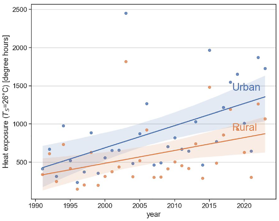
Heat exposure with threshold temperature of 26°C for the urban (City NABEL Kaserne) and rural (Kloten, MeteoSwiss Zurich Airport) stations from 1991 to 2023.

In the next section, we simulate the urban climate from June 1st until July 31st, 2019. The year 2019 is the fifth hottest year during the period 1991–2023. This period includes two heatwaves, where the first shows an urban HEI of 527 dh, which is the fifth severe heatwave, while the second heatwave shows an urban HEI of 316 dh, which is the eighth severe heatwave during the period 1991–2023. Note that the complete period between June 1st and July 31st, 2019, includes also colder days with average or below average temperatures.

Mesoscale Meteorological Modeling (MMM) of a summer urban climate in Zurich

Description of the Mesoscale Meteorological Models (MMM)

MMMs, such as WRF (Advanced Weather and Research Model; Skamarock et al., 2019) and COSMO (Consortium for Small-scale Modelling; Doms and Baldauf, 2011), commonly used for weather prediction (Orlanski, 1975), can also be configured to study the urban climate at 250 m resolution. The methods are based on a down-nesting of initial and boundary conditions obtained from global models like GFS (global forecast system), ECMWF (European Centre for Medium-Range Weather Forecasts), or from nested models derived from the global ones like MeteoSwiss COSMO-2/1. At the boundaries of the spatial domain, lateral boundary conditions are prescribed which come from the results at higher scale and a relaxation zone is implemented to blend the forced conditions at the boundaries together with the atmospheric model of a limited area (Davies, 1976). Figure 3(a) shows our down-nesting approach for the WRF model at three steps for the city of Zurich, where the largest domain D01 has a grid size of 6.25 km and the smallest domain D03, which is the domain of interest, a grid size of 250 m. The largest domain measures 812.5 × 806.25 km², the domain D02 182.5 × 176.25 km², and domain D03 50.25 × 50.25 km². Figure 3(b) shows Zurich and its surroundings, and the locations of the ground truth sensors that will be used in our hybrid ML model in Section “Improved WRF model using machine learning (ML).” Ground truth sensors provide the true temperature of the environment for fitting the ML model.

Figure 3.

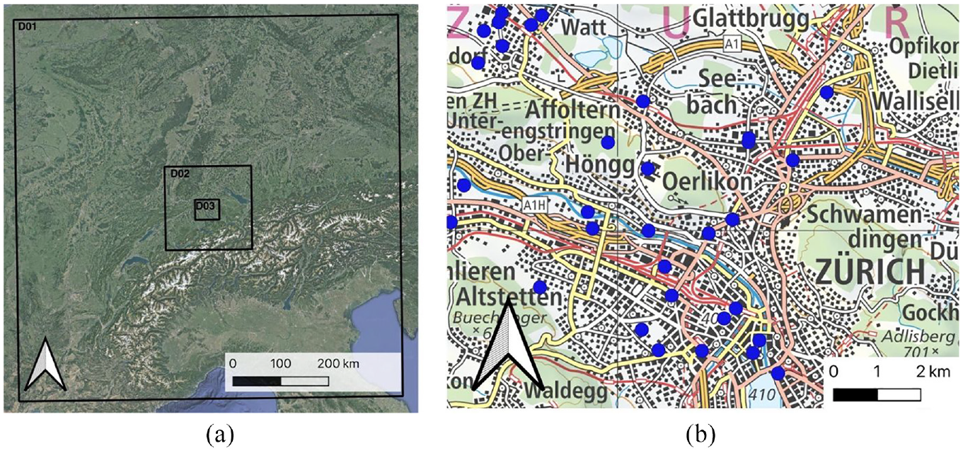
(a) Setup of the nested domains for WRF simulation of Zurich with three domains D01, D02, and D03. Map data ©2019 Google. (b) Locations of the ground truth sensors in Zurich and its surroundings. Map data: Swisstopo Landeskarte 1:25000 (2023).

For this paper, the authors have run several MMM simulations. For the comparison of WRF and COSMO, we have run the two models from June 10th 2019 until July 10th 2019. For fitting the ML model, we have used a WRF simulation run from the core summer season from June 1st to July 31st 2019. For the intraurban analysis, we have used a full WRF summer season run from June 1st until September 30th 2019.

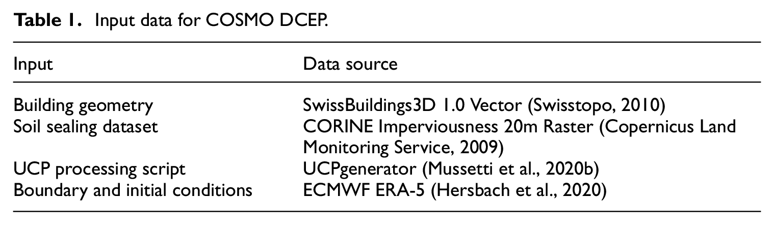
Several physical processes occurring at urban scale cannot be modeled directly in MMMs at the scale of 250 m and are represented by parametrized models. In COSMO, we use a urban canopy parametrization, named the double-canyon effect parametrization (DCEP) model (Schubert et al., 2012) for multi-layer urban canopy representation. A schematic drawing of DCEP is shown in Figure 4(a). DCEP is a multilevel urban canyon parametrization, using predefined height levels as refinement of the standard model levels in COSMO. This model takes into account the radiation exchange for two neighboring canyons, treating direct and diffuse radiation separately. Building morphology in each 250 × 250 m² area is grouped in four categories with different street orientation, building height, and street width. The use of DCEP needs a detailed preparation of input data such as building geometry, and radiative and thermal properties of urban surfaces, which can be processed from available LIDAR measurements or building databases. The data sources used in the present study are listed in Table 1. Mussetti et al. (2020b) developed a script called UCPGenerator for transforming these inputs into cell fractions for DCEP. Figure 4(b) shows as examples, the urban area fraction ranging from zero to one according to the soil sealing dataset and the fraction of buildings with a height of less than 20 m. Additional quantities calculated are the average width of streets and buildings in the domain.

Figure 4.

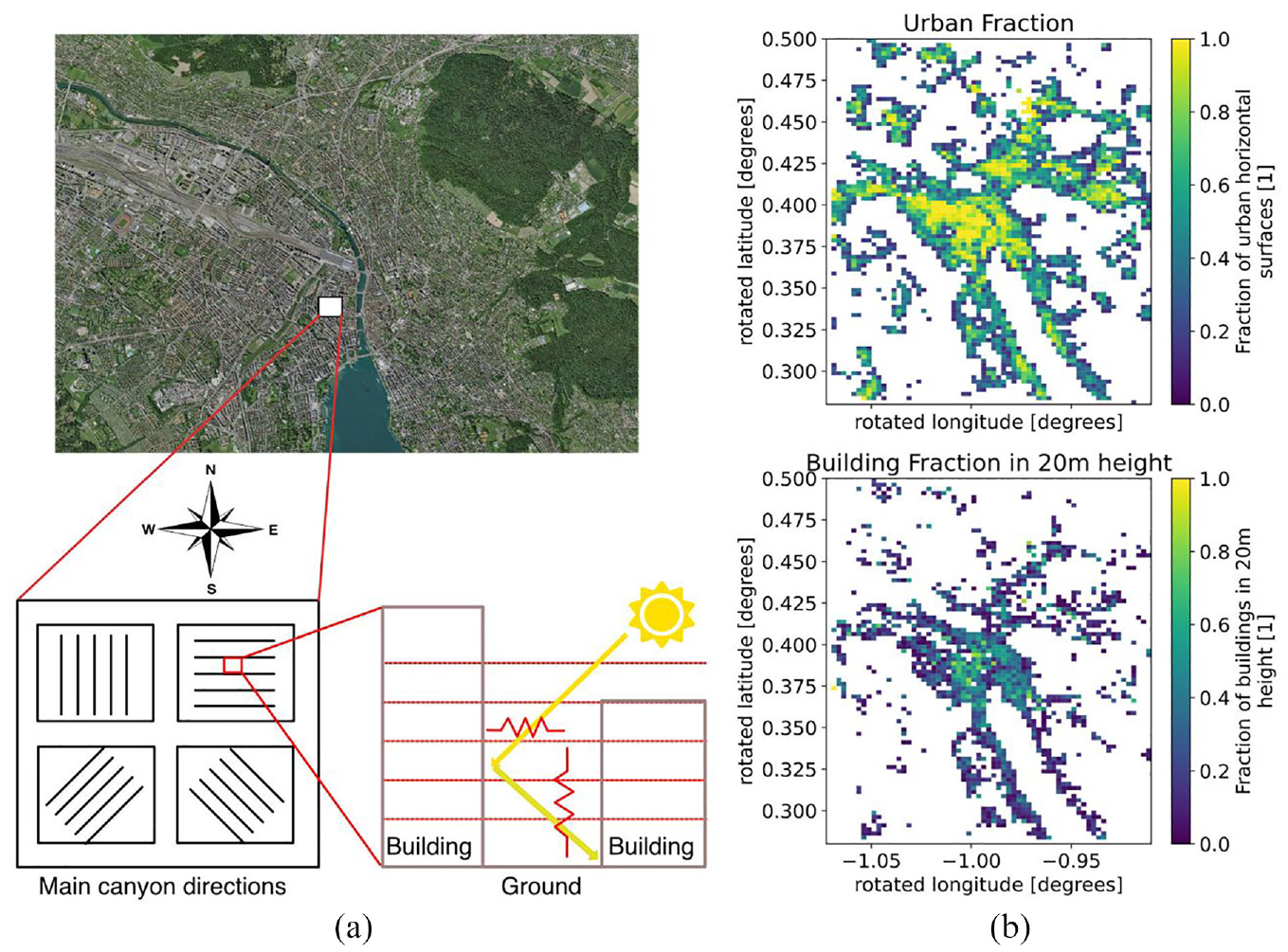
(a) Schematic description of DCEP urban parametrization model. (b) Spatial map of urban area fraction and the fraction of buildings lower than 20 m for Zurich.

Table 1.

Input data for COSMO DCEP.

Input	Data source
Building geometry	SwissBuildings3D 1.0 Vector (Swisstopo, 2010)
Soil sealing dataset	CORINE Imperviousness 20m Raster (Copernicus Land Monitoring Service, 2009)
UCP processing script	UCPgenerator (Mussetti et al., 2020b)
Boundary and initial conditions	ECMWF ERA-5 (Hersbach et al., 2020)

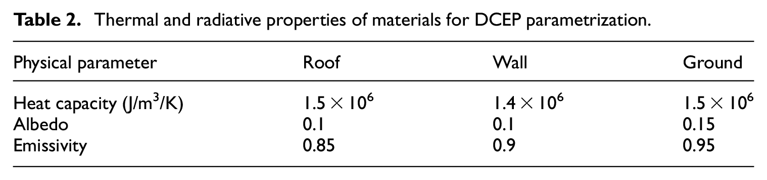
For running the model, physical properties have to be assigned to roofs, ground, and walls. The thermal and radiative properties of in DCEP are listed in Table 2. These values are used uniformly over the whole city for all street canyons. Using uniform values for these properties is a significant simplification, since the urban environment is much more complex, showing different building stock and varying surface types. However, detailed information about the thermal and radiative properties of these components is not directly available.

Table 2.

Thermal and radiative properties of materials for DCEP parametrization.

Physical parameter	Roof	Wall	Ground
Heat capacity (J/m³/K)	1.5 × 10⁶	1.4 × 10⁶	1.5 × 10⁶
Albedo	0.1	0.1	0.15
Emissivity	0.85	0.9	0.95

In the present study, COSMO-DCEP simulations are performed with a timestep of 5 s and with hourly output of results. Mussetti et al. (2020a) studied the performance of this approach for Zurich and showed that using a higher resolution of 250 m compared to a commonly-used resolution of 1 km improved the prediction of the urban climate.

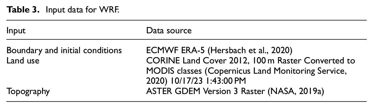
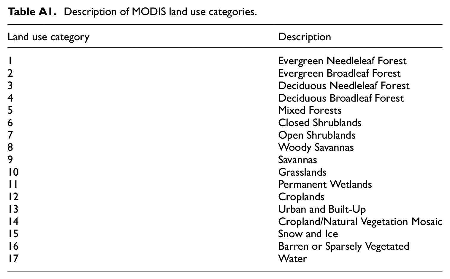
In our WRF simulations, we use the NOAH Land Surface Model (LSM) to model the exchange of heat and moisture between soil and the atmosphere. The NOAH scheme is widely used in operational weather forecasting and is considered to be one of the default LSM schemes in WRF. It was developed through an interdisciplinary research project, grouping several universities and US governmental agencies, and continues to be improved by WRF developers. The LSM scheme plays a critical role in predicting surface and near-surface variables like air temperature at 2 m, surface temperature, wind speed, and energy fluxes between the atmosphere and the ground. In our WRF setup, we use the NOAH LSM for the urban environment without any additional urban canopy models. All used input data is listed in Table 3. A detailed description of all WRF variables can be found in the WRF User’s Guide (WRF User’s Guide, 2020) and is given in Appendix A1. A map and description of the land use categories is given in Appendix A2 (Figure A1). The WRF and COSMO simulations are carried out over two summer months from June 1st until July 31st, 2019.

Table 3.

Input data for WRF.

Input	Data source
Boundary and initial conditions	ECMWF ERA-5 (Hersbach et al., 2020)
Land use	CORINE Land Cover 2012, 100 m Raster Converted to MODIS classes (Copernicus Land Monitoring Service, 2020) 10/17/23 1:43:00 PM
Topography	ASTER GDEM Version 3 Raster (NASA, 2019a)

We finally remark that the effort in preparing the input for WRF-NOAH is much less labor-intensive in comparison to the COSMO-DCEP.

Validation of the COSMO-DCEP and WRF-NOAH MMM models

The two models are validated with weather station data from MeteoSwiss and NABEL (National Air Pollution Monitoring Network). Figure 5(a) shows the locations of three measurement stations in Zurich used for comparison with the results of WRF and COSMO. Each of these three stations is located in a different environment type. Kaserne station is situated in the city center of Zurich, representing an urban area, and is part of the national NABEL pollution measurement network. The station measures, apart from pollution parameters, the whole set of standard meteorological parameters. The temperature measurement is performed with Thygan VTP 6, a ventilated and shaded thermo-hygrometer, approved by the World Meteorological Organization (WMO). Measurements are carried out according to the WMO standards at 2 m height (Fischer, 2023). The station is situated on an open space in a big courtyard which should minimize the effects of nearby buildings. We use only the air temperature for validation, and not the other data like wind which shows much higher fluctuations. SMA station is located on a hill facing south-west around 170 m above the city center and represents a semi-urban area. The airport station is situated just outside the city and is considered semi-rural. These two stations are part of the MeteoSwiss national station network and measure all parameters according to the WMO standards. We assess the NABEL and MeteoSwiss measurements suitable for validation purposes and use only the data from these three stations for validation. We use the sensor dataset installed over Zurich and rural surrounding area for the improvement of the WRF model using Machine Learning (ML), as explained in Section “Improved WRF model using machine learning (ML).”

Figure 5.

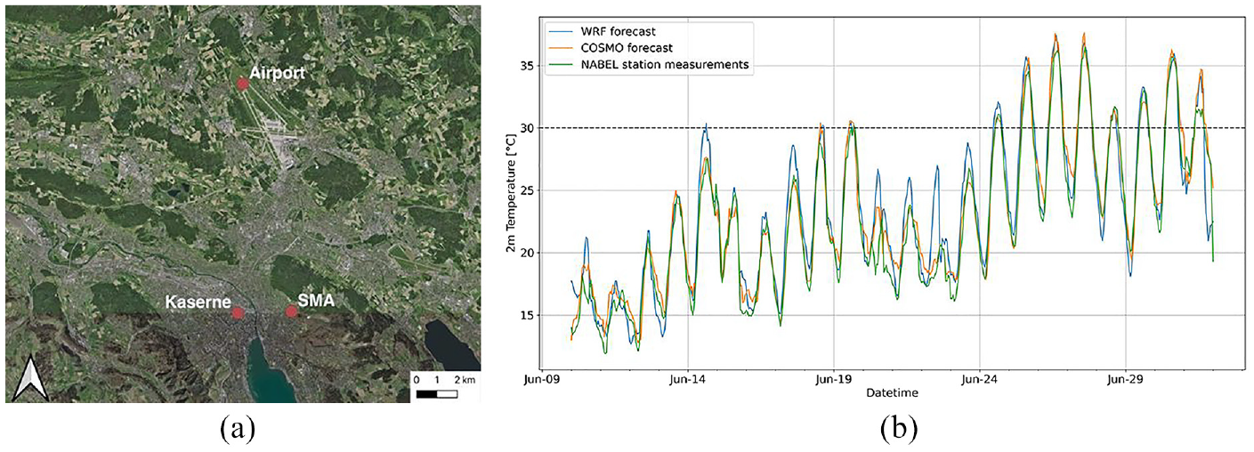
(a) Locations of selected measurement stations in Zurich area for validation purposes. (b) Comparison of air temperature at 2 m height between WRF, COSMO, and measured data from the meteorological measurement station in central Zurich (NABEL) during a summer period from June 10th 2019 until July 10th 2019 including one heatwave. The dashed line at 30°C indicates the threshold for heatwaves retained in our study.

Figure 5(b) compares the predictions of air temperature from the closest COSMO and WRF cells at 2 m height above ground (T2m) with the measured data at the urban station Kaserne at the same height for the heatwave during June 2019. WRF overpredicts daily peaks especially between June 20th and June 23rd but also on June 15th and June 18th. Although COSMO predicts the daily peaks better than WRF, its predictsions are too warm for the nights, for example from June 20th until June 23rd and on June 26th and 27th. Table 4 shows the RMSE (Root Mean Square Error) values for the three stations over the whole period from June 10th to July 10th, 2019. The RMSE is defined in Appendix A4. The RMSE values are mainly between 1°C and 2°C, and not larger than 3°C.

Table 4.

RMSE values for COSMO and WRF predictions from June 10th to July 10th, 2019, at the locations of the three measurement stations.

Reference station	COSMO	WRF
Kaserne (urban)	1.26°C	1.87°C
SMA Fluntern (semi-urban)	1.82°C	2.76°C
Airport (semi-rural)	1.57°C	2.8°C

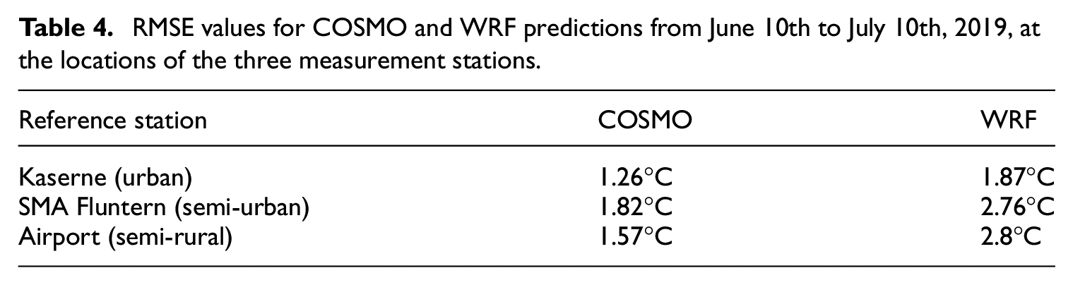
COSMO with the computationally and labor intensive urban canopy parametrization performs better than WRF. However, WRF with the default NOAH land use modeling is not much worse especially in the urban environment like the one at Kaserne station. The discrepancy between the two models can be attributed to different reasons. First, we note that the measurements at the weather stations may be strongly influenced by the local situation around the stations, and is representative only locally, while in the simulations the air temperature is the mean value averaged over the cell measuring 250 × 250 m². Second, a validation based on only three measurement locations is limited, which is due to a shortage of meteorological stations in the urban area of Zurich. This leads to a heavy bias in the validation since the spatial model is not properly evaluated. However, this is the best reference data available for the domain and the results warrant improvement of MMM simulation results. In the next section, we present a hybrid method based on Machine Learning (ML) to improve the agreement between simulation and observation data for the air temperature at 2 m (T2m).

Improved WRF model using machine learning (ML)

We apply a machine learning method (ML) to improve the WRF predictions in the domain of interest D03. The results of WRF simulation (referred to as WRF-only) are corrected for the bias between simulation and measured data with a machine learning approach (referred to as WRF + ML). In Zurich, a dense network of microclimate stations has been built in the last 3 years to provide diverse ground truth data over the whole city. Figure 3(b) shows the spatial distribution of temperature sensors over Zurich and its surrounding environment. The sensors are manufactured by the company Decentlab, are shielded against radiation and are based on the standard sensor SHT35 by the company Sensirion. These sensors are factory-calibrated with an accuracy of ±1.5% RH and ±0.1°C (Baum and Sintermann, 2021; Sensirion, 2022). The sensor network for 2019 contains 40 devices communicating their data by LoRaWAN at 10-min intervals. They are mounted on streetlamp posts at 2 m height. There is also a sensor network in the rural environment of the Canton of Zurich (Baum and Sintermann, 2021). These stations measure the air temperature of the local environment, which is also the target variable for the machine learning model.

Different ML algorithms were tested, such as Support Vector Machine, Neural Network, and Gradient Boosted Trees. It was found that the best RMSE performance is provided using a random forest approach. Data from all stations are used for training the model. All dynamic and static variables of the WRF output are also included as predictors and listed in Appendix A1. The assembled dataset is split in 70% training and 30% validation data. A random shuffling of both batches is applied to reduce the influence of temporal patterns and the chances of overfitting. The mean decrease of impunity (MDI), or Gini importance, of the input variables has been calculated for evaluating the importance of each input variable (see Appendix A3). Figure A2 in the appendix shows that the most significant variables are T2 (Temperature at 2 m, feature importance: 0.77), followed by GRDFLX (Ground heat flux, feature importance: 0.049), TH2 (Potential Temperature at 2 m, feature importance: 0.014), and MU (perturbation dry air mass in column, feature importance 0.007).

Additional static data like topography, land classification according to cadaster and exposition are initially also included in the analysis. We found that the additional static data do not increase or even decrease the prediction accuracy. A possible explanation is that the static data are already included as input in the WRF simulation itself, that is, WRF already uses static datasets, like topography and land use data, for boundary layer, surface, and soil parametrization. Hence, including this data into the ML process does not introduce new information.

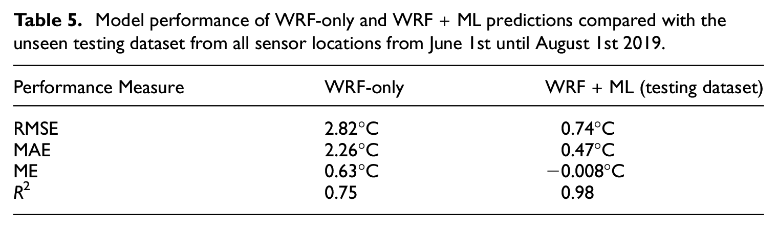
Table 5 shows the model performance measures (defined in Appendix A4) for the predictions of WRF-only and WRF + ML against the unseen testing dataset from all sensor locations. A remarkable improvement of the accuracy of the predictions is observed showing a decrease of RMSE from 2.82°C for WRF to 0.74°C for WRF + ML. The MAE (Mean Absolute Error) is close to the RMSE values which indicates the results are not dominated by outliers in the model. The ME (Mean Error) shows the overall bias of the model. A positive value indicates the model is predicting too high temperatures, negative values indicate that predicted temperatures of the model are too low. Without our hybrid ML approach, WRF temperatures are overall too high. This bias can be eliminated by applying our proposed hybrid model leading to a very minor bias of −0.008°C.

Table 5.

Model performance of WRF-only and WRF + ML predictions compared with the unseen testing dataset from all sensor locations from June 1st until August 1st 2019.

Performance Measure	WRF-only	WRF + ML (testing dataset)
RMSE	2.82°C	0.74°C
MAE	2.26°C	0.47°C
ME	0.63°C	−0.008°C
R ²	0.75	0.98

To investigate the model performance of the WRF + ML in more detail, we define three characteristic periods during our simulation period: non-heatwave, pre-heatwave and heatwave periods, and compare the predictions for these periods with the air temperature measured at 2 m at Zurich Kaserne weather station. Figure 6 shows the measured air temperature over the whole simulation period highlighting characteristic periods, representing non-heatwave, pre-heatwave and heatwave. Additionally, we define nighttime (22:00–06:00) and daytime (06:00–22:00) subphases during these three periods.

Figure 6.

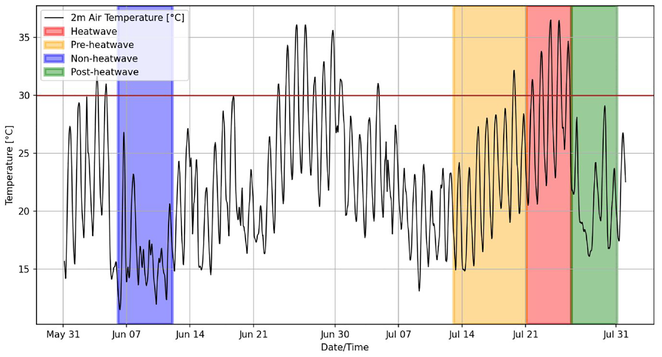
Measured 2 m air temperature at Zurich Kaserne station (NABEL) during the simulation period. Marked in red is a heatwave period, in orange a pre-heatwave, in green a post-heatwave, and in blue a non-heatwave period.

Table 6 shows RMSE, R², MAE, and ME values for the different selected periods and time frames. In general, in terms of RMSE, the model performs the best in the pre- heatwave period for nighttime hours and for all-day. The highest RMSE value is obtained during the heatwave day, but the difference between the highest and lowest RMSE is smaller than 0.16°C. Other performance measures are very close like model bias and MAE or identical like R². Overall, the best agreement is obtained for the non-heatwave period with all hours of the days selected: RMSE is 0.03°C higher, R² lower at 0.966 and MAE is lower at 0.441°C compared to the other periods. Model bias is in the opposite direction showing a prediction of slightly higher temperatures.

Table 6.

Model performance during non-heatwave, pre-heatwave and heatwave periods for all-day, daytime (06:00–22:00) and nighttime (22:00–06:00).

Selected Period	RMSE (°C)	R ²	MAE (°C)	ME (°C)
Non-heatwave all-day	0.707	0.966	0.441	0.014°C
Before-heatwave all-day	0.668	0.982	0.453	−0.007°C
Heatwave all-day	0.782	0.980	0.512	−0.014°C
Non-heatwave day	0.803	0.960	0.513	−0.019
Before-heatwave day	0.708	0.978	0.480	−0.045
Heatwave day	0.827	0.977	0.537	−0.108
Heatwave night	0.784	0.980	0.512	−0.022
Non-heatwave night	0.714	0.966	0.446	0.013
Before-heatwave night	0.672	0.982	0.455	−0.006

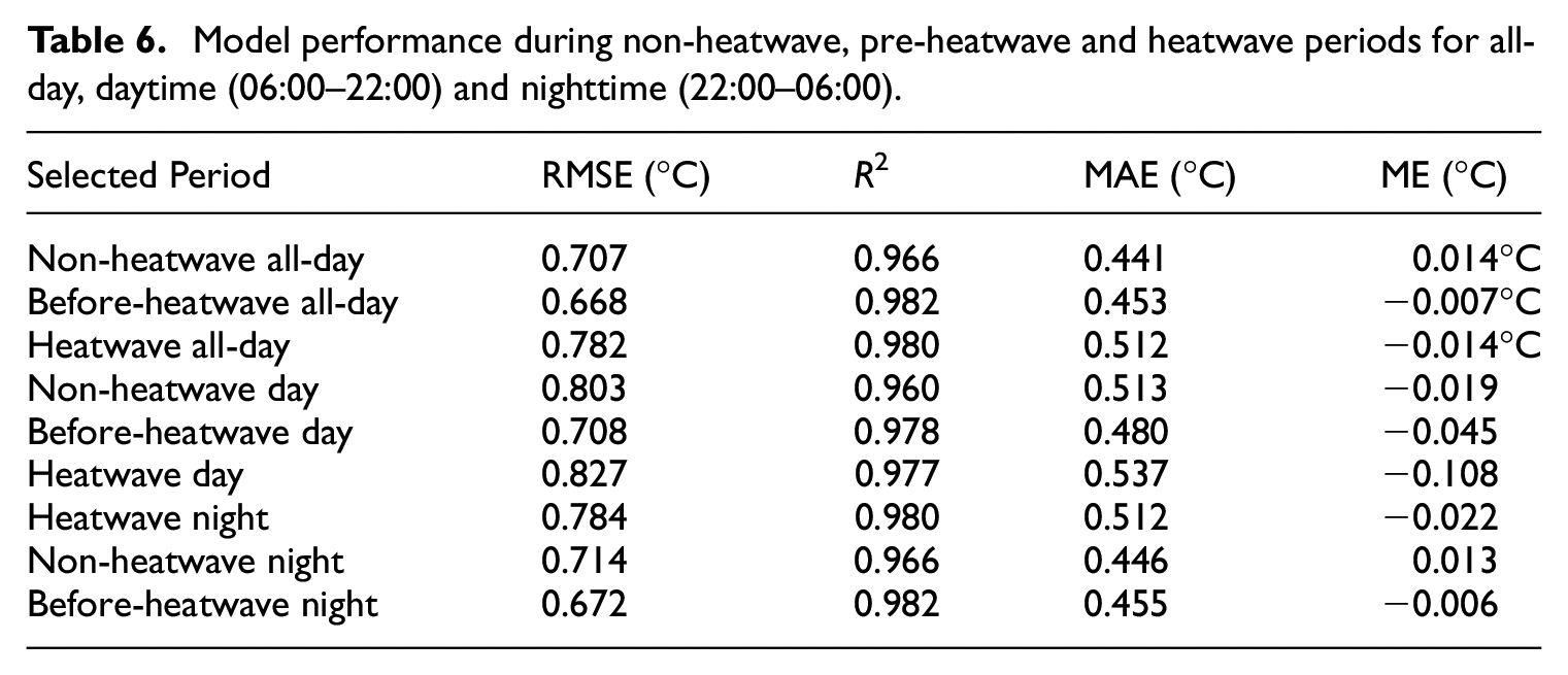
One of the possible reasons for the worse performance during the heatwave than the other periods might be the type of sensors used for ground truth data. These are passively ventilated measurement devices. Although the white color of the case reduces the impact of radiation, a tendency toward overprediction of the air temperature is highly probable due to limited ventilation.

Figure 7 aggregates the difference between the measurements and the WRF-only and WRF + ML approaches into hourly box plots over the whole simulation period. The WRF-only approach underpredicts the temperature in the mornings but overpredicts the evening temperature. By applying our machine learning model, we can eliminate this bias completely, leading to lower RMSE values and a significant increase of the prediction accuracy.

Figure 7.

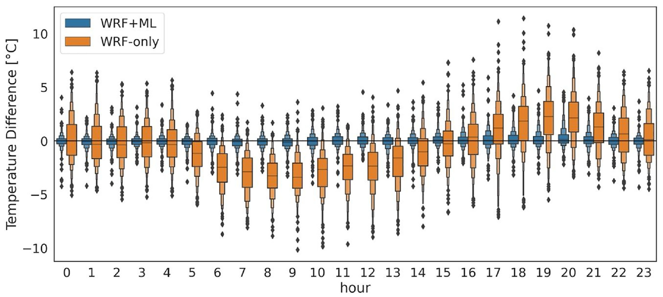
Letter value plot of hourly differences between measurements, WRF-only and WRF + ML for the simulations in Zurich.

We conclude that using available measured data in the city can significantly improve the accuracy of the numerical predictions. This approach of improving WRF with NOAH LSM using ML and measured data shows to be very promising and computationally much less expensive than the use of parametrized urban canopy models, like COSMO-DCEP. The ML approach also does not need static input data as they are already included in the WRF model. A possible future application would be to use also crowdsourcing public measurement networks like Netatmo as input dataset for ML (Coney et al., 2022).

Urban heat island and intra-urban climate analysis

In this chapter, we show the potential of more detailed and accurate mesoscale simulations. We chose two different approaches. The first approach is identifying hot spots by using the heat exposure index. The second approach is an intraurban spatial analysis, considering typical locations with different urban properties.

Urban heat island characterization using heat exposure index

Figure 8(a) shows a map of heat exposure index calculated by WRF data with a threshold temperature of 26°C for the summer period of 2019 for the Zurich agglomeration. The highest heat exposure values are observed for the city center, for the agglomerations along the lake of Zurich and the extensions of the city along the valleys surrounding the city of Zurich. Figure 8(b) shows a map of soil sealing by asphalt or concrete pavements based on (CORINE, n.d.), represented as area ratio of impervious surfaces in percentage and Figure 8(d) shows the average vegetation height (Ginzler, 2021). We observe a positive correlation between soil sealing and heat exposure, and a negative correlation between vegetation height and heat exposure, which indicates that dense urban areas with less greenery show higher air temperatures and heat exposure. Overall, we note that the heat exposure attains values of 4000 dh in the center of Zurich compared to values lying between 2000 and 3000 dh for the suburban areas and of less than 2000 dh in rural areas. Figure 8(c) shows the relative increase of the heat exposure for the urban environment compared to the rural area. The urban and rural areas are defined based on land-use categories as used in WRF. We exclude all urban areas and water bodies for the calculation of a rural average. We then calculate the relative difference in heat exposure between the rural average and the local heat exposure values. We observe that parts of the city of Zurich and its surrounding agglomeration show 150% higher values, meaning that heat exposure is twice the heat exposure of the surrounding rural area.

Figure 8.

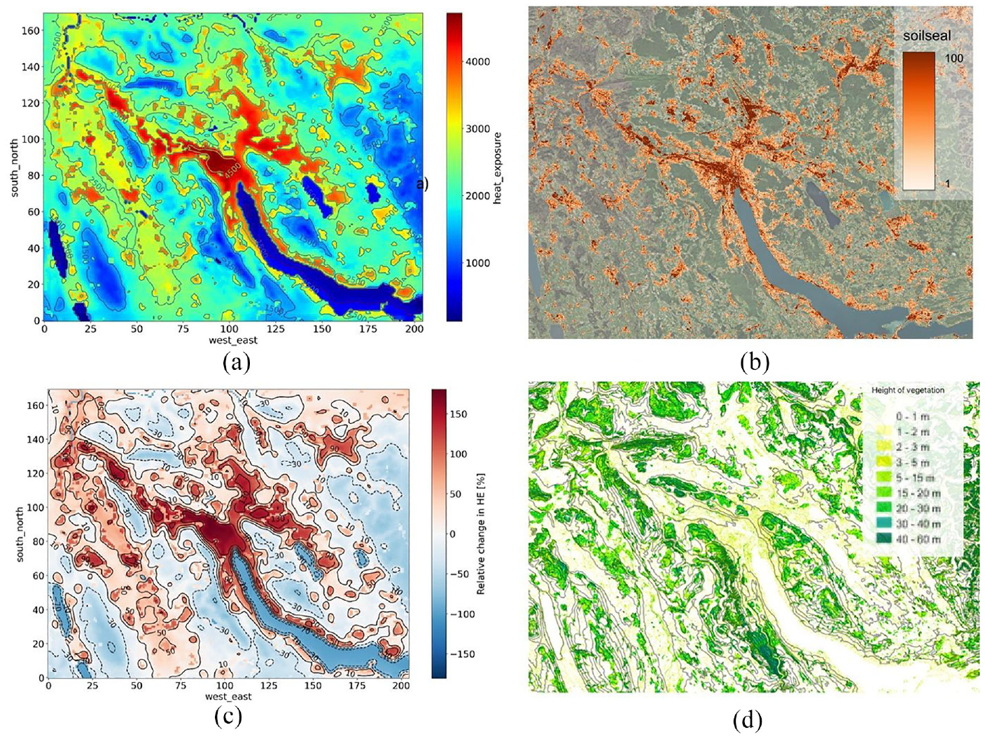
(a) Heat exposure map for Zurich with a threshold temperature of 26°C from June 1st until July 31st, 2019, (b) soil sealing in % based on CORINE (n.d.), (c) relative change of heat exposure between local heat exposure and average rural environment in %, and (d) vegetation height from Swiss National Forest Inventory (Ginzler, 2021) overlaid with altitude contour lines (interval 50 m).

Heat exposure maps with a threshold temperature 23°C are showed in Appendix A5 (Figures A3 and A4). The patterns are similar, and the difference between rural and urban areas is even larger.

Urban heat island and intra-urban climate analysis

The heat exposure maps show quite some intra-urban differences. Therefore, we analyze the spatial distribution of the air temperature averaged over the pre-heatwave (build-up phase), heatwave, and post-heatwave periods as marked in Figure 6 for the period from July 14th until August 1st, 2019. In addition, we divide the different periods into day- and nighttime phases, lasting from 06:00 until 21:00 and from 21:00 until 06:00, respectively. Maps of the average air temperature for these six periods are shown in Figure 9.

Figure 9.

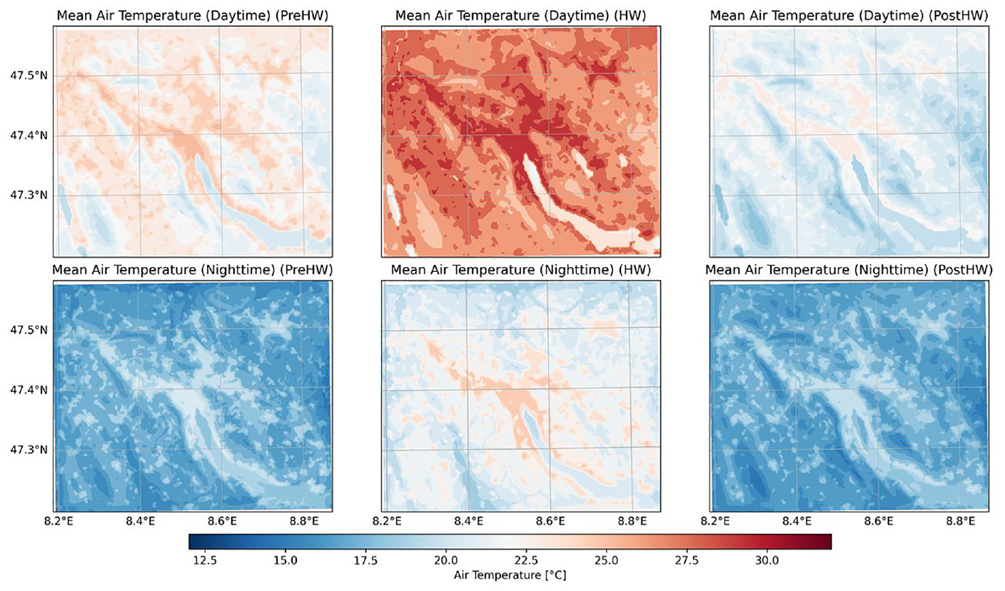
Average daytime and nighttime air temperature during pre-heatwave, heatwave, and post-heatwave periods.

In all maps, a distinct urban heat island effect is clearly visible. The strongest UHI effect is experienced during nighttime under heatwave and pre heatwave conditions where the urban area is on average 1.96°C and 1.97°C hotter than the rural surrounding. One can note the high air temperature in the city during the night of around 25°C. This is significantly above the threshold of a so-called tropical night in Switzerland which is 20°C. Tropical nights affect the well-being of the population considerably and limit the potential of passive nighttime cooling (Rippstein et al., 2023). A strong UHI effect is measured during a heatwave on daytime of about 1.8°C. A strong UHI effect is also experienced during the nights in post-heatwave conditions when we see an UHI effects of about 1.78°C on average. At daytime, in pre- and post-heatwave, the UHII amounts to about 1.5°C albeit with a significantly colder background temperature than during a heatwave. Especially air temperatures and but also UHII are clearly higher during the heatwave period, both during day and night. In combination these two parameters describe the heat stress but also the cooling potential with respect to the rural environment. These are spatial and temporal averages, local maxima can be significantly higher.

In a second intra-urban climate analysis, we compare time series of air temperature from July 14th until August 1st, 2019, for four different urban locations in the city and a rural reference station in the north of the city outside the Zurich highway ring. A map with the different locations is given in Figure 10. The different urban locations are:

Railway Tracks: An urban location in the center of Zurich with low albedo and high thermal capacity. This is the main section of the east-west railway line in Switzerland.

Lake: An urban location at the shore of the lake of Zurich.

Cemetery: A location in the main cemetery of Zurich, which is one of the biggest green areas in the city.

Oerlikon: A sub-urban location in the northern part of Zurich. This location is about 40 m higher than the city center.

Figure 10.

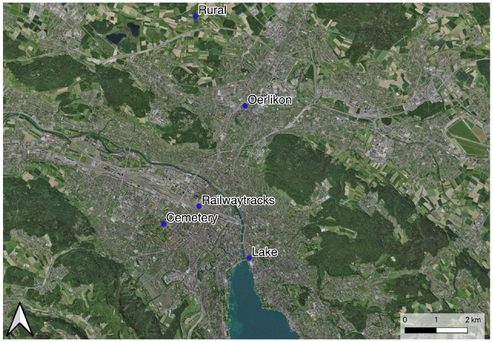
Map of the different locations for the intra-urban analysis in space and time.

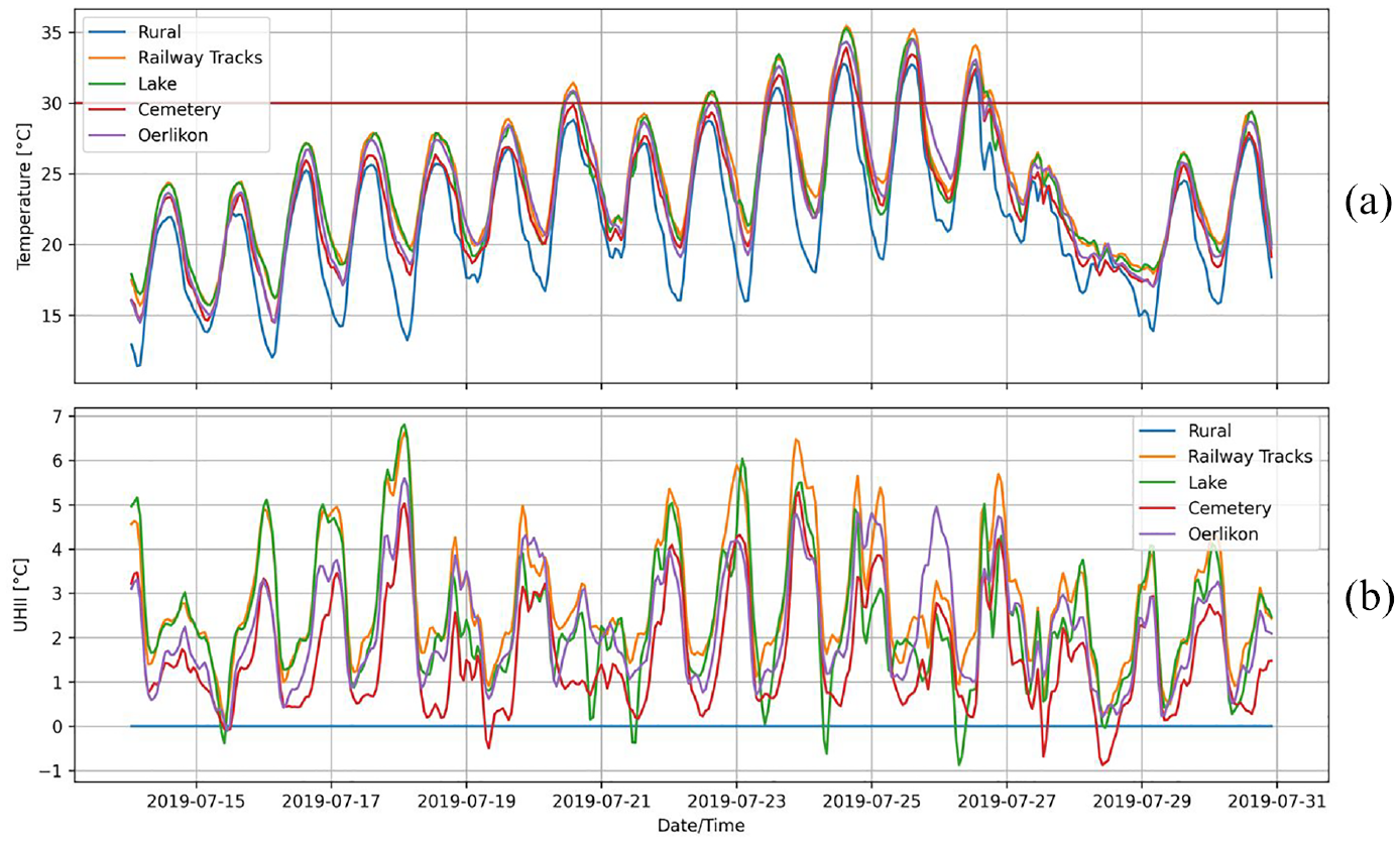
Figure 11 shows the air temperature for all sites during the selected period and the difference in air temperature between the respective urban and rural stations to represent the urban heat island effect. Both subplots are smoothed with a Gaussian filter with $σ = 0.7$ (air temperature) and $σ = 1$ (UHII) for better readability and clarity.

Figure 11.

(a) Air temperature at 2 m height at all selected locations and (b) the UHII at the urban sites against the rural location.

In general, we see that the air temperatures are ramping up over several days before the heatwave, display a certain plateau between July 22nd and July 26th, and decrease rapidly after the heatwave. A similar ramping up of temperature toward a heatwave has also been observed in Mussetti (2020a) and Kong et al. (2023) and was attributed to the fact that, during this pre-heatwave period, more heat is stored than released by materials, leading to an increase in sensible heat transport from hot urban surfaces to the air causing high air temperatures. The UHII also shows higher values during the heatwave days compared to non-heatwave days, showing the synergetic effect between heatwave and UHI (an amplification greater than the sum of the single elements), as reported by Kong et al. (2021). However, high UHII values can also be observed during the pre-heatwave period, with lower values during the post-heatwave period.

Comparing all sites, the rural station outside the city shows almost always the lowest temperatures. During the heatwave, the highest temperatures during daytime are observed for the sites Railway Tracks and Lake. The higher temperature for the Railway Tracks site can be attributed to the use of heavy materials for the tracks and the necessary lack of vegetation. The Lake site shows quite a high built area ratio and low permeable surface ratio. However, during the mornings in the heatwave period the Lake site is significantly colder than railway tracks, leading even to a negative UHII during the 24th of July, meaning it is even cooler than the rural site. This can be explained by the fact that this site experiences cooling from the lake caused by the thermal buffer effect of the water of the lake. The Cemetery site with a lot of greening presents the lowest diurnal amplitude in air temperature, albeit on a higher level than the rural site. This site represents the best thermal comfort of the five urban locations considered here. This site also shows negative UHII values for some instances which means that this location is cooler than the rural site, possibly due to additional cooling by shading and unsealed surfaces. The air temperature in the Oerlikon site is before and after the heatwave closely aligned with the temperature at the Railway Tracks and Lake site. However, through the heatwave, the Oerlikon site is 1°C cooler than those other sites.

In general, we see intra-urban differences of up to 4°C during early morning in heatwave conditions. On average over the whole period, the biggest average intra-urban difference is 1.25°C between the Railway Tracks and the Cemetery site.

Conclusions

Understanding the urban climate, the urban heat island effect and its impacts are key elements for guaranteeing a sustainable and comfortable living in cities around the globe. Moreover, due to climate change, this topic is attracting nowadays much more attention. Since urban climate simulations by MMM with urban parametrizations can become computationally expensive and spatial climate measurement data is scarce, it becomes difficult to identify local hotspots in cities, to understand their origin and to develop adequate mitigation measures.

In this paper, we introduce a new hybrid method to improve mesoscale meteorological simulations of the urban environment. This approach is based on common WRF simulations with an added machine learning algorithm trained by measured urban climate data from a sensor grid in the domain of interest. It is shown that the accuracy of the results can improve significantly. It is also shown how these improved simulations can be used to determine the heat exposure, an insightful time-based index for evaluating hot spots in the urban environment. These improvements reduce the simulation complexity and can help researchers and governmental agencies to assess hot spots more quickly and with higher spatial and temporal accuracy in a city. With a broader deployment of sensor networks in cities it will be possible to use this hybrid method in more cities. It is also possible to harvest citizen science networks like Netatmo Weathermap (an open sharing and publishing platform for weather data) and use the data for training and validation of the model.

We also introduce heat exposure as a new metric to assess local hotspots at mesoscale in cities, and which is similar to indices such as cooling degree days or hours used in building physics. With this heat exposure index, it is possible to detect spatial variability of the urban heat island effect and evaluate different parts of cities for future spatial planning and densification. We show a clear spatial correlation between sealed areas and heat exposure index. Comparing the rural average heat exposure, one can assess the relative increase in heat exposure between city and its environment. Furthermore, we show the intra-urban microclimatic differences of a typical mid-latitude city, indicating the importance of the availability of detailed microclimate simulations in building physics to determine building cooling energy demand accurately. The observed intra-urban magnitudes highlight the need for urban climate data with high accuracy and supports the use of machine learning postprocessing of MMM results.

A possible next research step is to transfer the hybrid model from one city to another and investigate the performance in a completely new setting. Furthermore, one could optimize the design of sensors networks for broad application in cities. Finally, these improved results of the local climate can be used for further building physics analyses, such as the study of impact of energy efficiency measures, durability of building envelopes, indoor thermal comfort, ventilation of buildings, heating and cooling energy demand, and public health studies.

Footnotes

Appendices

Appendix A2. MODIS land use categories for Zurichin domain D03

Table A1.

Description of MODIS land use categories.

Land use category	Description
1	Evergreen Needleleaf Forest
2	Evergreen Broadleaf Forest
3	Deciduous Needleleaf Forest
4	Deciduous Broadleaf Forest
5	Mixed Forests
6	Closed Shrublands
7	Open Shrublands
8	Woody Savannas
9	Savannas
10	Grasslands
11	Permanent Wetlands
12	Croplands
13	Urban and Built-Up
14	Cropland/Natural Vegetation Mosaic
15	Snow and Ice
16	Barren or Sparsely Vegetated
17	Water

Appendix A3. Feature importance for variables

This plot shows the mean decrease in impurity (MIDI), or Gini feature importance, of the 10 most important WRF variables in the ML model. The Gini importance describes how much the model performance would decrease if we would choose a variable randomly.

Appendix A4. Model performance indices

The root mean squared error (RMSE) is defined as:

R M S E = \sqrt{\frac{1}{n} \sum_{i = 1}^{n} {({\hat{y}}_{i} - y_{i})}^{2}}

where ${\hat{y}}_{i}$ is the predicted i-th value and $y_{i}$ i-th ground truth value and n the total number of samples.

R² or coefficient of determination is defined as:

R^{2} = \frac{\sum_{i}^{n} {({\hat{y}}_{i} - \bar{y})}^{2}}{\sum_{i}^{n} {(y_{i} - \bar{y})}^{2}}

where ${\hat{y}}_{i}$ is the predicted i-th value, $y_{i}$ the i-th predicted value, $\bar{y}$ the mean ground truth value, and n the total number of samples.

The mean absolute error (MAE) is defined as:

M A E = \frac{1}{n} \sum_{i = 1}^{n} | {\hat{y}}_{i} - y_{i} |

where ${\hat{y}}_{i}$ is the predicted i-th value, $y_{i}$ the i-th predicted value, and n the total number of samples.

The mean error or model bias is defined as:

M E = \frac{1}{n} \sum_{i = 1}^{n} {\hat{y}}_{i} - y_{i}

where ${\hat{y}}_{i}$ is the predicted i-th value, $y_{i}$ the i-th predicted value, and n the total number of samples.

Appendix A5. Heat exposure maps for a threshold temperature of 23°C

Declaration of conflicting interests

The author(s) declared no potential conflicts of interest with respect to the research, authorship, and/or publication of this article.

Funding

The author(s) received no financial support for the research, authorship, and/or publication of this article.

ORCID iDs

Dominik Strebel

Aytaç Kubilay

References

Baum

Sintermann

(2021) Stadtklimamessungen: Ausgewählte Resultate Sommer 2020. Kanton Zurich, Zurich: AWEL. Available at: https://www.zh.ch/content/dam/zhweb/bilder-dokumente/themen/umwelt-tiere/klima/stadtklima/stadtklima_messnetz_messbericht_2020.pdf

Beck

Zimmermann

McVicar

, et al. (2018) Present and future Köppen-Geiger climate classification maps at 1-km resolution. Scientific Data 5: 180214.

Boudali Errebai

Strebel

Carmeliet

, et al. (2022) Impact of urban heat island on cooling energy demand for residential building in Montreal using meteorological simulations and weather station observations. Energy and Buildings 273: 112410.

Bröde

Fiala

Błażejczyk

, et al. (2012) Deriving the operational procedure for the Universal Thermal Climate Index (UTCI). International Journal of Biometeorology 56(3): 481–494.

Carmeliet

Derome

(2024) How to beat the heat in cities through urban climate modelling. Nature Reviews Physics 6(1): 2–3.

Coney

Pickering

Dufton

, et al. (2022) How useful are crowdsourced air temperature observations? An assessment of Netatmo stations and quality control schemes over the United Kingdom. Meteorological Applications 29(3): e2075.

Copernicus Land Monitoring Service (2009) Imperviousness density 2009 (raster 20 m), Europe, 3-yearly, April 2018. Available at: https://sdi.eea.europa.eu/catalogue/copernicus/api/records/61a2a6c8-9f9a-407d-a01d-d2101e9dcd65 (accessed 5 December 2023).

Copernicus Land Monitoring Service (2020) CORINE Land cover 2012 (raster 100 m), Europe, 6-yearly – version 2020_20u1, May 2020. Available at: https://sdi.eea.europa.eu/catalogue/copernicus/api/records/a84ae124-c5c5-4577-8e10-511bfe55cc0d (accessed 5 December 2023).

CORINE (n.d.) Imperviousness—Copernicus Land Monitoring Service. Available at: https://land.copernicus.eu/pan-european/high-resolution-layers/imperviousness (accessed 23 June 2021).

10.

Davies

(1976) A lateral boundary formulation for multi-level prediction models. Quarterly Journal of the Royal Meteorological Society 102(432): 405–418.

11.

Doms

Baldauf

(2011) A description of the nonhydrostatic regional COSMO model. Part I: Dynamics and numerics. Deutscher Wetterdienst, Offenbach. Epub ahead of print September 2011.

12.

Easterling

Evans

Groisman

, et al. (2000) Observed variability and trends in extreme climate events: A brief review. Bulletin of the American Meteorological Society 81(3): 417–426.

13.

Federal Office of Statistics (2022) City statistics porträts 2022: Agglomerationen. Swiss Federal Office of Statistics. Available at: https://www.bfs.admin.ch/bfs/en/home/statistics/cross-sectional-topics/city-statistics/city-portraits/zurich.html (accessed 4 December 2023).

14.

Fischer

(2023) Technischer Bericht zum Nationalen Beobachtungsnetz für Luftfremdstoffe (NABEL) 2023. Bern: Swiss Federal Office of the Environment.

15.

Ginzler

(2021) Vegetation height model NFI. National Forest Inventory (NFI). Available at: https://envidat.ch/#/metadata/vegetation-height-model-nfi (accessed 8 December 2023).

16.

Heaviside

Macintyre

Vardoulakis

(2017) The urban heat Island: Implications for health in a changing environment. Current Environmental Health Reports 4(3): 296–305.

17.

Hersbach

Bell

Berrisford

, et al. (2020) The ERA5 global reanalysis. Quarterly Journal of the Royal Meteorological Society 146(730): 1999–2049.

18.

Hintz

Luederitz

Lang

, et al. (2018) Facing the heat: A systematic literature review exploring the transferability of solutions to cope with urban heat waves. Urban Climate 24: 714–727.

19.

Hondula

Kuras

Betzel

, et al. (2021) Novel metrics for relating personal heat exposure to social risk factors and outdoor ambient temperature. Environment International 146: 106271.

20.

Kong

Zhao

Carmeliet

, et al. (2021) Urban heat island and its interaction with heatwaves: A review of studies on mesoscale. Sustainability 13(19): 10923.

21.

Kong

Zhao

Strebel

, et al. (2023) Understanding the impact of heatwave on urban heat in greater Sydney: Temporal surface energy budget change with land types. Science of the Total Environment 903: 166374.

22.

Kubilay

Allegrini

Strebel

, et al. (2020) Advancement in urban climate modelling at local scale: Urban heat Island mitigation and building cooling demand. Atmosphere 11(12): 1313.

23.

Kubilay A and OpenFOAM Community (2024) UrbanMicroclimateFoam—an open-source solver for coupled physical processes modeling urban microclimate based on OpenFOAM. Available at: https://gitlab.ethz.ch/openfoam-cbp (accessed 5 December 2023).

24.

Kusaka

Kondo

Kikegawa

, et al. (2001) A simple single-layer urban canopy model for atmospheric models: Comparison with multi-layer and slab models. Boundary-Layer Meteorology 101(3): 329–358.

25.

Lass

Haas

Hinkel

, et al. (2011) Avoiding the avoidable: Towards a European heat waves risk governance. International Journal of Disaster Risk Science 2(1): 1–14.

26.

Zhao

Bardhan

, et al. (2023) Relating three-decade surge in space cooling demand to urban warming. Environmental Research Letters 18(12): 124033.

27.

Manickathan

Defraeye

Allegrini

, et al. (2018) Parametric study of the influence of environmental factors and tree properties on the transpirative cooling effect of trees. Agricultural and Forest Meteorology 248: 259–274.

28.

Martilli

Clappier

Rotach

(2002) An urban surface exchange parameterisation for mesoscale models. Boundary-Layer Meteorology 104(2): 261–304.

29.

Masson

(2000) A physically-based scheme for the urban energy budget in atmospheric models. Boundary-Layer Meteorology 94(3): 357–397.

30.

McCarthy

and Intergovernmental Panel on Climate Change (eds) (2001) Climate Change 2001: Impacts, Adaptation, and Vulnerability: Contribution of Working Group II to the Third Assessment Report of the Intergovernmental Panel on Climate Change. Cambridge; New York, NY: Cambridge University Press.

31.

Mirzaei

(2021) CFD modeling of micro and urban climates: Problems to be solved in the new decade. Sustainable Cities and Society 69: 102839.

32.

Moonen

Defraeye

Dorer

, et al. (2012) Urban physics: Effect of the micro-climate on comfort, health and energy demand. Frontiers of Architectural Research 1(3): 197–228.

33.

Mussetti

Brunner

Allegrini

, et al. (2020a) Simulating urban climate at sub-kilometre scale for representing the intra-urban variability of Zurich, Switzerland. International Journal of Climatology 40(1): 458–476.

34.

Mussetti

Brunner

Henne

, et al. (2020b) COSMO-BEP-Tree v1.0: A coupled urban climate model with explicit representation of street trees. Geoscientific Model Development 13(3): 1685–1710.

35.

NASA (2019a) ASTER global digital elevation model V003. NASA EOSDIS Land Processes Distributed Active Archive Center. Available at: https://lpdaac.usgs.gov/products/astgtmv003/ (accessed 5 December 2023).

36.

NASA (2019b) Urban heat Islands. My NASA data. Available at: https://mynasadata.larc.nasa.gov/basic-page/urban-heat-islands (accessed 21 December 2023).

37.

Oke

(1982) The energetic basis of the urban heat Island. Quarterly Journal of the Royal Meteorological Society 108(455): 1–24.

38.

Orlanski

(1975) A rational subdivision of scales for atmospheric processes. Bulletin of the American Meteorological Society 56(5): 527–530.

39.

Ragettli

Saucy

Flückiger

, et al. (2023) Explorative assessment of the temperature–mortality association to support health-based heat-warning thresholds: A national case-crossover study in Switzerland. International Journal of Environmental Research and Public Health 20(6): 4958.

40.

Rippstein

de Schrijver

Eckert

, et al. (2023) Trends in tropical nights and their effects on mortality in Switzerland across 50 years. PLoS Climate 2(4): e0000162.

41.

Salamanca

Martilli

Tewari

, et al. (2011) A study of the urban boundary layer using different urban parameterizations and high-resolution urban canopy parameters with WRF. Journal of Applied Meteorology and Climatology 50(5): 1107–1128.

42.

Schubert

Grossman-Clarke

Martilli

(2012) A double-canyon radiation scheme for multi-layer urban canopy models. Boundary-Layer Meteorology 145(3): 439–468.

43.

Sensirion (2022) Datasheet SHT3x. Available at: https://sensirion.com/media/documents/213E6A3B/63A5A569/Datasheet_SHT3x_DIS.pdf (accessed 7 December 2023).

44.

Silva

Eggimann

Fierz

, et al. (2022) Opportunities for passive cooling to mitigate the impact of climate change in Switzerland. Building and Environment 208: 108574.

45.

Skamarock

Klemp

Dudhia

, et al. (2019) A Description of the Advanced Research WRF Model Version 4.3. Boulder, Colorado: National Center for Atmospheric Research Technical Notes.

46.

Statistik Zurich (2023) Bevölkerungsbestand und -entwicklung—Stadt Zürich. Available at: https://www.stadt-zuerich.ch/prd/de/index/statistik/themen/bevoelkerung/bevoelkerungsentwicklung/aktueller-bevoelkerungsbestand.html (accessed 4 December 2023).

47.

Swisstopo (2010) SwissBUILDINGS3D 1.0. Available at: https://www.geocat.ch/geonetwork/srv/api/records/4d4544b1-d57b-4ccc-b69d-582198286692 (accessed 5 December 2023).

48.

Swisstopo Landeskarte 1:25000 (2023) Landeskarte 1:25’000—opendata.swiss. Available at: https://opendata.swiss/de/dataset/landeskarte-1-25000 (accessed 30 January 2024).

49.

Toparlar

Blocken

Maiheu

, et al. (2017) A review on the CFD analysis of urban microclimate. Renewable and Sustainable Energy Reviews 80: 1613–1640.

50.

WHO Heatwaves (2004) Heatwaves. Available at: https://www.who.int/health-topics/heatwaves (accessed 17 January 2024).

51.

WRF User’s Guide (2020) WRF (ARW) version 4.0 user’s guide. Available at: https://www2.mmm.ucar.edu/wrf/users/docs/user_guide_v4/v4.2/WRFUsersGuide_v42.pdf (accessed 15 December 2023).

52.

Wang

Liu

, et al. (2020) The record-breaking heat wave of June 2019 in Central Europe. Atmospheric Science Letters 21(4): e964.

53.

Zhao

Sen

Susca

, et al. (2023) Beating urban heat: Multimeasure-centric solution sets and a complementary framework for decision-making. Renewable and Sustainable Energy Reviews 186: 113668.

Improved mesoscopic meteorological modeling of the urban climate for building physics applications

Abstract

Keywords

Introduction

Heatwave analysis over the last 30 years in Zurich

Mesoscale Meteorological Modeling (MMM) of a summer urban climate in Zurich

Description of the Mesoscale Meteorological Models (MMM)

Validation of the COSMO-DCEP and WRF-NOAH MMM models

Improved WRF model using machine learning (ML)

Urban heat island and intra-urban climate analysis

Urban heat island characterization using heat exposure index

Urban heat island and intra-urban climate analysis

Conclusions

Footnotes

Appendices

Appendix A2. MODIS land use categories for Zurichin domain D03

Appendix A3. Feature importance for variables

Appendix A4. Model performance indices

Appendix A5. Heat exposure maps for a threshold temperature of 23°C

Declaration of conflicting interests

Funding

ORCID iDs

References