Sage Journals: Discover world-class research

Abstract

In order to optimize the energy requirements (heating/cooling) of a multi-zone greenhouse, and investigate its heat recovery potential, a mathematical, dynamic energy model, coded in the MATLAB/Simulink platform, is developed. For validation, a case study in cold climate conditions is evaluated. This dynamic model, based on both energy and water vapor mass balances, was able to calculate the year-round monthly energy demand for the case study. The model calculations were compared with actual energy consumption data and were shown to have an accuracy between 6% and 15.5% for different months. The results highlighted the potential of applying a heat recovery strategy, whether with a Phase Change Material (PCM) or a Heat Recovery Ventilator (HRV). It is shown that using a HRV can reduce the energy demand of the greenhouse by 5% for January and 4% for December. Regarding the greenhouse radiation performance, the south roof contributes the most to solar heat gain in winter and summer, while the north wall makes the minimum contribution. Consequently, it is proposed to increase the area of the south roof and insulate the north wall. Thus, an asymmetrical roof configuration can receive 6% more solar radiation. Calculations show that an east-west greenhouse orientation lowers energy demand by 3%.

Keywords

Greenhouse model multi-zone cold climate solar radiation heat recovery

Introduction

Currently, most countries are suffering from a huge shortage in sustainable food and energy resources. This situation is due in part to COVID-19, extreme weather conditions, and the ravages of war. Greenhouses are the most effective solution for the ever-increasing demand for sustainable agriculture (Ahamed et al., 2019). However, greenhouse energy consumption, which can be significantly higher than that of conventional cultivation, can affect the benefits of industrial farming (Barbosa et al., 2015). Beshada et al. (2006) focused on the energy consumption of greenhouses, and confirmed the vast amount of energy that they onsum. Generally, greenhouses are considered as a solar collector system, which means that by optimizing their properties (dimensions, orientation, materials, etc.) a net zero energy greenhouse in achievable (Vadiee and Martin, 2014; van ’t Ooster et al., 2007). The design parameters of a greenhouse are highly dependent on climate conditions. This topic was extensively reviewed by Ghani et al. (2019). Zaragoza et al. (2007) proposed a closed concept solar greenhouse that in addition to reducing energy consumption, has advantages such as lower operating cost, recovery of low-quality water (gray water), and lower air pollution. To have the highest productivity in arid regions such as the Middle East or Southern Europe, where farmers face obstacles such as extreme air temperature, insufficient water supply resources, and poor soil quality, a seawater greenhouse system (Al-Ismaili and Jayasuriya, 2016) has been proposed. Based on a thermal storage concept, the Chinese style greenhouse configuration (Gao et al., 2010; Tong et al., 2013) allows removal or reduction of the external heating utility.

To find potential solutions for reducing the energy consumption of a solar greenhouse in northern regions, developing a mathematical energy model is a key step. However, developing this model could be a very sophisticated task. To calculate the energy demand, the contribution of the most important factors must be taken into the account, including the type of plants (tomato, potato, roses, poinsettia, etc.), soil properties, interior air conditions (temperature set point, relative humidity, etc.), greenhouse structure, outdoor climate (temperature, wind speed, solar radiation, etc.), and greenhouse orientation. In fact, the number of considered factors largely determines to what extent a model is accurate and functional. Such a mathematical model with numerous parameters and their dynamic behavior will undoubtedly be very complex. The principal purpose of this model is to calculate the heat and mass transfer rates within a greenhouse. Having an accurate energy model enables energy analysts and researchers to propose appropriate strategies to target the minimum energy consumption and operating cost.

Early studies regarding the development of energy models for greenhouses date back to the 1980s when, to calculate the energy demand of a greenhouse, Bot (1988) utilized an energy model that considered the greenhouse cover, air, crop canopy, and four layers of soil. Later, this study was improved by Takakura (1993). In another study, with the objective of optimizing the net profit of a tomato greenhouse, Trigui et al. (2001) utilized a dynamic energy model to compute the heating/cooling load of a greenhouse. They proposed a multi-step approach, in which the first step was defining the profit. They defined the profit as the crop yield value less the energy costs, for heating and dehumidification, and the CO2 injection cost. Then, in the second step, they proposed an algorithm with a Hamiltonian function to solve the objective function J, which maximizes the net profit during harvest time.

De Zwart (1996) and later Luo et al. (2005) proposed a mathematical model based on an energy and mass balance which was capable of predicting the energy demand, humidity, temperature, and CO2 concentration within a greenhouse. Also, Golzar et al. (2018) proposed an integrated mathematical model that calculates both the energy demand of a greenhouse as well as the crop growth, including models for both. They studied and accounted for the interaction between energy consumption and crop yield. Also, they reviewed 30 different energy models for greenhouses. Esmaeli and Roshandel (2020) proposed a new energy model, based on climate conditions of Iran, and optimized a greenhouse where cucumbers, melons, and watermelons are cultivated. However, they did not consider the effect of the type of product on energy demand. Chen et al. (2015) used hybrid particle swarm optimization and a genetic algorithm (HPSO-GA) technique to optimize the energy demand of a greenhouse. They concluded that PSO would bring more accurate and reliable results for dynamic parameters. The dynamic model developed by Mohammadi et al. (2018) was capable of predicting the inside air and soil temperature.

There are two other computer-based simulation approaches that have been applied by researchers in their efforts to predict the thermal load of greenhouses. The first one is Building Energy Modeling (BEM) commercial software like EnergyPlus and more importantly TRNSYS. However, their ability to predict the greenhouse’s parameters is questionable. Commercial software mostly suffers from its inability to consider specific greenhouse phenomena such as evaporation and plant transpiration (evapotranspiration), which barely occur in residential or commercial buildings. For example, water moisture production in a greenhouse is a function of solar radiation, plant type, total plant floor coverage, plant growth, watering schedule, etc. Also, most practical greenhouses are equipped with thermal and blackout screens. Building software packages are unable to accurately simulate these features or account for several of the named greenhouse parameters. Another issue with commercial software is that the user is very limited in the ability to manipulate the software’s mathematical formulas. Having said that, while commercial software products can consider multi-zone features, the mentioned limitations make them an unreliable tool for greenhouse modeling and design. Ahamed et al. (2020) used TRNSYS software to obtain the energy demand of a greenhouse. However, his study revealed that this software is completely unable to produce accurate data. As another example, Chen et al. (2018) used EnergyPlus software to optimize a Chinese style greenhouse’s north wall to have maximum solar radiation in order to target minimum energy demand. The second simulation approach, which has significant capability but is very case dependent, is computational fluid dynamics (CFD). Using CFD, Zhang et al. (2016) obtained the temperature and moisture distribution within a Chinese style greenhouse. They used an ANSYS package to solve the 2-D Navier-Stokes equations with dynamic boundary conditions to obtain operational data within a greenhouse.

Previous studies considered the greenhouse as a single micro-climate, whereas in practice greenhouses are typically subdivided into several zones, each with their own temperature and humidity setpoints. Hereafter, this kind of greenhouse will be referred to as “multi-zone.” Multi-zone greenhouses can potentially provide an important opportunity for energy saving and heat recovery. In this study, an in-house MATLAB-Simulink code, which was previously validated by this research team (Ghaderi et al., 2023), is selected as the starting point. The earlier code was only able to predict the heat load of a single micro-climate zone greenhouse, and did not consider the effect of artificial lighting, thermal screens, and fans. Hence, the current study has two main objectives. The first objective it to develop and present a mathematical energy model for calculating the energy demand (heating/cooling load as well as dehumidification load) of a multi-zone greenhouse in a northern growing region. This model will consider thermal screens, artificial lighting, and equipment loads. To the best knowledge of the authors, no previous studies presented an energy model that calculates the energy demand of a multiple micro-climate greenhouse. By developing this energy model, the opportunities for taking advantage of heat recovery or heat storage in different zones can be investigated. The second objective is to propose the best physical properties of a greenhouse in cold climate agricultural regions, such as Quebec, Canada.

Model development

In the following sections, after introducing the governing equations and the properties of a chosen case study, the model validation results will be presented. Then, in the results and discussion chapter, the heat recovery potential and solar radiation factors will be investigated.

In this section the formulas that cover the energy and mass conservation in a multi-zone greenhouse are presented. A lumped model was found to be sufficiently accurate to capture the transient behavior of a single-zone greenhouse micro-climate (Van Beveren et al., 2015). A lumped energy model is a simplified representation of a complex physical system, where the system’s behavior is approximated using discrete components characterized by parameters such as mass, capacitance, and resistance. In this model, the system is divided into distinct elements, and interactions between them are defined by simple mathematical equations. The lumped energy model is particularly valuable in engineering and physics for analyzing and predicting the behavior of systems, such as electrical circuits or thermal systems, by focusing on energy storage and dissipation while disregarding spatial variations. Though it offers a streamlined approach to system analysis, it may not account for all real-world complexities in highly distributed or intricately interacting systems.

Energy balance

The overall greenhouse heat balance equation is presented in equation (1). Figure 1 schematically illustrates the different mechanisms that can affect the greenhouse energy consumption. The formulation of each mechanism is described in section 2.1 and 2.2.

ρ_{a} V_{g} C_{a} \frac{d T_{i n} (t)}{d t} = q_{s o l a r} (t) + q_{l i g h t i n g} (t) + q_{f a n} (t) + q_{c o n} (t) + q_{t r a n s} (t) + q_{s o i l} (t) + q_{l} (t) + q_{P} + q_{v e n t} + q_{v e n t M e c h} + q_{D e h}

(1)

Figure 1.

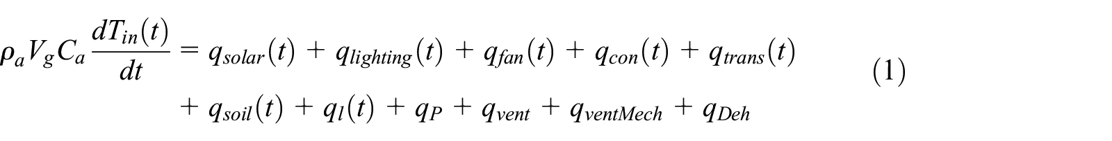
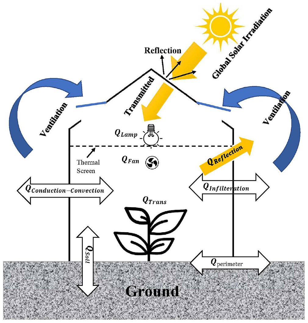
Different heat loss/gain mechanisms in a conventional greenhouse.

In the above equation, T_in(t) is the time dependent temperature of indoor air, C_a is the heat capacity of air, $ρ_{a}$ is the density and q denotes the heat gain and loss mechanisms, which are described in the following section.

In a greenhouse, the main source of heat gain comes from solar radiation. In other word, the greenhouse can be considered as solar collector. The solar radiation $q_{solar} (t)$ passing through the greenhouse cover material is calculated by equation (2) (Duffie and Beckman, 2013).

q_{solar} (t) = [A_{i} I_{i} (t)] τ_{i}

(2)

A _i is the total surface area of the greenhouse cover (m²), I_i (t) is total solar irradiance $(W m^{- 2})$ and τ_i is the transmission coefficient of the greenhouse cover. To calculate the total solar irradiance I_i(t) on a sloped surface, various models have been proposed Ahamed et al. (2018), of which the isotropic sky model is the most recommended. Based on this model, if the sum of diffuse and of reflected radiation from the ground is considered isotropic, the sum of diffuse radiation from the sky and ground reflected radiation on a sloped surface is the same, regardless of their orientation (Duffie and Beckman, 2013). So, the total radiation $I_{i}$ on a sloped surface is equal to the summation of the beam contribution $I_{b}$ and the diffuse radiation on a horizontal surface $I_{d}$ .

After some simplifications, the total amount of solar radiation on a sloped surface $I_{i}$ can be obtained by equation (3) (Liu and Jordan, 1963).

I_{i} = I_{b} \frac{\cos θ_{i}}{\cos θ_{z}} + I_{d} (\frac{1 + \cos β}{2}) + (I_{b} + I_{d}) (\frac{1 - \cos β}{2})

(3)

In equation (3), $β$ , $θ_{i}$ , and $θ_{z}$ are the surface slope angle, the angle of incidence of beam radiation on a surface and the zenith angle of the sun, respectively.

\cos θ_{i} = \cos β \sin δ \sin φ - \cos φ \cos ϒ \sin δ \sin β + \cos φ \cos δ \cos β \cos ω + \cos δ \sin φ \sin β \cos ω \cos ϒ + \cos δ \sin β \sin ω \sin ϒ

(4)

\cos θ_{z} = \cos φ \cos δ \cos ω + \sin δ \sin φ

(5)

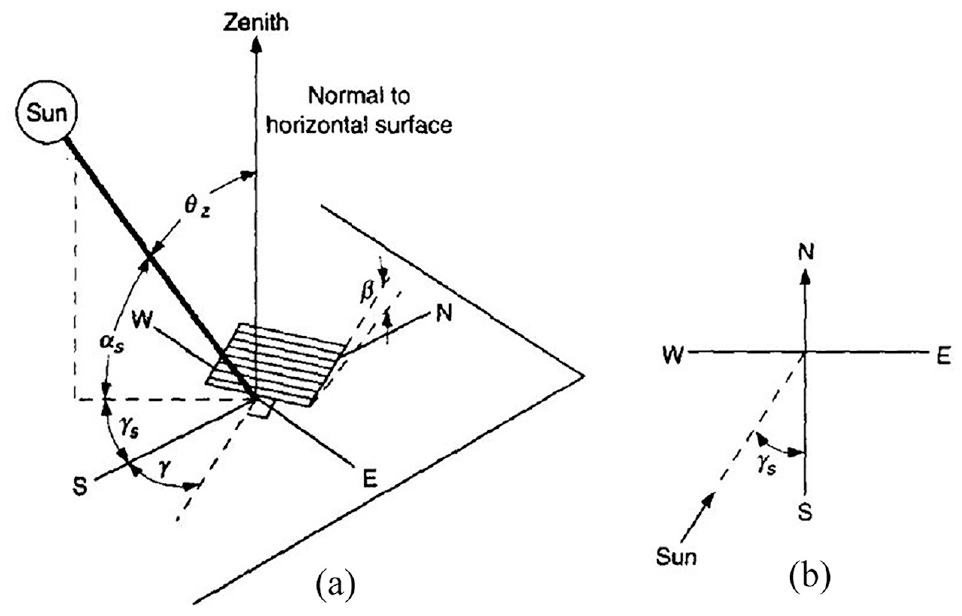
In equations (4) and (5), ω, δ, ϒ, and $φ$ are hour angle, declination angle of sun, surface azimuth angle, and local latitude angle, respectively. Figure 2 illustrates the mentioned angles, schematically.

Figure 2.

(a) Schematic diagram of different angles that affect solar radiation and (b) solar azimuth angle.

Heat transfer rates $q_{lighting}$ (t) and $q_{fan}$ (t) are the contribution of electrical energy transformed into heat by supplementary lamps and fans, which are calculated as:

q_{lighting} (t) = η_{th} P_{E} \frac{f_{on}}{100}

(6-1)

q_{fan} (t) = N_{f} \frac{P_{m}}{E_{m}} F_{um} F_{ul}

(6-2)

where η_th is the thermal ratio of lamps, $P_{E}$ is electric power of artificial lighting ( $W m^{- 2}$ ) and f_on is the fraction of lamps that are on at a given moment. Also, $N_{f}$ , $P_{m}$ , $E_{m}$ , $F_{um}$ , and $F_{ul}$ are number of fans, motor power, motor efficiency, motor load factor, and motor use factor, respectively.

Heat loss due to convection and conduction $q_{con} (t)$ is a function of inside and outside temperature difference and is calculated by equation (7). Note that the heat conduction through soil will be calculated separately. In equation (7), $U_{t}$ and $U_{NT}$ are the heat transfer coefficients of the transparent and non-transparent parts of the greenhouse cover.

q_{con} (t) = (U_{t} A_{t} + U_{NT} A_{NT}) (T_{i} (t) - T_{o} (t))

(7)

U_{t} = {(\frac{1}{h_{i}} + N_{c} \frac{L_{c}}{K_{c}} (N_{c} - 1) \frac{1}{h_{a}} + \frac{1}{h_{0}})}^{- 1}

(8)

U_{NT} = {(\frac{1}{h_{i}} + \sum^{\frac{K_{n}}{Δ x}} + \frac{1}{h_{0}})}^{- 1}

(9)

In equations (8) and (9), $h_{0}$ , $h_{i}$ , $K_{c}$ , $h_{a}$ , and $N_{c}$ represent the convection coefficient for outdoor and indoor surfaces, thermal conductivity of the cover, convection coefficient for air, and number of layers in the covering, respectively. To calculate the value of the mentioned parameters, reference (Clark and Allen, 1978) is utilized. Calculating the value of $h_{a}$ (thermal conductance of the air spaces for a double-layer greenhouse cover) is the first step. Based on a literature review, selecting the value of 3.85 $W m^{- 2} k^{- 1}$ has the highest compliance with experiential results. The next step is selecting a method to calculate the convection coefficient for greenhouse covering surfaces, whether outside or inside.

h = Nu \frac{K_{a}}{L_{c}}

(10)

Since the air velocity inside greenhouses is negligible (less than 0.2 $m s^{- 1}$ ), the convective heat transfer coefficient at the transparent cover inside surface is considered to be free convection. By this assumption, we rewrite equation 10 as follows, in equation 11:

h_{i} = (\frac{K_{a}}{L_{c}}) 0.1 {(G_{r} P_{r})}^{0.33} 10^{9} < G_{r} P_{r} < 10^{13}

(11)

G_{r} = \frac{g \partial {L_{c}}^{3} Δ T}{μ^{2}}

(12)

P_{r} = \frac{μ C_{pa}}{K_{a}}

(13)

In equations (11)–(13), $K_{a}$ , $L_{c}, \partial$ , $g$ , $μ$ , and $C_{pa}$ are the thermal conductivity of air, characteristic length of convective surfaces, volumetric thermal expansion coefficient ( $K^{- 1}$ ), acceleration due to gravity, air viscosity, and specific heat of air ( $Jk g^{- 1} K^{- 1})$ , respectively. Also, $G_{r}$ and $P_{r}$ stand for Grashof number and Prandtl number.

Usually, greenhouses have a non-transparent wall portion on the east, south and west sides, extending upwards from ground level for 60 cm. To calculate the non-transparent vertical surfaces, the indoor convection coefficient can be obtained by equation 14.

h_{i} = 0.1 \frac{K_{a}}{L_{c}} {(10^{11})}^{0.33}

(14)

Since the main heat transfer mechanism on the outside walls is forced convection, the convective heat transfer coefficient can be calculated by equation 15, noting that it mainly depends on the Reynolds and Prandtl numbers.

h_{o} = (\frac{K_{a}}{L_{c}}) 0.037 (R e^{. 8} {P_{r}}^{0.33}) Re > 5 * 10^{5}

(15)

It should be noted that to obtain the Re value, a length-based formulation must be considered (equation 16).

Re = \frac{ρ V_{0} L_{c}}{μ}

(16)

In equation 16, ρ is air density, $V_{0}$ is air velocity, and $L_{c}$ is the surface length. To prepare equation 7 for a multi-zone greenhouse, some adjustments are necessary. Like commercial software, for walls shared between adjacent zones, the boundary conditions need some modifications. To clarify this concept, consider zone 3, which has one shared wall on the north side with zone 2. The north wall of zone 3 (south wall of zone 2) is not exposed to outside temperature, but instead is exposed to the thermal conditions of the adjacent portion of the greenhouse (zone 2). Hence, to calculate the value for conductive heat transfer on the north wall of zone 3, the air temperature of zone 2 should replace the outside temperature. A similar approach is necessary for solving the mass transfer equations. Although these modifications increase the complexity of code, they help increase the code accuracy. The necessity of this modification is greatest during the winter season when the outdoor temperature is negative.

One of the most challenging tasks in developing a mathematical energy model for a greenhouse is modeling mechanical ventilation in open-concept greenhouses. In this study we only considered the natural ventilation, which is responsible of up to 20% of heat lost in a greenhouse (Ahamed et al., 2018).

q_{\inf} (t) = 0.33 N V_{g} (T_{in} - T_{out})

(17)

In the above equation, $N$ and $V_{g}$ represents the number of air exchanges per hour (here, it is considered 1) and the greenhouse volume, respectively.

Greenhouses have different mechanisms to meet the greenhouse thermal load in the winter season. One of these mechanisms is a floor heating system. The greenhouse floor can lose energy in two ways. First, heat conduction to the ground (equation (18)) and second, perimeter heat loss (equation (19)).

q_{soil} = \frac{K_{s}}{H} A_{f} (T_{i} - T_{s})

(18)

q_{p} = F_{p} P (T_{i} - T_{o})

(19)

Thermal radiation q_l(t) from the inside to the outside of the greenhouse, which is also known as long-wave radiation heat loss, is one of the most important heat losses that affects the greenhouse micro-climate. This term is computed by equation (20):

q_{l} (t) = ε_{c} A_{c} σ F_{c} (T_{i}^{4} + T_{c}^{4}) + ε_{i} τ_{l} A_{f} σ F_{sky} (T_{in}^{4} + T_{sky}^{4})

(20)

Where σ is the Stefan–Boltzmann constant ( $W m^{- 2} C^{- 4}$ ), $ε_{c}$ is the emission coefficient of cover, $ε_{i}$ is the emission coefficient of indoor equipment, $F_{sky}$ is the view factor between the greenhouse (equal to 1 (Vadiee, 2011)), and $τ_{l}$ is the transmissivity of the cover to long-wave radiation. The value of $F_{c}$ (the view factor between the ground and the cover) is calculated by equation (21) (Liu and Jordan, 1961). Also, $T_{c}$ is calculated as a function of outdoor and indoor temperatures as equation (22). To calculate $T_{sky}$ the approach of references (Ahamed et al., 2018; Clark and Allen, 1978) is employed.

F_{c} = \frac{1 + \cos θ}{2}

(21)

T_{c} = \frac{2}{3} T_{out} (t) + \frac{1}{3} T_{i} (t)

(22)

In cold regions, greenhouses are equipped with thermal screens to control the mentioned term $q_{l} (t) .$

Plant transpiration affects both the temperature and water content of the greenhouse indoor air. The model that is used in this work is based on the transpiration model of Van Beveren et al. (2015) and is described in equation (23):

q_{trans} (t) = g_{e} (t) l_{v} A (χ_{crop} (t) - χ (t))

(23)

Where $l_{v}$ is the latent energy or the amount of energy required to evaporate water from a leaf surface ( $J m^{- 1}$ ), A is the greenhouse floor area, χ_crop(t) is the absolute water vapor concentration very close to the canopy surface ( $g m^{- 3}$ ), $χ (t)$ is the absolute water vapor concentration of the indoor air ( $g m^{- 3}$ ) and will be calculated at the assumed relative humidity setpoint. The term g_e(t) is the transpiration conductance, which is expressed as:

g_{e} (t) = \frac{2 LAI}{(1 + ε) r_{b} + r_{s} (t)} (m s^{- 1})

(24)

In equation (24), LAI is the Leaf Area Index (m² leaf divided by m² ground), ε is the ratio of latent to sensible heat content of saturated air, $r_{b}$ is the boundary layer resistance parameter ( $s m^{- 1}$ ) and r_s(t) is the stomatal resistance ( $s m^{- 1}$ ) which is calculated by equation (27). $χ_{crop}$ in equation (23) is calculated as:

χ_{crop} (t) = χ_{air, sat} (t) + ε (t) \frac{r_{b}}{2 LAI (t)} \frac{R_{n} (t)}{L}

(25)

Where χ_air,sat(t) is the indoor saturated vapor concentration ( $g m^{- 3}$ ) and R_n(t) is net radiation at crop level ( $W m^{- 2}$ ). The saturated vapor concentration can be approximated as a function of inside temperature as:

χ_{air, sat} (t) = 5 . 5638_{\exp} (0.0572 T_{in} (t))

(26)

Stomatal resistance rs(t) is an index showing the resistance to transpiration of water vapor through the stomata (leaf pores) on the plant leaves and is written follows by a semi-empirical model:

r_{s} (t) = (82 + 570 \exp (- γ \frac{R_{n} (t)}{LAI})) (1 + 0.023 (T_{air} (t) - 24.5)^{2})

(27)

Where γ is a crop specific parameter (e.g. its value is 0.027 for tomato and 0.008 for rose (Van Beveren et al., 2015)). Also, in equation (28), $P_{E}$ is the rated electric power of artificial lighting installed ( $W m^{- 2}$ ):

R_{n} (t) = 0.86 (1 - \exp (1 - 0.7 LAI)) (q_{solar} (t) + P_{E} \frac{f_{on}}{100})

(28)

$q_{vent}$ and $q_{ventMech}$ in equation (1) denote the heat exchange with the environment caused by natural ventilation and mechanical ventilation while $q_{Deh}$ is the heat exchange caused by dehumidifier. In the case of conventional greenhouses, energy loss due to natural ventilation depends on wind speed, temperature difference, and window opening area and is calculated as:

q_{vent} (t) = \frac{S_{v}}{2} C_{d} C^{0.5} U (t) C_{a} ρ_{a} (T_{i} (t) - T_{0} (t))

(29)

Where S_v is the opening ventilation area in m², U is the external wind speed, C is the wind pressure coefficient, and C_d is the vent discharge coefficient (are assumed to be 0.7 and 0.11 respectively). For the mechanical ventilation and dehumidifier terms the following equations are used:

q_{ventMech} (t) = {\overset{\cdot}{m}}_{vent} (Enthalp y_{in} (t) - Enthalp y_{out} (t))

(30)

q_{Deh} (t) = {\overset{\cdot}{m}}_{Deh} (Enthalp y_{in} (t) - Enthalp y_{out} (t))

(31)

The values for $Enthalp y_{in} (t) and Enthalp y_{out} (t)$ can be calculated from Psychrometric charts.

Before concluding the energy balance section, a few comments concerning the application of equations (1)−(39) for multi-zone greenhouses are in order. To prepare equation (7) for a multi-zone greenhouse, some adjustments are necessary. Like commercial software, for walls shared between adjacent zones, the boundary conditions need some modifications. As we will see in the case study, Figure 3, there are three temperature zones that will be considered. To clarify this concept, consider zone 3, which has one shared wall on the north side with zone 2. The north wall of zone 3 (south wall of zone 2) is not exposed to outside temperature, but instead is exposed to the thermal conditions of the adjacent portion of the greenhouse (zone 2). Also, the dominant heat transfer mechanism for the shared wall in multi-zone formulation is conduction, whereas it is convection for a single zone, where all walls are exterior walls. Hence, to calculate the value for conductive heat transfer on the north wall of zone 3, the air temperature of zone 2 should replace the outside temperature. A similar approach is necessary for solving the mass transfer equations. Although these modifications increase the code complexity, they will help increase the code accuracy. The necessity of this modification is greatest during the winter season when the outdoor temperature is negative.

Figure 3.

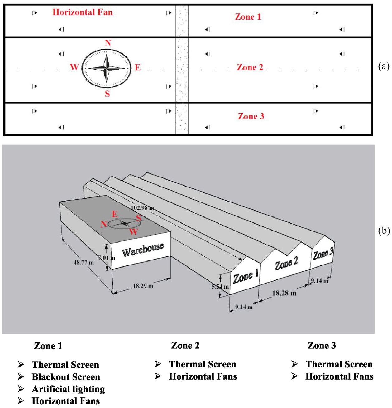
Schematic of case study greenhouse, dimensions, location of fans, and orientation.

Vapor mass balance

The humidity balance for a greenhouse is described by:

h \frac{d χ (t)}{dt} = E (t) - V (t) - D (t) - C (t)

(32)

E(t), C(t), D(t) and V(t) denote evapotranspiration (evaporation from plant’s leaves), condensation (on the greenhouse inside surfaces), dehumidification and ventilation respectively (per unit area of the greenhouse). It should be noted that since the relative humidity will be considered constant at 75%, the left-hand side of equation (32) is equal to 0.

$E (t)$ is calculated based on the Pennman–Monteith equation (Stanghellini and de Jong, 1995). In equation (33), $χ (t)$ is equal to relative humidity, 75%:

E (t) = \frac{2 LAI}{(1 + ε) r_{b} + r_{s}} [χ_{a i r, sat} (t) - χ (t) + \frac{ε r_{b}}{2 LAI} \frac{R_{n}}{L}]

(33)

C (t) = g_{c} [0.2522 e^{0.0485 T (t)} (T_{in} (t) - T_{out} (t)) - (χ_{air, sat} (t) - χ (t))]

(34)

V (t) = g_{v} (χ (t) - χ_{o} (t))

(35)

D (t) = g_{v, deh} (χ (t) - χ_{o} (t))

(36)

χ_{air, sat} (t) = 5.5638 e^{0.0572 T_{air}}

(37)

Where $g_{c}$ is calculated by equation (38) and g_v and g_v,deh are ventilation and dehumidification flow rates per unit area ( $m^{3} s^{- 1} . m^{- 2} \to m s^{- 1}$ ).

g_{C} = \max (0, 1.8 \times 10^{- 3} (T_{a} - T_{c}))^{\frac{1}{3}}

(38)

g_{v} = \frac{q_{vent} (t)}{A_{f}}

(39)

By using equations (1)−(39) and applying hourly climate data as well as the indoor humidity and temperature set points, the amount of hourly energy demand that is needed to maintain the desired temperature and relative humidity in the greenhouse is calculated. It is worthy to highlighted the point that since the selected greenhouse for this study is only using natural ventilation through roof ventilators, the values of $q_{Deh} (t)$ , $V (t)$ , $D (t)$ , $q_{vent} (t)$ , and $q_{ventMech} (t)$ are considered 0. However, this code is able to consider them for further studies.

Case study

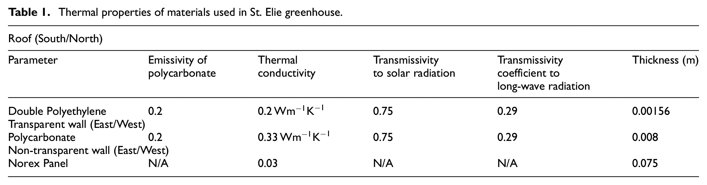
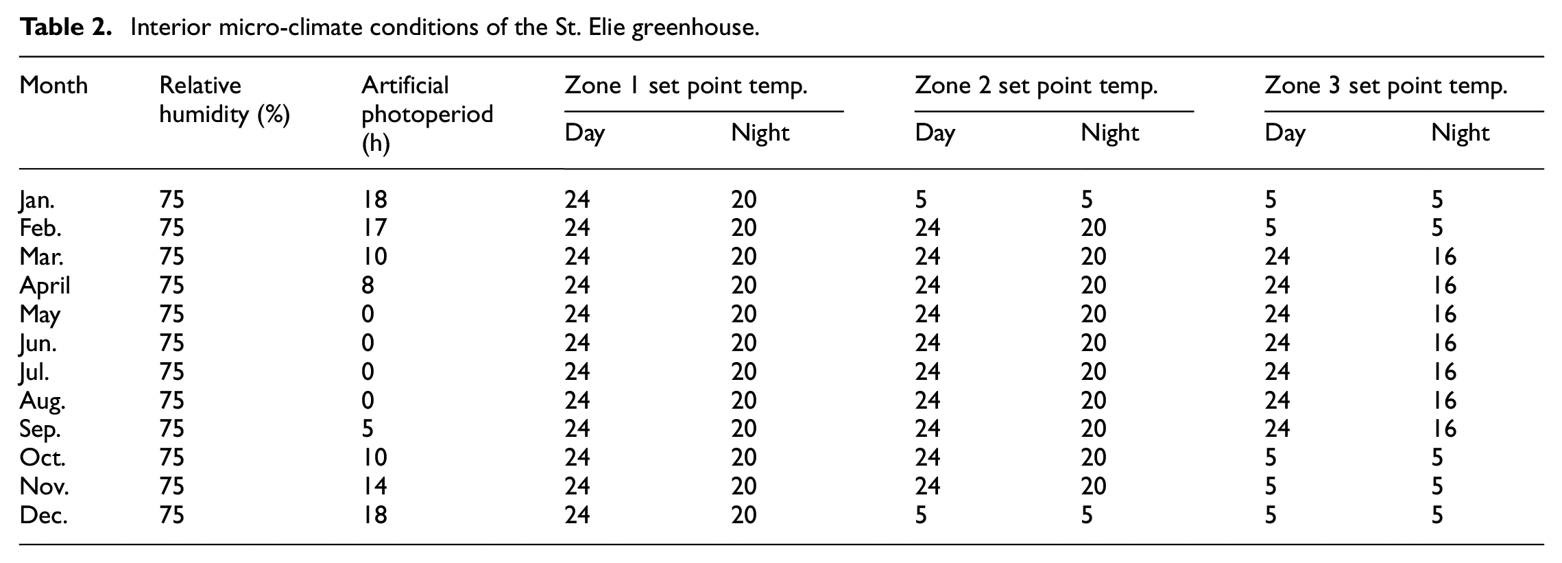
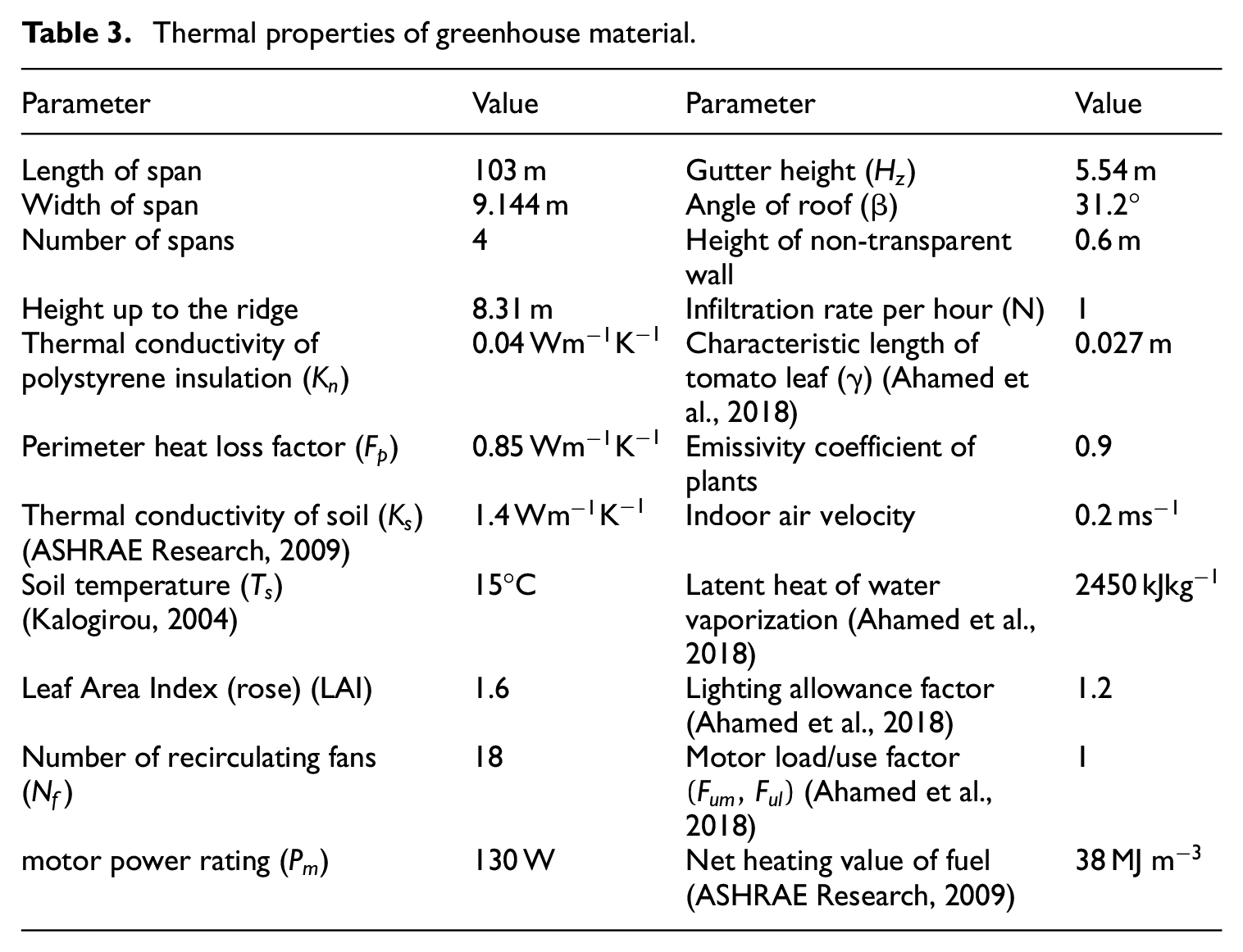
To validate the energy model accuracy, a flower greenhouse in the city of Sherbrooke, Quebec, Canada (45.4043° N, 71.8937° W) has been selected. This greenhouse, named “Les Serres St-Élie,” has three different micro-climate zones and a warehouse to support logistical requirements. Also, thermal screens, blackout screens and artificial lighting are employed in the greenhouse to reduce energy consumption and increase productivity. Each of the three zones has a different temperature and relative humidity setpoint for different months. Overall greenhouse dimensions and micro-climate conditions of the St. Elie greenhouse are illustrated in Tables 1 to 3, and Figure 3. These three zones are separated by vertical roll-up curtains. In this way, operators can merge or isolate the zones, as needed. To meet the energy demand, two natural gas boilers (Viessman CA3V- 3.0) with an output power of up to 879 kW each are installed in the greenhouse. To reduce temperature stratification and increase the air recirculation, 18 ceiling fans (model ECOfan+ CSA5400) are installed throughout the greenhouse (see Figure 3). To secure the maximum amount of productivity, artificial lighting equipment and horizontal blackout screens are installed in zone 1. All three zones have horizontal thermal screens. Table 2 lists the information concerning the artificial lighting for different months of the year.

Table 1.

Thermal properties of materials used in St. Elie greenhouse.

Roof (South/North)
Parameter	Emissivity of polycarbonate	Thermal conductivity	Transmissivity to solar radiation	Transmissivity coefficient to long-wave radiation	Thickness (m)
Double Polyethylene	0.2	0.2 W $m^{- 1} K^{- 1}$	0.75	0.29	0.00156
Transparent wall (East/West)
Polycarbonate	0.2	0.33 W $m^{- 1} K^{- 1}$	0.75	0.29	0.008
Non-transparent wall (East/West)
Norex Panel	N/A	0.03	N/A	N/A	0.075

Table 2.

Interior micro-climate conditions of the St. Elie greenhouse.

Month	Relative humidity (%)	Artificial photoperiod (h)	Zone 1 set point temp.		Zone 2 set point temp.		Zone 3 set point temp.
Month	Relative humidity (%)	Artificial photoperiod (h)	Day	Night	Day	Night	Day	Night
Jan.	75	18	24	20	5	5	5	5
Feb.	75	17	24	20	24	20	5	5
Mar.	75	10	24	20	24	20	24	16
April	75	8	24	20	24	20	24	16
May	75	0	24	20	24	20	24	16
Jun.	75	0	24	20	24	20	24	16
Jul.	75	0	24	20	24	20	24	16
Aug.	75	0	24	20	24	20	24	16
Sep.	75	5	24	20	24	20	24	16
Oct.	75	10	24	20	24	20	5	5
Nov.	75	14	24	20	24	20	5	5
Dec.	75	18	24	20	5	5	5	5

Table 3.

Thermal properties of greenhouse material.

Parameter	Value	Parameter	Value
Length of span	103 m	Gutter height ( $H_{z}$ )	5.54 m
Width of span	9.144 m	Angle of roof (β)	31.2°
Number of spans	4	Height of non-transparent wall	0.6 m
Height up to the ridge	8.31 m	Infiltration rate per hour (N)	1
Thermal conductivity of polystyrene insulation ( $K_{n}$ )	0.04 W $m^{- 1} K^{- 1}$	Characteristic length of tomato leaf ( $γ$ ) (Ahamed et al., 2018)	0.027 m
Perimeter heat loss factor ( $F_{p}$ )	0.85 W $m^{- 1} K^{- 1}$	Emissivity coefficient of plants	0.9
Thermal conductivity of soil ( $K_{s}$ ) (ASHRAE Research, 2009)	1.4 W $m^{- 1} K^{- 1}$	Indoor air velocity	0.2 $m s^{- 1}$
Soil temperature ( $T_{s}$ ) (Kalogirou, 2004)	15°C	Latent heat of water vaporization (Ahamed et al., 2018)	2450 $kJk g^{- 1}$
Leaf Area Index (rose) (LAI)	1.6	Lighting allowance factor (Ahamed et al., 2018)	1.2
Number of recirculating fans ( $N_{f}$ )	18	Motor load/use factor $(F_{um}, F_{ul})$ (Ahamed et al., 2018)	1
motor power rating ( $P_{m}$ )	130 W	Net heating value of fuel (ASHRAE Research, 2009)	38 MJ $m^{- 3}$

Computer code description and validation

The first part of the modeling task was accomplished using custom MATLAB-SIMULINK code. The inputs to this code are physical properties (dimensions, thermal properties, orientation, etc.) and interior micro-climate conditions (temperature and relative humidity set points, artificial lighting and thermal screen schedules, etc.) of the St. Elie greenhouse as design parameters, and Sherbrooke meteorological data (outside temperature, relative humidity, global horizontal irradiance, and wind speed). Figure 4 shows typical meteorological year (TMY) data for Sherbrooke.

Figure 4.

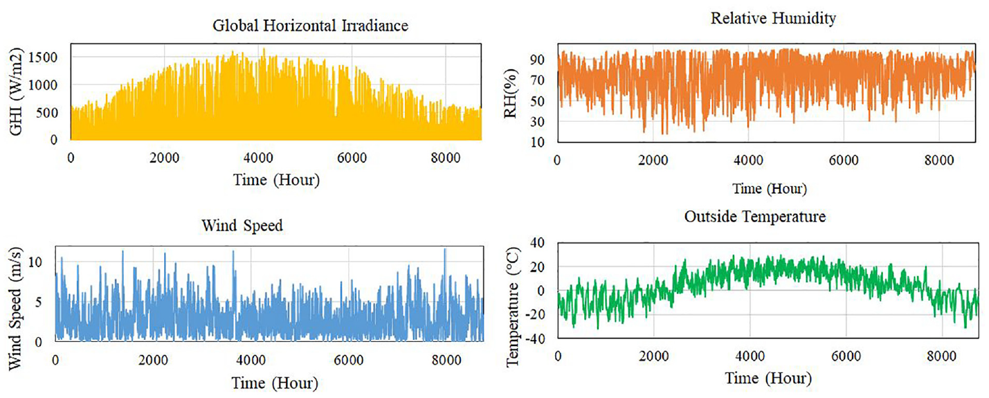
Local weather data of St. Elie greenhouse.

To verify the accuracy of the mathematical energy model, the actual and calculated energy consumption values of the St. Elie greenhouse are compared and depicted in Figure 5(a). The peak heating requirement occurred on February 3rd (with minimum temperature of −31.7 °C), which was 2.4% higher than the highest value in January (with minimum temperature of −30.5 °C). The results of the MATLAB code (MATLAB R2021b) show good agreement with energy consumption from St. Elie greenhouse, as extracted from the billing records for this period. The error of the developed MATLAB code for cold seasons, when the ventilation value is 0, is between 7% and 15%, which is acceptable. The early static energy model which were developed for greenhouse (Chiapale and Kittas, 1981; Morris, 1956) had accuracy of up to 25%, but this value for the recent dynamic models (Golzar et al., 2018; Singh R and Tiwari G, 2000) is around 11%. Weather data, and controlling strategy in greenhouse seems to have the highest contributions in generating errors.

Figure 5.

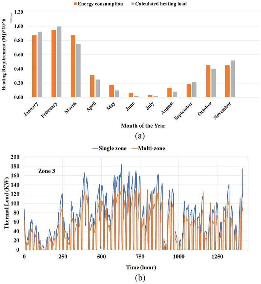
(a) Annual variation of the heating requirements in the St. Elie greenhouse versus heating load calculated by code and (b) the effect of multi-zone formulation on calculated heating load for January and February in zone 3.

Furthermore, it can be noticed that for the cold season, when the mechanical ventilation is off (i.e. roof vents and wall vents are closed) the model accuracy is maximum. In cold climate greenhouses, energy consumption is at its greatest during the cool/cold non summer months. Given that ventilation is principally required during the warm summer months, the simplifying assumption was made that the greenhouse has no ventilation system throughout the year. Although this assumption will introduce some error, particularly during the summer, it will provide valuable information concerning the potential for energy recovery within the greenhouse.

To present the importance of multi-zone formulation, Figure 5(b) compares the heating load in January and February for two formulations: single-zone and multi-zone, in zone 3. To do so, first the code ran for zone 3 as a single zone. It means four side of this zone exposed with outdoor temperature. The same process was repeated for multi-zone formulation but with one modification: north wall considered exposed with set point temperature of zone 2, and its relevant convection and convection heat transfer coefficient. As shown, in the multi-zone formulation the calculated heating demand for the cold season is less than that of the single-zone formulation. This demonstrates that a multi-zone formulation can bring higher accuracy than a simplified single-zone formulation in greenhouse simulation and design.

Results and discussion

As explained, the St Elie greenhouse has three distinct production zones and a warehouse, each with different micro-climate conditions. This fact causes each zone to have a different heating/cooling demand throughout the year, even in the summer season when the solar radiation is in its maximum value. Figure 6 presents the heating load of the three zones and the greenhouse warehouse.

Figure 6.

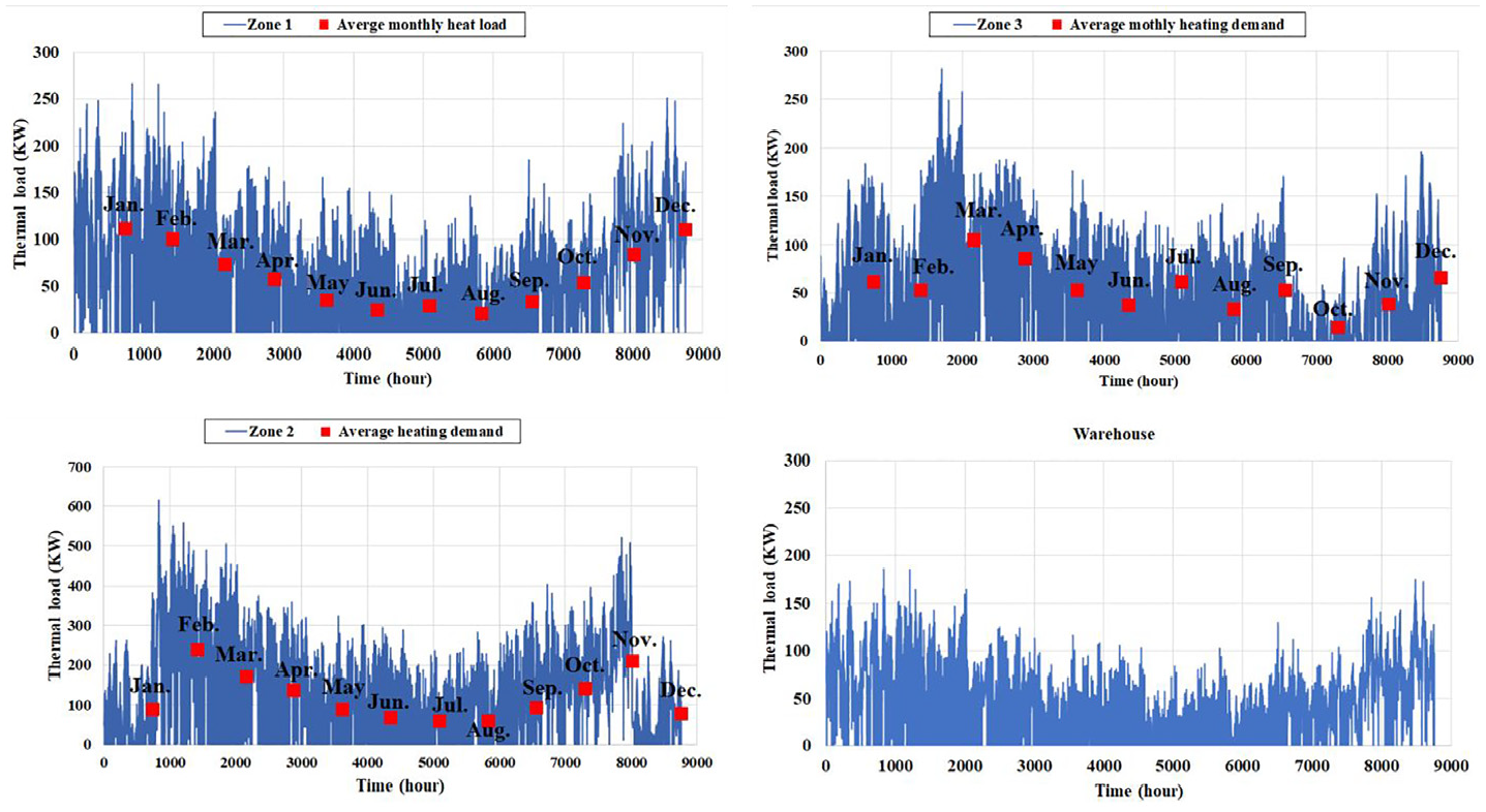
Heating demand of different zones of St. Elie greenhouse.

All commercial greenhouses have set points for temperature and relative humidity. These setpoints, as well as the target photoperiod, are presented in Table 2. The most convenient method to maintain the RH inside a greenhouse is natural ventilation through roof vents. However, while this method is the cheapest method, is also entails some disadvantages, especially in a cold agricultural region like Canada. It is reported that the dehumidification process by ventilation can cause up to 50% undesired heating load (Campen and Bot, 2001). Various studies (Kacira et al., 2004) have shown that there exists an optimum ratio (0.015–0.25) of the vent opening area to the ground area of a greenhouse to maximize the efficiency of natural ventilation. This ratio for St. Elie greenhouse is 0.21 when the roof vents are fully open. The main mechanism for natural ventilation is the existence of a pressure difference between the inside and the outside of the greenhouse. Parameters such as temperature, size, the location of the openings and wind speed can affect ventilation efficiency.

As part of this study, the dehumidification load of St. Elie greenhouse, as well as the contribution of different mechanisms involved in the water vapor balance of the indoor air were calculated. Figure 7(a) shows the total dehumidification load required to maintain the RH level of 75%. Figure 7(b) presents the contribution of different mechanisms involved in the water vapor balance of the indoor air: evapotranspiration, condensation, and infiltration (equation (32)). 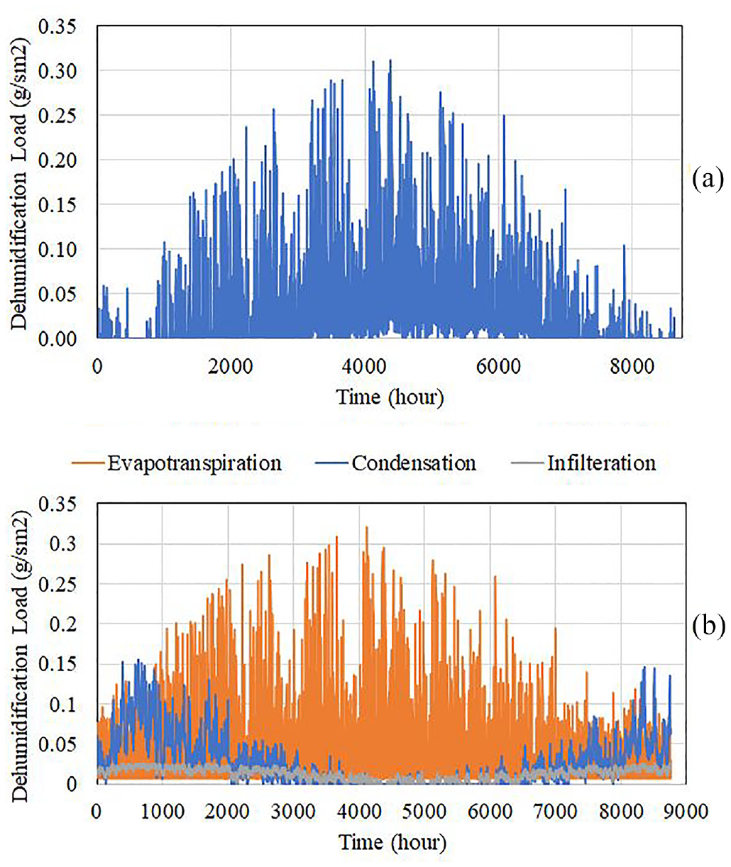Also, it should be highlighted that $V (t)$ in this study is considered 0. Figure 7 reveals that in the coldest period of year the dehumidification load is minimum. As a consequence, the roof ventilation system can be kept closed, which causes a reduction in energy consumption. Based on Figure 7(b), when the cover temperature falls below the dew point for the greenhouse, the condensation on the inside roof cover significantly reduces the need for dehumidification.

Figure 7.

Hourly distribution of (a) dehumidification load and (b) contribution of different mechanisms affecting the humidity level.

Energy saving strategies

Heat recovery

To reduce the greenhouse energy consumption, different strategies can be implemented. Figure 8 shows the cooling demand of zones 2 and 3 for the month of January in the St. Elie greenhouse. As shown in Table 2, the set point temperature and relative humidity of these zones are 5°C and 75%, respectively. The classic method of satisfying the cooling demand in a commercial greenhouse is by means of mechanical ventilation. This means that the roof ventilators, through the intervention of a control system, are sensitive to the greenhouse inside humidity and temperature. As soon as the measured parameter passes the set point, the control system opens the ventilators. However, based on Figure 8(b), during the coldest period of year (typical day Jan.16), it is possible to transfer hot air from zone 2 to zone 3, since zone 2 needs to remove hot air, while zone 3 requires heating. Our study on the St. Elie greenhouse shows that by installing a HRV (Heat Recovery Ventilator) between these two zones or by partially opening the roll-up separator between these two zones, for January and December, when the setpoint temperature is 5°C for both zones, there is an opportunity to cut the energy consumption up to 4.69% for January and 4.13% for December.

Figure 8.

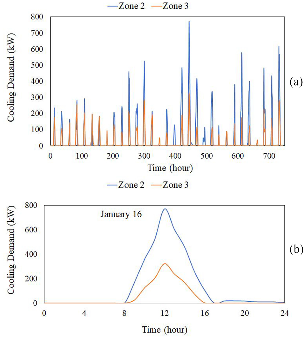
(a) variation of cooling demand $W m^{- 2}$ in zones 2 and 3 and (b) potential heat recovery in a typical day of January.

There is another opportunity to take advantage of heat recovery between zone 1 and zone 3. Based on Table 1 and Figure 6, during December and January the set point temperatures for zones 1 and 3 are 24°C and 5°C in the morning and 18°C and 5°C at night, respectively. Investigating the hourly heating/cooling load which is calculated by mathematical code shows that it is possible to transfer the hot air of zone 1 ( $T_{air} > 24 C^{°}$ ) to zone 2 in December and January, and to zone 3 in October, November, December, and January. The calculations for the month of January reveal that it is possible to meet 7% percent of the heating load of zone 3 by transferring the cooling demand from zone 1. It should be pointed out that there is a miss-match between the cooling time of zone 1 and the heating time of zone 2 or 3. To successfully accomplish the heat recovery process, some kind of energy storage equipment (Phase Change Material or hot water buffer tank) would be required. Figure 8 shows the cooling/heating demand of zones for a typical day (January 31). In this figure, the positive values represent heating demand, while negative ones show cooling demand. The area between the heating/cooling demand curve (where it has a negative value) and the abscissa corresponds to a potential heat recovery application.

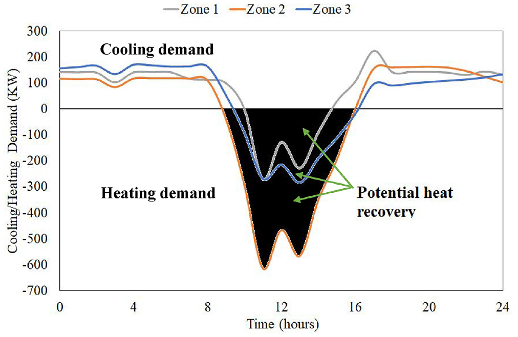
As can be seen in Figure 9, the black area related to zone 1 corresponds to warm air that is at or above the set point of zone 1 ( $24 C^{°}$ ); the associated heat can be stored and later released to zones 1, 2, or 3. Calculations show that the stored energy of zone 1 can meets 32% and 30% of the energy demand of zones 2 and 3, respectively. Also, considering the orange curve for zone 2, and the black area related to this curve, it can be seen that installing heat storage materials, whether within the north wall (Chinese style greenhouse) or Phase Change Material (PCH), can cut the energy cost up to 63% for the cold months when the set point temperature of zones 2 and 3 is 5°C.

Figure 9.

Heating and cooling demand for the St. Elie greenhouse zones 1, 2, and 3.

Having discussed heat recovery opportunities, it would also be worthwhile to consider how some parameters can affect the energy performance of a greenhouse: Orientation, geometrical properties, material, etc.

Solar radiation

It is proved that every parameter that can affect the greenhouse radiation efficiency (absorbed radiation by the greenhouse envelope/total radiation) can affect its energy performance (Esmaeli and Roshandel, 2020). If we consider a greenhouse as a solar collector, the orientation, area, roof angle, and construction material are the parameters that can affect its radiation performance. Figure 10 shows the hourly solar intensity on the different walls and roofs of the most southern portion (zone 3) of the St. Elie greenhouse for a typical day in summer and in winter. As can be seen, during winter there is less solar irradiance than during the summer. The south roof and south wall receive the highest amount of solar energy throughout the year. 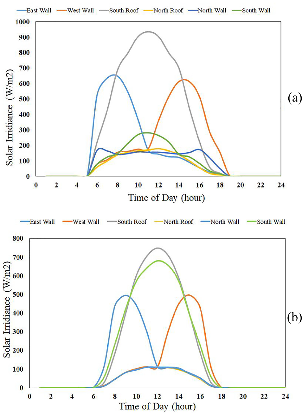However, in the winter season, the south wall receives more solar energy (+800 $W m^{- 2}$ ) in comparison with a summer day (+250 $W m^{- 2}$ ). So, based on this graph, it is recommended that the biggest transparent surface or face of a northern hemisphere greenhouse should be directed to the south. Further, it is recommended to insulate the north side of a northern hemisphere cold climate greenhouse since this side has the lowest contribution in heat gain by solar radiation phenomena. As depicted in Figure 2, in the St. Elie greenhouse, a warehouse is situated on the north side, which can play the role of insulation for the north side.

Figure 10.

Hourly variation of the total solar irradiance on different walls and roofs of the case study greenhouse: (a) in a typical day in summer and (b) in a typical day in winter.

As illustrated in Figure 10, the “South Roof,” meaning the sum of all south facing roof portions of the entire greenhouse, makes the greatest contribution to the greenhouse solar energy gain, even more than the south-facing wall. Based on this fact, different configurations can be proposed. For instance, an asymmetrical roof configuration is only one of the possible greenhouse configurations of interest. Esmaeli and Roshandel (2020) conducted a mathematical multi-functional optimization to design a Chinese style greenhouse with a minimum energy demand. Our study proposes a similar study in the future.

Figure 11, shows both symmetrical and asymmetrical roof configurations. The results and literature review show that increasing the area of the south wall, while the volume of greenhouse is constant, can affect the greenhouse energy consumption. However, obtaining the optimal geometrical parameters of such a configuration needs further study.

Figure 11.

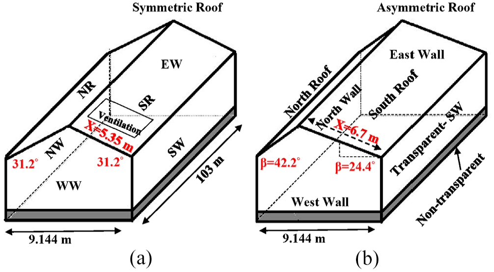
Isometric view of proposed configuration for St. Elie greenhouse (zone 3). (a) Symmetric roof and (b) asymmetric roof.

Obtaining the effect of an asymmetrical roof configuration on energy consumption of a greenhouse in a cold climate area requires a full CFD simulation, however, increasing the south roof area can affect the solar energy gain. In Figure 11, the values of X and β are 5.35 m and 31.2° for the actual symmetric roof, and 6.7 m and 24.4° for a hypothetical asymmetric roof, respectively. In this simplified evaluation, the greenhouse height, material (thermal properties), and micro-climate condition of greenhouse (temperature and relative humidity set point) remained unchanged. 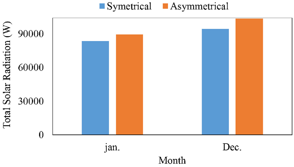Figure 12 shows and compares the available total solar irradiance ( $q_{solar}$ ) for symmetrical and asymmetrical roof configurations (Figure 11) for the St. Elie greenhouse (zone 3). As can be seen, the asymmetrical configuration receives around 5.5% greater solar radiation. Hence, based on this result, for a northern latitude, such as the St. Elie greenhouse in this study, or more generally for cold climate regions, it is recommended to design greenhouses in such a way that they can gain the highest solar radiation in the winter and summer. For the future study, it is proposed to do a multi objective optimization to find the best value for β and X.

Figure 12.

Variation in total solar irradiance availability in January and December in the St. Elie region (45°N) for two different roof configurations.

The orientation of a greenhouse can also affect its energy consumption. To evaluate the relative importance of greenhouse orientation, a simulation was conducted wherein the greenhouse was rotated 90 degrees to the east, while maintaining the warehouse on the north wall. Our results showed that the current east-west orientation has 2.67% less energy consumption, in comparison with a north-south orientation. Based on Figure 13, for the coldest months in a year, like January, February, and December, solar radiation in an east-west oriented greenhouse is higher than that of a north-south orientation, while for the hot months it is the reverse.

Figure 13.

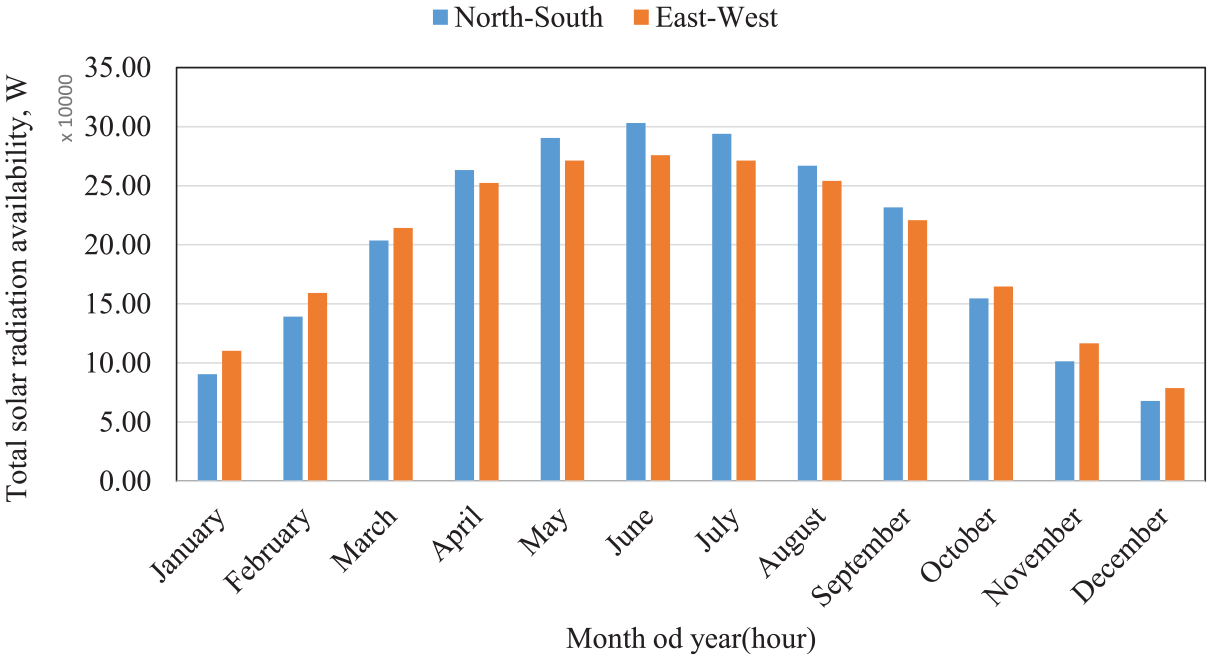
Comparison of annual variation in total solar irradiance availability for even-span greenhouse in E-W and N-S orientation for the St Elie greenhouse.

A thermal screen, also known as an energy screen, shading screen, or thermal curtain, is an important component in modern greenhouse technology. It is used to help control and manage the micro-climate within a greenhouse by regulating the amount of sunlight and heat that enters or exits the structure; it can help regulate the internal temperature of the greenhouse. Note that one says that a thermal screen, or curtain, is open, when one can see the sky; it is closed when the sky is hidden. At night during cold weather, the thermal screens can be closed to retain heat within the greenhouse by reducing thermal loses to the cold night sky. They can block excessive sunlight during hot days, reducing the greenhouse temperature, especially during the summer. Greenhouses adopt a control strategy to activate the artificial lighting and thermal screens. Usually, artificial lighting, blackout screens, and thermal screens are controlled by means of a combination of a timing schedule and the solar radiation level. In our study, when the radiation level is less than 50 W/m², the thermal screens are activated (i.e. closed). Also in zone 1, when artificial lighting is on, the blackout screens are activated. The schedule of artificial lighting is provided in Table 2.

Figure 14 shows and compares the heating demand of zone 3 of the St. Elie greenhouse in January, both with and without the use of thermal screens. The calculations confirmed that using a thermal screen can reduce the energy demand by as much as 20% for zone 3 in January.

Figure 14.

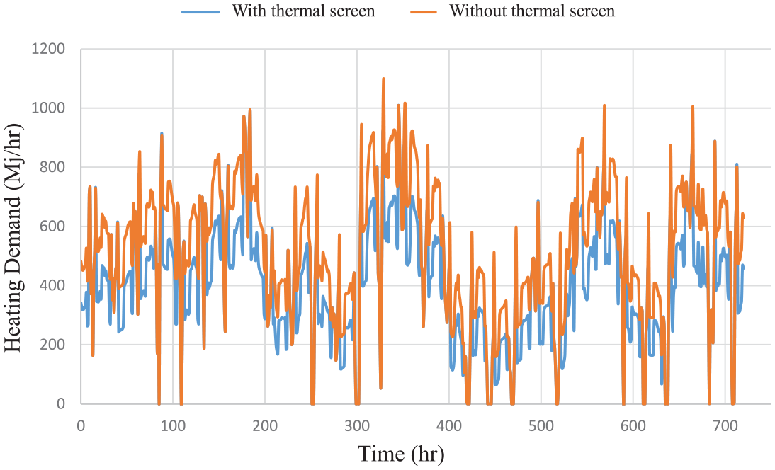
Comparison of heating demand of zone 3 in January with and without thermal screen.

Conclusion

This study presented a mathematical energy model capable of calculating the heating, cooling and dehumidification loads of a multi-zone (i.e. multiple micro-climate) greenhouse. The development of the model is based on simultaneous energy and vapor mass balances. The resulting MATLAB-Simulink code was then used to investigate potential solutions for reducing the energy consumption in multi-zone greenhouses in cold climate agricultural regions, such as found in Quebec, Canada. As a case study, a greenhouse in Sherbrooke, Quebec, named Les Serres St-Élie, was selected. It covers more than 5000 $m^{2}$ and is equipped with thermal screens, a blackout screen, artificial lighting, and can have different temperature set points and humidity setpoints in each of its three micro-climate zones. The results showed that the accuracy of this model is within 15% of the actual energy consumption. It was demonstrated that a heat storage strategy with Phase Change materials leads to a reduction in energy consumption in a typical day. The total amount of solar radiation over different surfaces was calculated. The maximum solar radiation heat gain is due to the south roof and the east/west wall in summer, and to the south roof and the south wall in winter. Based on this study, it is best to build cold climate greenhouses in an east-west direction. Also, increasing the area of the south roof for northern hemisphere greenhouses is a possible solution to maximizing the total amount of solar energy gain in cold regions. Consequently, an asymmetrical roof configuration is proposed in such cases. However, to obtain the exact dimensions, an optimization study is necessary.

Footnotes

Appendix

Table 4.

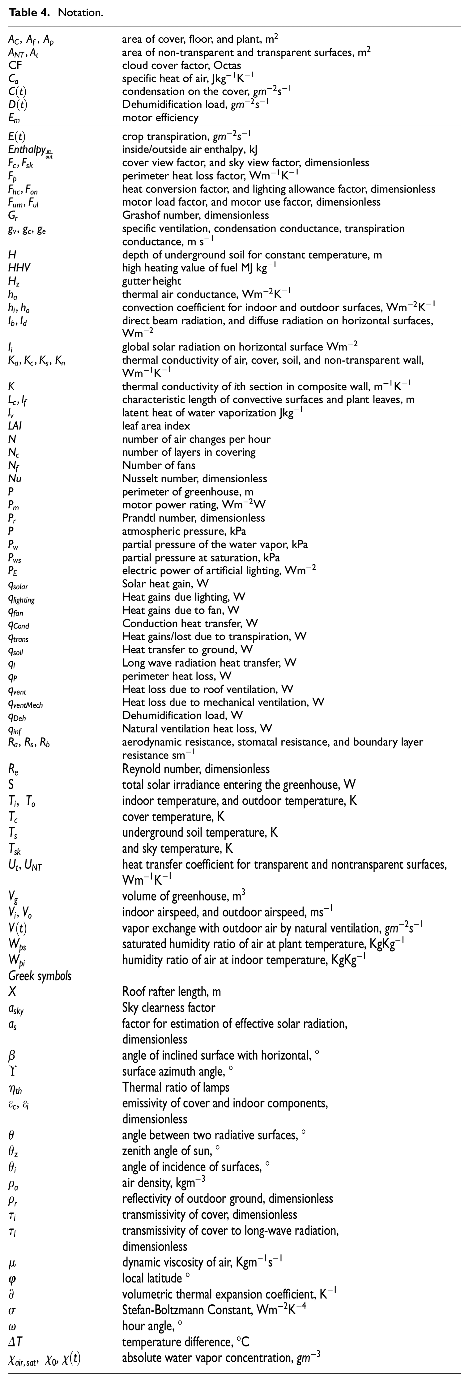
Notation.

$A_{C}, A_{f}, A_{p}$	area of cover, floor, and plant, $m^{2}$
$A_{NT}, A_{t}$	area of non-transparent and transparent surfaces, $m^{2}$
CF	cloud cover factor, Octas
$C_{a}$	specific heat of air, $Jk g^{- 1} K^{- 1}$
$C (t)$	condensation on the cover, $g m^{- 2} s^{- 1}$
$D (t)$	Dehumidification load, $g m^{- 2} s^{- 1}$
$E_{m}$	motor efficiency
$E (t)$	crop transpiration, $g m^{- 2} s^{- 1}$
$Enthalp y_{\frac{in}{out}}$	inside/outside $air enthalpy$ , kJ
$F_{c}, F_{sk}$	cover view factor, and sky view factor, dimensionless
$F_{p}$	perimeter heat loss factor, W $m^{- 1} K^{- 1}$
$F_{h c}, F_{o n}$	heat conversion factor, and lighting allowance factor, dimensionless
$F_{um}, F_{ul}$	motor load factor, and motor use factor, dimensionless
$G_{r}$	Grashof number, dimensionless
$g_{v}$ , $g_{c}$ , $g_{e}$	specific ventilation, condensation conductance, transpiration conductance, m $s^{- 1}$
H	depth of underground soil for constant temperature, m
HHV	high heating value of fuel MJ $k g^{- 1}$
$H_{z}$	$gutter height$
$h_{a}$	thermal air conductance, W $m^{- 2} K^{- 1}$
$h_{i}, h_{o}$	convection coefficient for indoor and outdoor surfaces, W $m^{- 2} K^{- 1}$
$I_{b}, I_{d}$	direct beam radiation, and diffuse radiation on horizontal surfaces, W $m^{- 2}$
$I_{i}$	global solar radiation on horizontal surface W $m^{- 2}$
$K_{a}, K_{c}, K_{s}$ , $K_{n}$	thermal conductivity of air, cover, soil, and non-transparent wall, W $m^{- 1} K^{- 1}$
K	thermal conductivity of ith section in composite wall, $m^{- 1} K^{- 1}$
$L_{c}, l_{f}$	characteristic length of convective surfaces and plant leaves, m
$l_{v}$	latent heat of water vaporization J $k g^{- 1}$
LAI	leaf area index
N	number of air changes per hour
$N_{c}$	number of layers in covering
$N_{f}$	Number of fans
Nu	Nusselt number, dimensionless
P	perimeter of greenhouse, m
$P_{m}$	motor power rating, $W m^{- 2}$ W
$P_{r}$	Prandtl number, dimensionless
P	atmospheric pressure, kPa
$P_{w}$	partial pressure of the water vapor, kPa
$P_{ws}$	partial pressure at saturation, kPa
$P_{E}$	electric power of artificial lighting, $W m^{- 2}$
$q_{solar}$	Solar heat gain, W
$q_{lighting}$	Heat gains due lighting, W
$q_{fan}$	Heat gains due to fan, W
$q_{Cond}$	Conduction heat transfer, W
$q_{trans}$	Heat gains/lost due to transpiration, W
$q_{soil}$	Heat transfer to ground, W
$q_{l}$	Long wave radiation heat transfer, W
$q_{P}$	perimeter heat loss, W
$q_{vent}$	Heat loss due to roof ventilation, W
$q_{ventMech}$	Heat loss due to mechanical ventilation, W
$q_{Deh}$	Dehumidification load, W
$q_{\inf}$	Natural ventilation heat loss, W
$R_{a}$ , $R_{s}$ , $R_{b}$	aerodynamic resistance, stomatal resistance, and boundary layer resistance $s m^{- 1}$
$R_{e}$	Reynold number, dimensionless
S	total solar irradiance entering the greenhouse, W
$T_{i}$ , $T_{o}$	indoor temperature, and outdoor temperature, K
$T_{c}$	cover temperature, K
$T_{s}$	underground soil temperature, K
$T_{sk}$	and sky temperature, K
$U_{t}$ , $U_{NT}$	heat transfer coefficient for transparent and nontransparent surfaces, W $m^{- 1} K^{- 1}$
$V_{g}$	volume of greenhouse, $m^{3}$
$V_{i}$ , $V_{o}$	indoor airspeed, and outdoor airspeed, $m s^{- 1}$
$V (t)$	vapor exchange with outdoor air by natural ventilation, $g m^{- 2} s^{- 1}$
$W_{ps}$	saturated humidity ratio of air at plant temperature, Kg $K g^{- 1}$
$W_{pi}$	humidity ratio of air at indoor temperature, Kg $K g^{- 1}$
Greek symbols
X	Roof rafter length, m
$a_{sky}$	Sky clearness factor
$a_{s}$	factor for estimation of effective solar radiation,dimensionless
$β$	angle of inclined surface with horizontal, °
ϒ	surface azimuth angle, °
η _th	Thermal ratio of lamps
$ε_{c}$ , $ε_{i}$	emissivity of cover and indoor components,dimensionless
$θ$	angle between two radiative surfaces, °
$θ_{z}$	zenith angle of sun, °
$θ_{i}$	angle of incidence of surfaces, °
$ρ_{a}$	air density, $kg m^{- 3}$
$ρ_{r}$	reflectivity of outdoor ground, dimensionless
$τ_{i}$	transmissivity of cover, dimensionless
$τ_{l}$	transmissivity of cover to long-wave radiation,dimensionless
μ	dynamic viscosity of air, $Kg m^{- 1} s^{- 1}$
φ	local latitude °
∂	volumetric thermal expansion coefficient, $K^{- 1}$
σ	Stefan-Boltzmann Constant, W $m^{- 2} K^{- 4}$
ω	hour angle, °
ΔT	temperature difference, °C
$χ_{air, sat}$ , $χ_{0}$ , $χ (t)$	absolute water vapor concentration, $g m^{- 3}$

Credit author statement

Hosein Faramarzpour: Conceptualization, Methodology, Investigation, Validation, Software, Visualization, Writing - original draft, Writing - review & editing. Mohsen Ghaderi: Conceptualization, Software, Methodology. Christopher Reddick: Conceptualization, Validation, Writing - review & editing. Michel Grégoire: Validation, Funding. Mikhail Sorin: Methodology, Writing - review & editing Supervision, Resources, Methodology, Funding acquisition, Writing - review & editing.

Declaration of conflicting interests

The author(s) declared no potential conflicts of interest with respect to the research, authorship, and/or publication of this article.

Funding

The author(s) disclosed receipt of the following financial support for the research, authorship, and/or publication of this article: The authors acknowledge the financial support of the Natural Sciences and Engineering Research Council of Canada for this project (RGPIN-2019-05826).

ORCID iD

Hosein Faramarzpour

References

Ahamed

Guo

Tanino

(2018) A quasi-steady state model for predicting the heating requirements of conventional greenhouses in cold regions. Information Processing in Agriculture 5(1): 33–46.

Ahamed

Guo

Tanino

(2020) Modeling heating demands in a Chinese-style solar greenhouse using the transient building energy simulation model TRNSYS. Journal of Building Engineering 29: 101114.

Ahamed

Guo

Taylor

, et al. (2019) Heating demand and economic feasibility analysis for year-round vegetable production in Canadian prairies greenhouses. Information Processing in Agriculture 6(1): 81–90.

Al-Ismaili

Jayasuriya

(2016) Seawater greenhouse in Oman: A sustainable technique for freshwater conservation and production. Renewable and Sustainable Energy Reviews 54: 653–664.

ASHRAE Research (2009) ASHRAE® Handbook-Fundamentals. New York: American society of Heating, Refrigerating and Air-Conditioning Engineers.

Barbosa

Gadelha

Kublik

, et al. (2015) Comparison of land, water, and energy requirements of lettuce grown using hydroponic vs conventional agricultural methods. International Journal of Environmental Research and Public Health 12(6): 6879–6891.

Beshada

Zhang

Boris

(2006) Winter performance of a solar energy greenhouse in southern Manitoba. Canadian Biosystems Engineering 48(5): 1–8.

Bot

(1988) Greenhouse simulation models. Engineering and Economic Aspects of Energy Saving in Protected Cultivation 245: 315–325.

Campen

Bot

(2001) SE—Structures and Environment: Design of a low-energy dehumidifying system for greenhouses. Journal of Agricultural Engineering Research 78(1): 65–73.

10.

Chen

, et al. (2018) A computational model to determine the optimal orientation for solar greenhouses located at different latitudes in China. Solar Energy 165: 19–26.

11.

Chen

Zhao

, et al. (2015) Modeling of energy demand in the greenhouse using PSO-GA hybrid algorithms. Mathematical Problems in Engineering 2015: 1–6.

12.

Chiapale

Kittas

(1981) Estimation regionale des besoins de chauffage des serres. Acta Hortic, 115: 493–503.

13.

Clark

Allen

(1978) The estimation of atmospheric radiation for clear and cloudy skies. In: Proc. 2nd national passive solar conference (AS/ISES), Newark, Del.: American Section of the International Solar Energy Society. 1978, pp.675–678.

14.

De Zwart

(1996) Analyzing energy-saving options in greenhouse cultivation using a simulation model, Thesis, Wageningen University and Research.

15.

Duffie

Beckman

(2013) Solar Engineering of Thermal Processes. Hoboken, NY: John Wiley & Sons.

16.

Esmaeli

Roshandel

(2020) Optimal design for solar greenhouses based on climate conditions. Renewable Energy 145: 1255–1265.

17.

Gao

L-H

Ren

H-Z

, et al. (2010) Structure, function, application, and ecological benefit of a single-slope, energy-efficient solar greenhouse in China. HortTechnology 20(3): 626–631.

18.

Ghaderi

Hosseinnia

Sorin

(2023) Assessment of waste heat recovery potential in greenhouse ventilation systems using dynamic pinch analysis. Applied Thermal Engineering 227: 120363.

19.

Ghani

Bakochristou

ElBialy

EMAA

, et al. (2019) Design challenges of agricultural greenhouses in hot and arid environments – A review. Engineering in Agriculture Environment and Food 12(1): 48–70.

20.

Golzar

Heeren

Hellweg

, et al. (2018) A novel integrated framework to evaluate greenhouse energy demand and crop yield production. Renewable and Sustainable Energy Reviews 96: 487–501.

21.

Kacira

Sase

Okushima

(2004) Effects of side vents and span numbers on wind-induced natural ventilation of a gothic multi-span greenhouse. Japan Agricultural Research Quarterly 38(4): 227–233.

22.

Kalogirou

Florides

(2004) Measurements of ground temperature at various depths. Kanazawa, Japan: Cyprus University of Technology.

23.

Liu

Jordan

(1961) Daily insolation on surfaces tilted towards equator. ASHRAE Transactions 3: 53–53.

24.

Liu

BYH

Jordan

(1963) The long-term average performance of flat-plate solar-energy collectors: With design data for the US, its outlying possessions and Canada. Solar Energy 7(2): 53–74.

25.

Luo

Feije

Zwart

Dail

, et al. (2005) Simulation of greenhouse management in the subtropics, Part I: Model validation and scenario study for the winter season. Biosystems Engineering 90(3): 307–318.

26.

Mohammadi

Ranjbar

Ajabshirchi

(2018) Application of dynamic model to predict some inside environment variables in a semi-solar greenhouse. Information Processing in Agriculture 5(2): 279–288.

27.

Morris

(1956) Some aspects of the control of plant environment. Journal of Agricultural Engineering Research 1: 156–66.

28.

Singh

Tiwari

(2000) Thermal heating of controlled environment greenhouse: a transient analysis. Energy conversion and management 41(5): 505–522.

29.

Stanghellini

de Jong

(1995) A model of humidity and its applications in a greenhouse. Agricultural and Forest Meteorology 76(2): 129–148.

30.

Takakura

(1993) Climate Under Cover: Digital Dynamic Simulation in Plant Bio-Engineering. Kanazawa, Japan: Springer.

31.

Tong

Christopher

, et al. (2013) Passive solar energy utilization: A review of cross-section building parameter selection for Chinese solar greenhouses. Renewable and Sustainable Energy Reviews 26: 540–548.

32.

Trigui

Barrington

Gauthier

(2001) SE—Structures and environment: A strategy for greenhouse climate control, Part I: Model development. Journal of Agricultural Engineering Research 78(4): 407–413.

33.

Vadiee

(2011) Energy analysis of the closed greenhouse concept: Towards a sustainable energy pathway, KTH Royal Institute of Technology.

34.

Vadiee

Martin

(2014) Energy management strategies for commercial greenhouses. Applied Energy 114: 880–888.

35.

van’t Ooster

Van Henten

Janssen

, et al. (2007) Development of concepts for a zero-fossil-energy greenhouse. Acta Horticulturae 801: 725–732.

36.

Van Beveren

Bontsema

Van Straten

, et al. (2015) Minimal heating and cooling in a modern rose greenhouse. Applied Energy 137: 97–109.

37.

Zaragoza

Buchholz

Jochum

, et al. (2007) Watergy project: Towards a rational use of water in greenhouse agriculture and sustainable architecture. Desalination 211(1-3): 296–303.

38.

Zhang

Wang

Zou

, et al. (2016) CFD and weighted entropy based simulation and optimisation of Chinese Solar Greenhouse temperature distribution. Biosystems Engineering 142: 12–26.

Specification of a greenhouse in cold climate condition,mathematical model and optimization

Abstract

Keywords

Introduction

Model development

Energy balance

Vapor mass balance

Case study

Computer code description and validation

Results and discussion

Energy saving strategies

Heat recovery

Solar radiation

Conclusion

Footnotes

Appendix

Credit author statement

Declaration of conflicting interests

Funding

ORCID iD

References