Experimental method for estimating the effect of solar radiation on the inner surface heat flux of opaque building envelope elements

Abstract

There still exists a considerable difference when comparing the real and the design energy consumption of buildings. The difference between the design and the real building envelope energy performance is one of its main reasons. The building envelope can be characterised through the individual characterisation of its different building envelope components such as opaque walls or windows. Therefore, the estimation of parameters such as their transmission heat transfer coefficient (UA) and their solar aperture (gA) is usually implemented. Although building components have been analysed over the years, the thermal characteristics of buildings have mainly been estimated through steady-state laboratory tests and simplified calculation/simulation procedures based on theoretical data. The use of inverse modelling based on registered dynamic data has also been used; however, unfortunately, the models used tend to significantly simplify or neglect the solar radiation effect on the inner surface heat flux of opaque building envelope elements. Therefore, this work presents an experimental, dynamic and inverse modelling method that accurately models non-linear phenomena through the use of a user-friendly simulation programme (LORD). The method is able to analyse in detail the effect of the solar radiation on the inner surface heat flux of opaque building envelope elements, without the necessity of knowing their constructive details or thermal properties. The experiment is performed in a fully monitored test box, where different models are tested with different opaque walls to find the best fit. Finally, the solar irradiance signal is removed from the best models so as to accurately quantify the weight of the solar radiation on the inner surface heat flux of each wall for two extreme periods, one for sunny summer days and other for cloudy winter days.

Introduction

Energy efficiency was not considered a major issue when constructing buildings until the 1970s in the European Union (H2020 EeB, 2020). However, the European Union’s interest in the energy efficiency of buildings has increased over the last few years, as can be seen in the implemented directives (European Parliament, 2018). However, efficient buildings are not easily achieved. Nowadays, it is common to face such problems as inefficiency or the considerable difference between the design and real energy consumption values. The latter is commonly known as the performance gap (Salehi et al., 2015; Xu and Zou, 2020; Zou et al., 2018). Several factors, such as the behaviour of the users or the performance of the energy systems, can influence the resulting overall performance of the buildings. Moreover, the building envelope is one of the factors with a considerable impact on the performance gap (Johnston et al., 2015). The main performance characteristics of building envelopes are the Heat Loss Coefficient (HLC [W/K]) and the Solar Aperture (S_a or gA [m²]) (Housez et al., 2014). The HLC is the sum of the entire envelope’s transmission heat loss coefficient (UA value [W/K]) and the infiltration/ventilation heat loss coefficient (C_v [W/K]) (Kim et al., 2022). However, the building envelope’s solar aperture, as (Baker, 2015) explains, is ‘the heat flow rate transmitted through the building envelope to the internal environment under steady state conditions, caused by solar radiation incident at the outside surface, divided by the intensity of incident solar radiation’. Once this parameter has been obtained, it is possible to estimate the solar gains of a building, simply multiplying the solar aperture by the corresponding solar radiation incident on the wall or window.

The in-situ estimation of the Heat Loss Coefficient or the UA value has been widely studied through different approaches. Moreover, the fact that building envelope components, such as windows or opaque walls, absorb solar energy is also well known and studied. Although, in some cases, the solar gains through opaque walls are not considered in building envelope characterisations, there are several methods to estimate them for different building energy components. On the one hand, the ISO 52016-1 (ISO 52016-1, 2017) presents simplified characteristic values for the calculation of the solar heat gains that occur through opaque walls that can be used for building energy performance calculations. However, the ISO 52016-1 is based on theoretical calculations, using theoretical values of such parameters as the surface solar absorptivity of the analysed elements. Unfortunately, these theoretical parameters commonly show a considerable uncertainty, which would be directly transferred to the final estimate of solar heat gains. In order to avoid these uncertainties, methods based on real data could be used.

On the other hand, the characterisation of different building envelope components, such as opaque walls, based on real measured data, have also been studied using outdoor test cells. The PASSYS-PASLINK projects include some of the largest and best known (Strachan and Baker, 2008). All the activities, procedures and expertise developed in PASLINK have been continued and considered through the modelling and analysis in DYNamic Analysis, Simulation and Testing applied to the Energy and Environmental performance of buildings (DYNASTEE) platform, this being a group supported by INIVE (Bloem et al., 2020; Dynastee, 2021). Moreover, various PASLINK tests have been used by several authors for many kinds of analysis and are still being used for research, as evidenced by recent publications (Dimoudi et al., 2016; Martínez et al., 2019). In most cases, direct modelling (through simulation programmes based on theoretical data) has been used to model buildings’ thermal characteristics. However, inverse modelling methods (based on registered data) have also been applied. When using these models, it is important to verify the identifiability of the model structure before tackling the inverse problem. Furthermore, consideration should be given to the inclusion of approximation errors, conducting comprehensive residual analyses to diagnose any unaccounted phenomena, estimating confidence regions for the parameters and achieving an appropriate trade-off between model complexity and accuracy (Rouchier, 2018). However, these inverse models tend to be notably simplified (linear modelling). For example, within the PASLINK project, several authors have compared or analysed the ARMAX models, state-space models and RC models (Deconinck and Roels, 2017; Jiménez et al., 2008b; Strachan and Vandaele, 2008) applied to different building components where opaque walls can be found. Despite this, the majority of these works conclude that the use of non-linear models would provide more accurate results. Therefore, some authors have incorporated the non-linear effects on building components. For example, (Jiménez et al., 2008b) includes them in two different ways: considering them in a non-linear form using CTSM-R or linearising them using ARX models. Moreover, the works (Jiménez et al., 2008a; Naveros et al., 2014) include these non-linear effects on, respectively, photovoltaic modules or simple walls using CTSM-R. However, the inclusion of the non-linear effects in inverse modelling can be complicated and time-consuming, depending on the software used.

Beyond the purview of the PASLINK project, several research works have determined the thermal properties of building components. For example, (Iglesias et al., 2018) and (Demeyer et al., 2021) both propose approaches based on Bayesian inference and uncertainty analysis to estimate the thermal properties of walls. They use simplified heat transfer models and in-situ measurements of temperature and heat flux to establish the relationship with the unknown thermal properties. Furthermore, (Sassine et al., 2019) presents a method for determining the thermophysical properties of a building wall through in-situ measurements of temperature and heat flux using the inverse method. Experimental tests are conducted and compared with numerical results to identify the thermophysical parameters of the wall. Articles such as (Evangelisti et al., 2018) and (Ha et al., 2020) include methods where they work with experimental measurements and data obtained by numerical simulations, respectively. Nevertheless, these studies confine their scope to analysing the method, focussing on the assessment of model quality and uncertainty quantification, while failing to propose any additional analysis beyond that. In other words, the majority use simplified models to estimate such thermal parameters as resistances and capacitances.

Furthermore, the International Energy Agency IEA-EBC programme (IEA-EBC Annex 58, 2020) Annex 58, titled ‘Reliable building energy performance characterisation based on full scale dynamic measurements’, has also continued to work with building envelope component analysis based on real measured data. The Round Robin Box test (Jiménez, 2016) is one of the activities carried out by the Annex 58 project (see Figure 1). In general, the researchers analysing the opaque walls of this box only focus on the estimation of the U-value and g-value. Moreover, in (Chávez et al., 2019), no improvement is found in the U-value estimation when the solar irradiance is included in the models. However, as far as the authors know, no one has carried out a deeper analysis of the solar radiation effect on inner surface heat flux. If the said flux is analysed, it is possible to quantify the inner surface heat flux blocked (by the incident solar radiation heating the outer surface) from going to the exterior.

Figure 1.

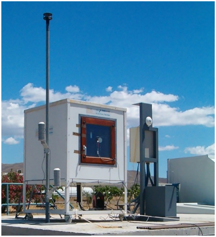
The test box during its experiment in Almeria.

Therefore, this paper proposes an innovative experimental inverse modelling method for the analysis of the effect of the corresponding incident solar radiation affecting the inner surface heat flux of each of the opaque faces of the abovementioned Round Robin Experiment box. The main difference of this method from the most commonly used building components analysis methods is that it analyses the effect of the solar radiation on the inner surface heat flux based on the use of real in-situ measured data. In other words, this novel dynamic method relies on an inverse modelling procedure that can accurately model a wall without the necessity of knowing the properties of the wall’s construction materials. Then, using only the measured inner surface heat flux, the surface temperatures of both sides of the walls and the ambient or weather conditions; it is possible to accurately estimate the solar radiation effect on the inner surface heat flux. In order to test this, each opaque face of the box is analysed one by one, considering how the solar radiation is affecting each of the inner surface heat flux measurements. Since the box was monitored in detail, it has been possible to obtain a very detailed dataset for each of the faces. This experimental inverse modelling method is based on RC models, using the user-friendly LORD software (Gutschker, 2003; Gutschker, 2008). Due to its simplicity, it is easy to test linear models where non-linear effects, such as the effects of wind speed and long wave radiation, are also included. During the analysis of the opaque walls of the Round Robin Box, two very extreme periods have been tested. The experimental periods were chosen in order to assess the effect of the solar radiation on the inner surface heat flux and its variability under very different extreme conditions: a summer period with high levels of solar radiation and a cloudy period in winter with very low solar radiation. Within the available data, the longest possible sunny and cloudy periods were selected. This, as far as the authors’ knowledge, has never been done before with this exactness using the LORD software.

Materials: Round Robin Box

Description of the Round Robin Box

The proposed analysis is carried out in the Round Robin Box that represents a building in miniature. It was constructed in the framework of the IEA EBC Annex 58 by KU Leuven and gave support to several research activities conducted in the framework of this Annex, including a series of tests producing data used in that framework and available for further research (Jiménez, 2016).

The test box has an exterior volume of 120 × 120 × 120 cm³ and all the walls, floor and ceiling have the same thickness of 12 cm. Thus, the dimensions of the inner surface of the Round Robin Box are 96 × 96 × 96 cm³. There is a wooden window of 71 × 71 cm² located in one side of the box with a glazed part of 52 × 52 cm². Moreover, the Round Robin Box is not in contact with the floor in order to avoid the effects of the ground on the box’s behaviour. The test box can be seen in Figure 1, located in CIEMAT’s Plataforma Solar de Almería (Spain). Figure 2 shows the material properties of the box layers.

Figure 2.

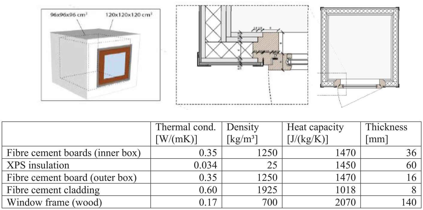
Schematic view of the design of the round robin test box and material properties of the different layers of the box as provided by the manufacturer presented by KU Leuven in Jiménez (2016).

Input data

The Round Robin Box experiment has been carried out in several locations in Europe within the framework of the IEA EBC Annex 58. However, only the data regarding the tests carried out at CIEMAT’s Solar Platform in Tabernas (lat. 37.09°, long. −2.35°), Almeria (Spain), have been analysed during this study, due to the availability of multiple extra sensors included in the experimental set up. Moreover, Almeria receives a high solar radiation during both summer and winter, so the obtained solar irradiance measurements are very useful for carrying out the proposed study.

The experiment in Almeria was conducted over eight months; including a first period under summer conditions and a second period under winter conditions. The summer dataset considers the period from 31st May 2013 to 2nd July 2013. In this period, two different tests were performed: constant indoor air temperature set point (at 40°C) and a Randomly Ordered Logarithmic Binary Sequence (ROLBS) power sequence (Van Dijk and Van der Linden, 1993). The winter dataset considers the period from 6th December 2013 to 7th January 2014. In this period, three different tests were performed: two co-heatings with constant indoor air temperature set point (one at 35°C and the second at 21°C) and a ROLBS power sequence. Then, once both datasets had been individually analysed by plotting each of the measured data and visually checking them to find any irregularities, summer and winter datasets were divided into shorter periods for analysis.

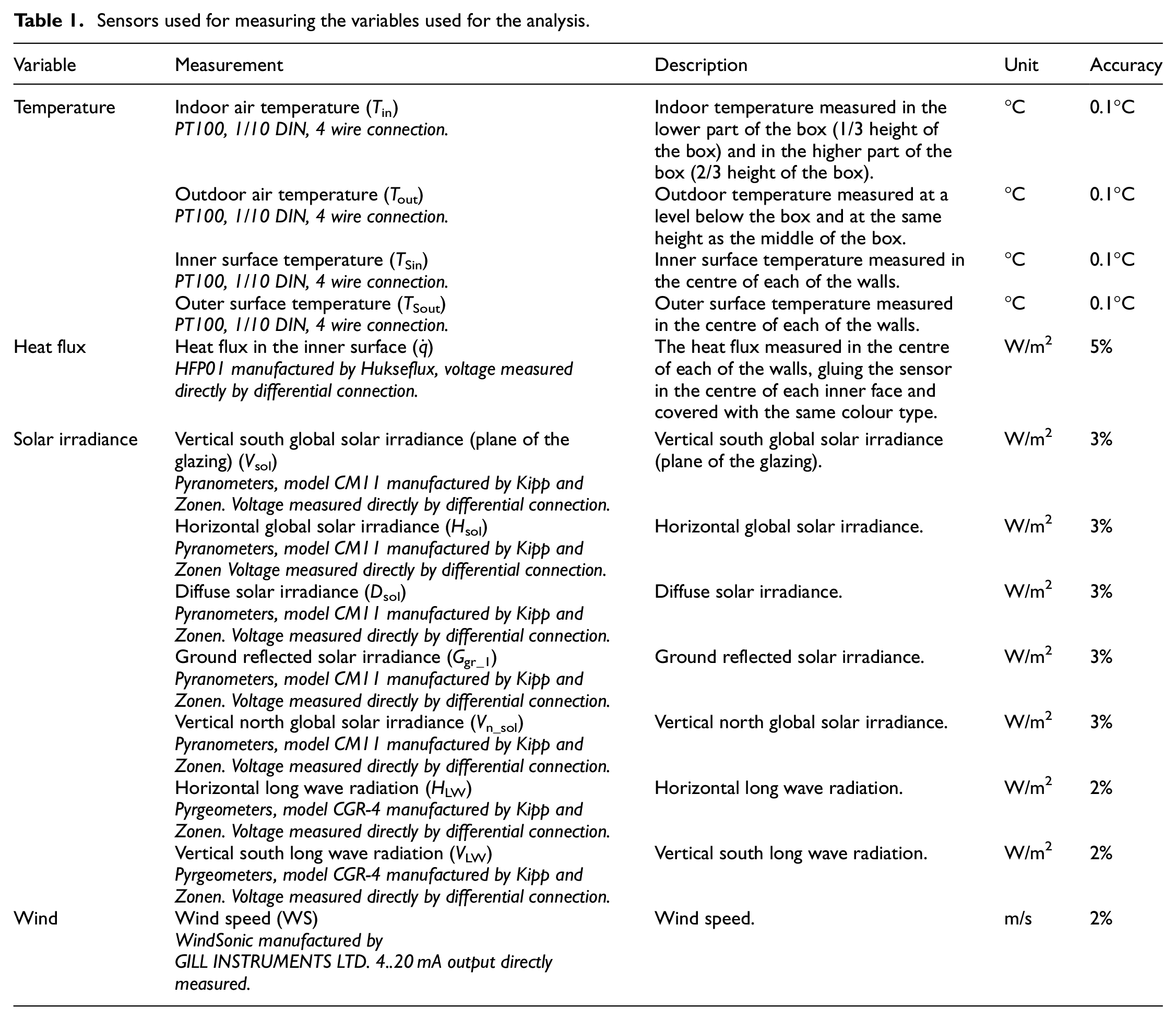
During the Round Robin Box tests, a wide range of variables were measured. In order to carry out a deeper analysis of the solar gains through the Round Robin Box’s different opaque faces (east, north and west walls, floor and ceiling), each of the faces was analysed individually. The Round Robin Box walls are named as follows: the glazing wall (the one with the window and orientated to the south), the east wall (the opaque wall orientated to the east), the west wall (the opaque wall orientated to the west), the north wall (the opaque wall orientated to the north), the ceiling wall (the opaque wall orientated to the sky) and the floor wall (the opaque wall orientated to the ground). The glazing wall was excluded from this study, analysing only the effect of the solar radiation in opaque walls. Among the measurements carried out during the Almeria Round Robin Box tests, Table 1 shows only the variables measured within the Round Robin Box experiment that are used during the proposed analysis in this research. It must be said that the resolution of the A/D converter is 16 bits. A full description of the experimental set up is included in the final report of Annex 58 (Jiménez, 2016).

Table 1.

Sensors used for measuring the variables used for the analysis.

Variable	Measurement	Description	Unit	Accuracy
Temperature	Indoor air temperature (Tin) PT100, 1/10 DIN, 4 wire connection.	Indoor temperature measured in the lower part of the box (1/3 height of the box) and in the higher part of the box (2/3 height of the box).	°C	0.1°C
	Outdoor air temperature (Tout) PT100, 1/10 DIN, 4 wire connection.	Outdoor temperature measured at a level below the box and at the same height as the middle of the box.	°C	0.1°C
	Inner surface temperature (TSin) PT100, 1/10 DIN, 4 wire connection.	Inner surface temperature measured in the centre of each of the walls.	°C	0.1°C
	Outer surface temperature (TSout) PT100, 1/10 DIN, 4 wire connection.	Outer surface temperature measured in the centre of each of the walls.	°C	0.1°C
Heat flux	Heat flux in the inner surface ( $\stackrel{·}{q}$ ) HFP01 manufactured by Hukseflux, voltage measured directly by differential connection.	The heat flux measured in the centre of each of the walls, gluing the sensor in the centre of each inner face and covered with the same colour type.	W/m2	5%
Solar irradiance	Vertical south global solar irradiance (plane of the glazing) (Vsol) Pyranometers, model CM11 manufactured by Kipp and Zonen. Voltage measured directly by differential connection.	Vertical south global solar irradiance (plane of the glazing).	W/m2	3%
	Horizontal global solar irradiance (Hsol) Pyranometers, model CM11 manufactured by Kipp and Zonen Voltage measured directly by differential connection.	Horizontal global solar irradiance.	W/m2	3%
	Diffuse solar irradiance (Dsol) Pyranometers, model CM11 manufactured by Kipp and Zonen. Voltage measured directly by differential connection.	Diffuse solar irradiance.	W/m2	3%
	Ground reflected solar irradiance (Ggr_1) Pyranometers, model CM11 manufactured by Kipp and Zonen. Voltage measured directly by differential connection.	Ground reflected solar irradiance.	W/m2	3%
	Vertical north global solar irradiance (Vn_sol) Pyranometers, model CM11 manufactured by Kipp and Zonen. Voltage measured directly by differential connection.	Vertical north global solar irradiance.	W/m2	3%
	Horizontal long wave radiation (HLW) Pyrgeometers, model CGR-4 manufactured by Kipp and Zonen. Voltage measured directly by differential connection.	Horizontal long wave radiation.	W/m2	2%
	Vertical south long wave radiation (VLW) Pyrgeometers, model CGR-4 manufactured by Kipp and Zonen. Voltage measured directly by differential connection.	Vertical south long wave radiation.	W/m2	2%
Wind	Wind speed (WS) WindSonic manufactured by GILL INSTRUMENTS LTD. 4..20 mA output directly measured.	Wind speed.	m/s	2%

Method

First of all, a detailed theoretical representation is provided on how solar radiation affects the inner surface heat flux of an opaque wall. This can be mathematically represented under steady-state assumptions, assuming that the dynamic effects are negligible in long-term analyses. This mathematical development aims to establish a relationship between the actual and the hypothetical heat flux on the inner surface in the absence of solar radiation; while also taking into account the usually known physical characteristics of typical opaque building envelope components. Finally, a relationship is established between these heat fluxes on the inner surface of the wall and the solar factor of opaque walls, for its theoretical estimation.

Once these equations have been theoretically represented, they are then incorporated into inverse dynamic modelling under different assumptions and approximations, and gradually increasing the detail of the physical representation together with the model complexity. Therefore, a wide range of candidate models has been proposed considering in detail the different physical phenomena occurring on the outermost surface of the wall. The physical parameters are estimated from these candidate models in order to compare them with the theoretical values and see which model’s values most closely approach reality. Moreover, the residuals of the models are analysed. Thus, the best model fits are found for all the opaque faces of the Round Robin Box for two different datasets, one in winter and one in summer, in order to be able to see the differences in the model performance and the corresponding results. Once the best fits have been found, the solar irradiance signal is removed in order to estimate the real weight it has on the inner surface heat flux through the estimation of the hypothetical inner surface heat flux. Finally, the g-values have also been estimated for each of the walls, using the difference between the real and hypothetical inner surface heat fluxes and these have been compared with the values obtained directly from the LORD software (Figure 3).

Figure 3.

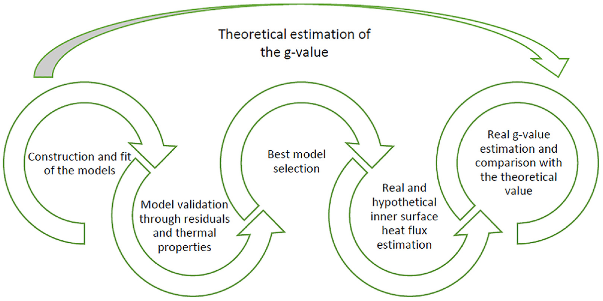
Methodology flowchart.

Detailed theoretical representation of how the solar radiation affects the inner surface heat flux of an opaque wall

Due to the heating effect of the solar radiation on the outer surface of opaque walls, the inner surface heat flux going outwards is reduced. This effect is mathematically quantified in this section for a general opaque wall under steady-state assumptions, presented in Figure 4 and later transmitted to the solar factor estimation. This mathematical development is also valid for any other opaque building envelope element facing solar radiation.

Figure 4.

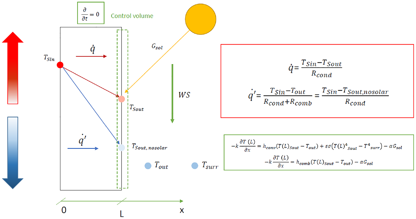
Energy balance representation in a massless control volume representing the outer surface of an opaque wall.

Even if the opaque elements of building envelopes are subjected to dynamic behaviour, doing a steady-state analysis can give very valuable results, since they operate for very long periods of time. For example, the ISO9869-1:2014 (ISO 9869-1, 2014) standard ‘Thermal insulation – Building elements – in situ measurement of thermal resistance and thermal transmittance’ describes the testing methodology to obtain, in-situ, the U-value of opaque walls using testing periods of at least 72 hours. During these tests, the change in the amount of heat stored in the element must be negligible when compared to the amount of heat going through the element. Of course, depending on the thermal mass and level of insulation of the element, the solar radiation effect on its outer surface will take more or less time to affect the inner surface heat flux; however, for a long period analysis, the dynamic effects become negligible and thus a steady-state analysis will be performed. Then, although this mathematical demonstration is presented using steady state conditions in order to simplify the demonstration, the modelling method presented afterwards considers the dynamic behaviour of the opaque faces using real, measured data.

In Figure 4, two inner surface heat fluxes are represented: the $\stackrel{·}{q}$ , which is the real inner surface heat flux considering the solar radiation effect; and ${\stackrel{·}{q}}^{\prime }$ , which is the hypothetical inner surface heat flux without considering the solar radiation effect. From the latter, it can be assumed that, due to the lack of the solar radiation effect in the T_Sout,nosolar used for its estimation, the ${\stackrel{·}{q}}^{\prime }$ will show higher values than $\stackrel{·}{q}$ . Then, to estimate the effect of the solar radiation on the inner surface heat flux, the aim of this mathematical development is to relate $\stackrel{·}{q}$ with ${\stackrel{·}{q}}^{\prime }$ , based on the typical physical knowledge on common opaque building envelope elements. Not surprisingly, since this section development assumes the steady-state assumption, the conduction heat flux will be the same in any other position within the opaque wall, including the outer surface. Then, applying the energy balance to the massless control volume representing the outer surface of the wall, we obtain equation (1).

$$\stackrel{·}{q}=-k\frac{\partial T(x=L)}{\partial x}=h_{\mathrm{conv}}(T_{\mathrm{Sout}}-T_{\mathrm{out}})+\epsilon \sigma ({T^4}_{\mathrm{Sout}}-{T^4}_{\mathrm{surr}})-\alpha G_{\mathrm{sol}}[\mathrm{W}/{\mathrm{m}}^2]$$

(1)

Equation (1) shows the three main terms related with three important phenomena that may affect the outer surface of the wall. The solar radiation is one. The effect of this phenomenon is considered in the last term of the formula ( $\alpha G_{\mathrm{sol}}),$ where α represents the outer surface solar absorptivity and G_sol represents the global solar irradiance incident on the outer surface of the wall.

The middle term, $\epsilon \sigma ({T^4}_{\mathrm{Sout}}-{T^4}_{\mathrm{surr}}),$ considers the heat exchange due to the long wave radiation on the outer surface of the wall. T_Sout is the real outer surface temperature of the wall, considering the solar radiation effect (see Figure 4). T_surr, as an effective temperature that simplifies the equation to the maximum extent by encompassing form factors within its non-measured nature, eliminating the need for their individual consideration. Furthermore, the parameters $\epsilon$ and $\sigma$ represent the emissivity of the walls’ outer surface and the Stefan Boltzmann constant (5.67 × 10⁻⁸ [W/m² K⁴]), respectively. However, the temperature of the surroundings (T_surr) will vary, depending on the wall. As shown in equation (1), for the vertical walls, T_surr must be used. Nevertheless, for the ceiling and the floor, T_sky and T_ground, respectively, must be used. In this research, the surrounding temperature and the sky temperature can be obtained thanks to the available measurements of the vertical south (V_LW) and the horizontal (H_LW) long wave radiation using equations (2) and (3), respectively.

$$T_{\mathrm{surr}}=\sqrt[4]{\frac{V_{\mathrm{LW}}}{\sigma }}\left[\mathrm{K}\right]$$

(2)

$$T_{\mathrm{sky}}=\sqrt[4]{\frac{H_{\mathrm{LW}}}{\sigma }}\left[\mathrm{K}\right]$$

(3)

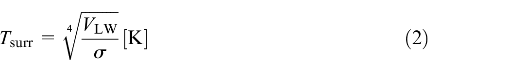
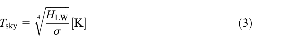
However, since no long wave radiation measurement is available for the ground temperature estimation, a good approximation of it is obtained, assuming the ground temperature tends to the sol-air temperature defined in ASHRAE (ASHRAE Handbook, 2005). So, equation (4) is taken from ASHRAE (ASHRAE Handbook, 2005) to estimate the ground temperature.

$$T_{\mathrm{ground}}=T_{\mathrm{out}}+\frac{\alpha \times G_{\mathrm{sol}}}{h_{\mathrm{comb}}}+\frac{\epsilon \times \Delta R}{h_{\mathrm{comb}}}\left[\mathrm{K}\right]$$

(4)

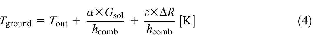
where T_out is the outdoor air temperature [K], $\alpha$ is the absorptance of the ground surface for the solar radiation [-], $G_{\mathrm{sol}}$ is the global solar irradiance incident on the ground surface [W/m²], h_comb is the combined coefficient of heat transfer by long wave radiation and convection at ground surface [W/m² K], $\epsilon$ is the hemispherical emittance of the ground surface [-] and $\Delta R$ is the difference between the long-wave radiation incident on the surface from the sky and surroundings and the radiation emitted by a blackbody at outdoor air temperature [W/m²]. Thus, equation (4) should provide very similar results to the real temperature of the ground surface.

However, the use of these temperatures considerably complicates this theoretical mathematical development. ASHRAE Handbook (2005) remarks that for vertical walls, in common practice, it can be assumed that T_surr ≈ T_out. In the case of the horizontal surfaces, it can be assumed that T_sky ≈ T_out−4°C. However, due to the difficulties in estimating the horizontal long wave radiation and, consequently, the sky temperature, this theoretical development assumes that T_sky ≈ T_out. The same assumption is made for the ground case (T_ground ≈ T_out). These assumptions are considered only for the development of this demonstration section, while the calculations carried out in the experimental section are done using the measured surrounding (equation (2)) and sky (equation (3)) temperatures and the estimated ground (equation (4)) temperature, instead of with the assumptions presented in this mathematical development.

Finally, the last term $(h_{\mathrm{conv}}(T_{\mathrm{Sout}}-T_{\mathrm{out}}))$ can be used to introduce the effect of the wind speed on the inner surface heat flux estimation. Therefore, a correlation between the wind speed and the convective heat transfer coefficient (h_conv) should be found and fixed. However, the convective heat transfer coefficient can also be estimated without considering the effect of the wind speed.

Once all the phenomena affecting the outer surface of the opaque wall have been theoretically presented, it is now possible to theoretically present the method used for quantifying the solar radiation effect on the inner surface heat flux of opaque walls.

The theoretical quantification of the solar radiation effect on the inner surface heat flux of opaque walls

Considering T_surr ≈ T_out and linearising the radiation heat exchange term of equation (1), as done in (Cengel, 2014), equation (5) and consequently equation (6), are obtained. Finally, combining the convective heat transfer coefficient (h_conv) with the linearised radiation heat transfer coefficient (h_rad), the combined convection-radiation heat transfer coefficient (h_comb = h_conv + h_rad) can be obtained, as represented in equation (7).

$$\stackrel{·}{q}=-k\frac{\partial T\left(L\right)}{\partial x}=h_{\mathrm{conv}}(T_{\mathrm{Sout}}-T_{\mathrm{out}})+\epsilon \sigma ({T^4}_{\mathrm{Sout}}-{T^4}_{\mathrm{out}})-\alpha G_{\mathrm{sol}}[\mathrm{W}/{\mathrm{m}}^2]$$

(5)

$$\stackrel{·}{q}=-k\frac{\partial T\left(L\right)}{\partial x}=h_{\mathrm{conv}}(T_{\mathrm{Sout}}-T_{\mathrm{out}})+h_{\mathrm{rad}}(T_{\mathrm{Sout}}-T_{\mathrm{out}})-\alpha G_{\mathrm{sol}}[\mathrm{W}/{\mathrm{m}}^2]$$

(6)

$$\stackrel{·}{q}=-k\frac{\partial T\left(L\right)}{\partial x}=h_{\mathrm{comb}}(T_{\mathrm{Sout}}-T_{\mathrm{out}})-\alpha G_{\mathrm{sol}}[\mathrm{W}/{\mathrm{m}}^2]$$

(7)

Since we assume the steady-state conditions, $\stackrel{·}{q}$ can also be calculated from the inner surface temperature to the outer surface temperature by means of equation (8). R_cond represents the sum of all the conduction resistances of the opaque wall, represented in Figure 4. Note that the analysis could also be performed from the indoor air temperature by also considering the inner surface convection-radiation heat transfer coefficient added to the R_cond. As in the models developed below; in order to avoid uncertainties associated with the inner surface convection-radiation heat transfer coefficient, the equations consider the inner surface as their boundary. Then, this mathematical development has been performed from the inner surface instead of from the indoor air.

$$\stackrel{·}{q}=-k\frac{\partial T\left(L\right)}{\partial x}=\left(\frac{T_{\mathrm{Sin}}-T_{\mathrm{Sout}}}{R_{\mathrm{cond}}}\right)[\mathrm{W}/{\mathrm{m}}^2]$$

(8)

Combining equations (7) and (8), we can solve for T_Sout as done in equation (9).

$$\begin{array}{l}\left(\frac{T_{\mathrm{Sin}}-T_{\mathrm{Sout}}}{R_{\mathrm{cond}}}\right)=\frac{1}{R_{\mathrm{comb}}}(T_{\mathrm{Sout}}-T_{\mathrm{out}})-\alpha G_{\mathrm{sol}}\\ T_{\mathrm{Sout}}=\frac{T_{\mathrm{Sin}}{R}_{\mathrm{comb}}+T_{\mathrm{out}}{R}_{\mathrm{cond}}+\alpha G_{s\mathrm{ol}}{R}_{\mathrm{cond}}{R}_{\mathrm{comb}}}{R_{\mathrm{cond}}+R_{\mathrm{comb}}}\left[°\mathrm{C}\right]\end{array}$$

(9)

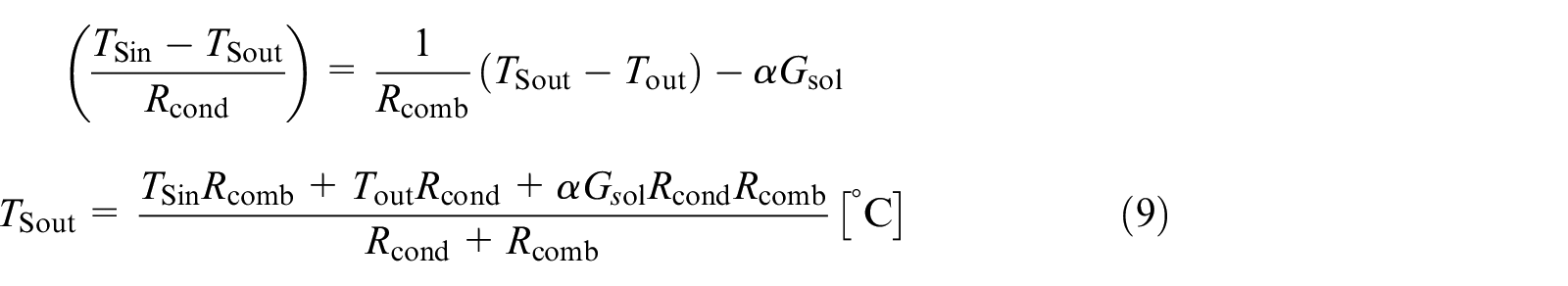
With equation (9), a mathematical expression of the real outer surface temperature has been obtained, based on the inner surface temperature, the outdoor air temperature, the global solar irradiance incident on the outermost surface of the opaque wall and the typical physical parameters known for a general opaque wall. Now, the real inner surface heat flux $\stackrel{·}{q},$ which considers the solar radiation incident on the outermost surface of the wall, and the hypothetical inner surface heat flux ${\stackrel{·}{q}}^{\prime },$ that would occur in the absence of solar radiation on the outermost surface of the opaque wall, are both related. The form the hypothetical inner surface heat flux $\stackrel{·}{q}\prime$ would have in the absence of solar radiation is shown in equation (10).

$$\stackrel{·}{q}\prime =\left(\frac{T_{\mathrm{Sin}}-T_{\mathrm{out}}}{R_{\mathrm{cond}}+R_{\mathrm{comb}}}\right)[\mathrm{W}/{\mathrm{m}}^2]$$

(10)

If the T_Sout expression of equation (9) is introduced in the expression of equation (8), the right-hand term of equation (10) must be searched for in the development. Once this term has been identified, we can conclude that the remaining terms, excluding the right-hand term of equation (10), represent the influence of solar radiation on the heat flux of the inner surface of the wall under analysis.

$$\begin{array}{l}\stackrel{·}{q}=\frac{T_{\mathrm{Sin}}-\left(\frac{T_{\mathrm{Sin}}{R}_{\mathrm{comb}}+T_{\mathrm{out}}{R}_{\mathrm{cond}}+\mathrm{\alpha }{G}_{\mathrm{sol}}{R}_{\mathrm{cond}}{R}_{\mathrm{comb}}}{R_{\mathrm{cond}}+R_{\mathrm{comb}}}\right)}{R_{\mathrm{cond}}}[\mathrm{W}/{\mathrm{m}}^2]\\ \stackrel{·}{q}=\frac{T_{\mathrm{Sin}}-T_{\mathrm{out}}}{(R_{\mathrm{cond}}+R_{\mathrm{comb}})}-\frac{\mathrm{\alpha }{G}_{\mathrm{sol}}{R}_{\mathrm{comb}}}{(R_{\mathrm{cond}}+R_{\mathrm{comb}})}=\stackrel{·}{q}\prime -\frac{\mathrm{\alpha }{G}_{\mathrm{sol}}{R}_{\mathrm{comb}}}{(R_{\mathrm{cond}}+R_{\mathrm{comb}})}[\mathrm{W}/{\mathrm{m}}^2]\end{array}$$

(10)

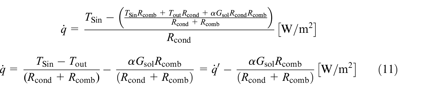
Analysing equation (11), it is found that the real heat flux on the inner surface of the wall $\stackrel{·}{q}$ is equal to the hypothetical inner surface heat flux ${\stackrel{·}{q}}^{\prime },$ as if no solar radiation effect were considered, minus the term $\frac{\mathrm{\alpha }{G}_{\mathrm{sol}}{R}_{\mathrm{comb}}}{(R_{\mathrm{cond}}+R_{\mathrm{comb}})},$ which represents the reduction effect of the solar radiation on the inner surface heat flux. Thus, the theoretical quantification of the effect of the solar radiation on the inner surface heat flux of opaque walls under steady-state conditions can be obtained by means of equation (12).

$${\stackrel{·}{q}}_{\mathrm{dif}}=\stackrel{·}{q}\prime -\stackrel{·}{q}=\frac{\mathrm{\alpha }{G}_{\mathrm{sol}}{R}_{\mathrm{comb}}}{(R_{\mathrm{cond}}+R_{\mathrm{comb}})}[\mathrm{W}/{\mathrm{m}}^2]$$

(12)

If this term is large enough, it can make the inner surface heat flux negative; remember that a negative inner surface heat flux is actually a heat gain to the interior of the building. Moreover, for long enough periods, where the heat accumulation term within the wall becomes negligible in comparison with the rest of heat exchanges within the wall (Chávez et al., 2019), it is also possible to check the period averaged effect the solar radiation has on the inner surface heat flux of opaque building elements by using the period averaged form of equation (12) presented in equation (13).

$$\overline{\stackrel{·}{q}\prime }-\overline{\stackrel{·}{q}}=\frac{\mathrm{\alpha }\overline{G_{\mathrm{sol}}}{R}_{\mathrm{comb}}}{(R_{\mathrm{cond}}+R_{\mathrm{comb}})}[\mathrm{W}/{\mathrm{m}}^2]$$

(13)

Estimating the ${\stackrel{·}{q}}_{\mathrm{dif}}$ using this formula proves to be challenging due to the lack of accurate knowledge regarding the physical parameters of the wall or ceiling (α and $R_{\mathrm{comb}}$ ). While it is mathematically representable with this formula, the experimental section outlines an alternative procedure that uses real, measured data to estimate this difference. Once the theoretical quantification of the solar radiation’s effect on the inner surface heat flux of opaque walls has been established, it becomes feasible to establish a relationship with the estimation of the solar factor.

The theoretical quantification of the solar factor of opaque walls

Making a parallelism with the solar factor (g-value) concept for windows, the solar factor of an opaque wall under steady-state conditions could be defined using the following expression:

$$g-\mathrm{valu}{\mathrm{e}}_{\mathrm{wall}}=\frac{\stackrel{·}{q}\prime -\stackrel{·}{q}}{G_{\mathrm{sol}}}[-]$$

(14)

where equation (14) represents the proportion of the total incident solar radiation that enters through the opaque wall. Of course, another way of obtaining the solar factor of the opaque walls could be obtained by introducing equation (12) in equation (14), as shown in equation (15).

$$g-\mathrm{valu}{\mathrm{e}}_{\mathrm{wall}}=\frac{\frac{\mathrm{\alpha }{G}_{\mathrm{sol}}{R}_{\mathrm{comb}}}{(R_{\mathrm{cond}}+R_{\mathrm{comb}})}}{G_{\mathrm{sol}}}=\frac{\alpha R_{\mathrm{comb}}}{(R_{\mathrm{cond}}+R_{\mathrm{comb}})}[-]$$

(15)

It is important to present both equations (14) and (15), since equation (14) permits us to estimate the solar factor of an opaque element based on in-situ measurements; while equation (15) only allows us to estimate the solar factor based on the physical parameters of the wall or ceiling. The use of equation (15) has a problem; although R_cond can be obtained with a high accuracy, based on the typical construction material properties; the solar absorptivity ( $\alpha$ ) values of the outermost surfaces of the building components are not always known with a high accuracy and, in real life, the combined convection-radiation thermal resistance (R_comb) is time dependent. Many standards fix this R_comb at 0.04 m² K/W (ISO 6946:2017, 2017).

Nevertheless, equation (14) would permit us to obtain the solar factor of the opaque element based on in-situ measurements of the inner surface heat flux ( $\stackrel{·}{q}$ ), the estimation of the hypothetical inner surface heat flux ( $\stackrel{·}{q}\prime$ ) in the absence of solar radiation and the incident global solar irradiance measurement on the outer surface of the opaque element. However, the use of equation (14) has two problems; the first is the impossibility of measuring the hypothetical inner surface heat flux ( $\stackrel{·}{q}\prime$ ), since it is not real. This problem can be overcome by fitting a model of the opaque building envelope using measured data and system identification techniques. Once the model parameters have been identified, they can be fixed and the inner surface heat flux estimated by running the fitted model without including the signal of the solar irradiance on the outermost surface of the opaque element. Thus, the hypothetical inner surface heat flux ( $\stackrel{·}{q}\prime$ ) would be obtained. The procedure for obtaining this parameter is detailed in the experimental section.

The second problem is the lack of steady-state conditions for in-situ opaque elements in real life. The latter can be overcome by using sufficiently long period averaged values for $\stackrel{·}{q}$ , $\stackrel{·}{q}\prime$ and $G_{\mathrm{sol}}$ . That is, instead of using equation (14) with instantaneous values, periods of several days must be analysed and the period averaged $\overline{\stackrel{·}{q}}$ , $\overline{\stackrel{·}{q}\prime }$ and $\overline{G_{\mathrm{sol}}}$ values should be used, as in equation (16). An example of these three variables that must be period averaged can be seen in Figure C1 ( $\overline{\stackrel{·}{q}}$ and $\overline{\stackrel{·}{q}\prime }$ ) and Figure A8 ( $\overline{G_{\mathrm{sol}}}$ ).

$$g-\mathrm{valu}{\mathrm{e}}_{\mathrm{wall}}=\frac{\overline{\stackrel{·}{q}\prime }-\overline{\stackrel{·}{q}}}{\overline{G_{\mathrm{sol}}}}[-]$$

(16)

Due to the difficulties of accurately estimating the solar factor using equation (15), equation (16) is used later in this work. Thus, the problems related with accurately unknown parameters can be avoided, since it is possible to estimate the g-value_wall through the estimation of the hypothetical inner surface heat flux using real measured data. Thus, the validity of equations (13) and (16), by means of a real case using inverse dynamic modelling, can be proved on a practical basis. This real case is the previously presented Round Robin Box test. Even if many global solar irradiance measurements are available for different orientations of the Round Robin Box test, the east and west walls did not have measurements for the global solar irradiance on them. The beam radiation ratio method (Duffie and Beckman, 2013) has been used to estimate the missing solar irradiance values. Once this has been done, the following section can present the experimental validation using inverse dynamic modelling.

Detailed experimental representation of how the solar radiation affects the inner surface heat flux of an opaque wall

Fit and validation of the models of the opaque elements of the Round Robin Box

Once all the global solar irradiance data have been made available for the Round Robin Box walls, ceiling and floor, the corresponding solar factor of each of these elements is estimated using the LORD software (Gutschker, 2003; Gutschker, 2008). LORD is a software package used for parameter identification in mathematical models. It estimates optimal values for unknown parameters based on measured or simulated data. The software employs advanced optimisation algorithms to minimise the difference between observed and predicted data. Parameter identification with LORD aids in experimental design, model calibration, property estimation and process optimisation. Users can optimise and simplify their models by analysing the statistical output, such as Principal Component Analysis. Since LORD is an estimation software based on parameter identification of RC models, it is able to estimate the U-value and the g-value of the wall, drawing on the provided input data. Before developing the proposed method, the provided data have been analysed to identify whether there are missing values or irregularities. Once the measurements have been checked and all the variables have been identified, the data to be used are selected. In this case, the variables selected to construct the analysed models are the inner surface temperature (T_Sin), the inner surface heat flux ( $\stackrel{·}{q}$ ), the outer surface temperature (T_Sout), the outdoor air temperature (T_out), the wind speed (WS), the surrounding, sky or ground temperature (T_surr, T_sky or T_ground) and the corresponding global solar irradiance (G_sol) on each surface. Each model will combine them differently, as shown in the following section. However, the inner surface heat flux has been chosen as the output variable in the eight different models created. All these measured input variables of the models are shown in Appendix A.

Construction and fit of candidate models for walls, ceiling and floor

Once all the data have been checked and divided into smaller periods, the different models can be considered and fitted using the LORD software by estimating the models’ parameters through measured, experimental data. This software offers the possibility of setting minimum and maximum limit values for the parameters that need to be identified. Thus, the parameter fitting can be done more efficiently within a reasonable, realistic range for each parameter. Of course, following identification, a check has always been done to make sure that the obtained fitting parameters do not lie close to the imposed limits. The models consider every phenomenon mentioned in the theoretical section; so, through these models, it is possible to identify accurately the dynamic behaviour of each opaque face using real, measured data.

The first case to be fitted is the simplest, the surface to surface case (Model 1, M1), shown in Figure 5(a). The only variables introduced in this model are the temperatures at both surfaces (inner and outer) and the inner surface heat flux. The first node represents the inner node, including the inner surface temperature and the inner surface heat flux. The A₁ value represents the aperture of the heat flux in this node, which corresponds to one for all the models in this case, since the total heat flux on the inner surface of the wall is actually measured and it is known that 100% of it crosses the wall’s inner surface. However, node five represents the outermost surface and is linked to the outer surface temperature. In conclusion, this model represents the wall, without considering any phenomena occurring in the internal or external environments.

Figure 5.

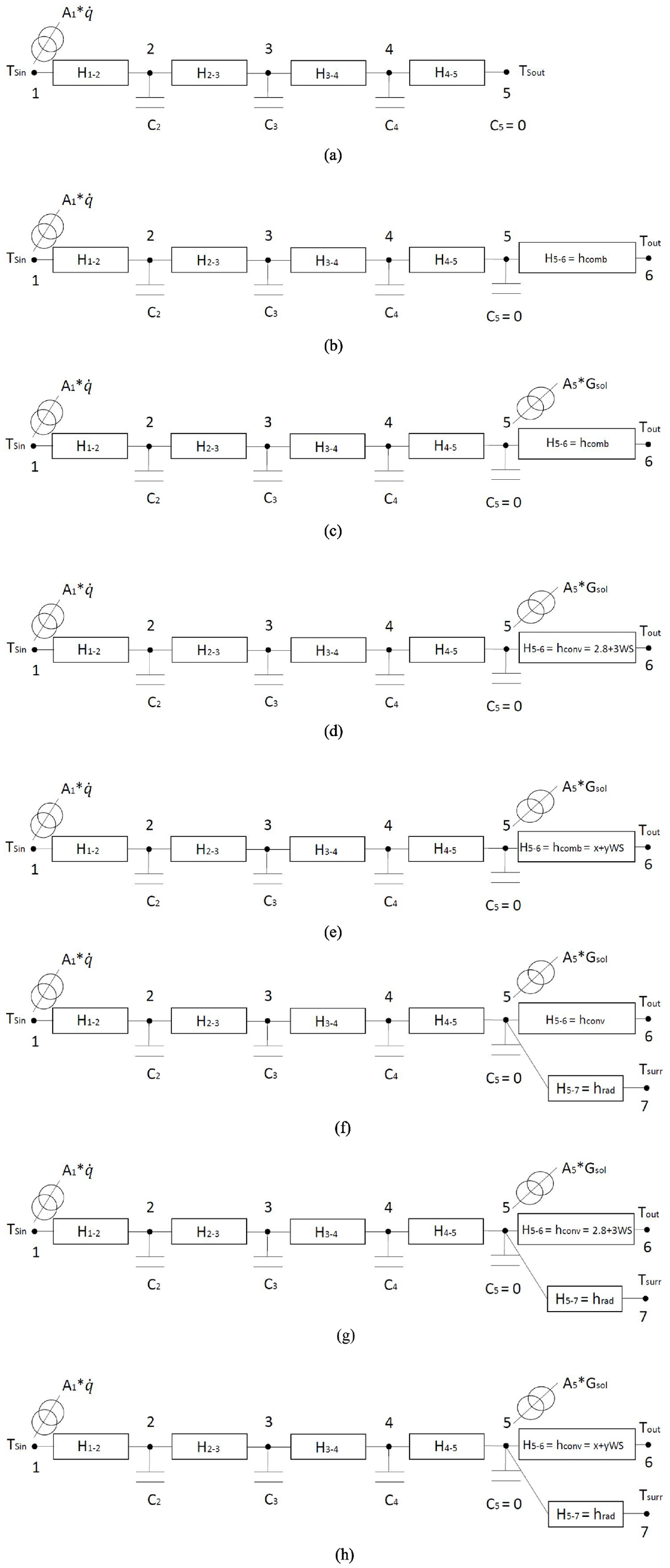
All the candidate models: (a) Model 1, (b) Model 2, (c) Model 3, (d) Model 4, (e) Model 5, (f) Model 6, (g) Model 7 and (h) Model 8.

As justified in the theoretical section, the outermost surface node is assumed to be a massless node where the energy balance is carried out on the outer surface. Thus, it is considered that the thermal capacitance at this node is equal to 0 (C₅ = 0). Following the logic for discretising walls into RC models, the closest thermal resistance (R_4–5) to this node must also be very small. In other words, the higher the thermal resistance R_4–5 value is, the wider the layer of wall considered by this thermal resistance should be. Then, the wider the R_4–5 is, the higher the capacity C₅ this layer should have associated. Therefore, in order to keep R_4–5 low enough to carry out the proposed energy balance in node 5, this value has been limited to 1% or lower than the total theoretical thermal resistance of the wall (R_w), where the surface to surface R_w = 1.93 m² K/W. Therefore, the thermal resistance R_4–5 should not exceed the value of 0.0193 m² K/W. The LORD software estimates the thermal conductance (this is the inverse of the thermal resistance (R_W = 1/H_W)), which means that the thermal conductance should be high for H_4–5. Then, this parameter will be limited, fixing 51.8 W/m² K as the lowest limit. For the rest of the model conductances, a wide range has been imposed for their identification.

Once the surface to surface model provides reliable parameters (thermal capacitance and conductance) and a proper fit of the inner surface heat flux, it is possible to start working with new models, including the external phenomena affecting the outermost surface. The reliability of the models is ensured according to two criteria. First, the residual analysis assessing the model fit and selecting the models with the lowest RMSE values for the residuals. Additionally, checking that the deviations of the estimated thermal resistances are not too far from the theoretical values (lower than a 10% of deviation). It is therefore necessary to include an extra node in the model, as shown in Figure 5(b), to include the external effects. This model (Model 2, M2) represents the case without considering any of the outer environmental phenomena in detail. In other words, the convection and the long wave radiation effects are considered through a constant conductance, while the signal including the solar irradiance data is not considered at all.

This Model 2 has six nodes. The first is maintained as in the surface to surface model. However, the link to the outer surface temperature is removed from node five and the outdoor air temperature is included in node six. The thermal conductance and capacitances obtained in the surface to surface model are fixed between nodes one and five, since they should not vary, depending on the influence of the external environment and they already represent a proper approximation of the theoretical thermal properties of the wall. Then, the only new parameter to be estimated is H_5–6, the external surface combined heat transfer coefficient (named h_comb in the theoretical section). This parameter has also been estimated based on the ISO 6946 (ISO 6946:2017, 2017), where a theoretical value has been obtained for this parameter for verification.

The third model tested is the one considering the influence of the solar radiation on the outer surface (Model 3, M3). The only difference between this Model 3 in Figure 5(c), compared with the previous Model 2 in Figure 5(b), is the incorporation of the global solar irradiance (G_sol) in node five. Together with this variable, the software also includes an extra parameter named A₅. This parameter represents the solar absorptivity of the outer surface wall, which also needs to be estimated. Then, the only two parameters that need to be estimated in this Model 3 are the previously mentioned H_5–6 combined conductance and the solar absorptivity (A₅). This solar absorptivity has been limited to between 0 and 1, always checking after identification that the estimate has not gone to one of the limits.

The next phenomenon analysed in detail is the wind speed. Therefore, the same model structure as in Figure 5(c) is taken. However, in this case, instead of using a single conductance for the estimation of H_5–6 (or h_comb), a wind dependent function implemented through LORD software is used. The wind speed analysis is performed in two different manners; as in Model 4 (M4, see Figure 5(d)), where H_5–6 is estimated using a specific correlation function representing solely the convective coefficient dependant on wind speed (h_conv) (see equation (17), taken from Watmuff et al., 1977); or as in Model 5 (M5, see Figure 5(e)), where H_5–6 is estimated using an identifiable correlation function ( $h_{\mathrm{comb}}=x+y\times \mathrm{WS}$ ). Here, during the model fit, within the identifiable x and y parameters, the long wave radiation and convective effects (h_comb) can be considered.

$$h_{\mathrm{conv}}=2.8+3\times \mathrm{WS}[\mathrm{W}/{\mathrm{m}}^2\mathrm{K}]$$

(17)

Thus, in the case of M4, since a pure convective coefficient is used, and there is no identifiable parameter for the H_5–6 estimation, only the heat transfer due to convection (h_conv) has been considered in H_5–6, excluding the heat transfer due to long wave radiation. However, in M5, part of the long wave radiation effect is considered within the x and y parameters during their identification. During the analysis, both cases (M4 and M5) have been tested and compared. Then, since for M4 only the solar absorptivity (A₅) is estimated, it is possible for the model to estimate the effect of the long wave radiation within this parameter. However, as commented before, since in M5, apart from the solar absorptivity (A₅), the parameters of the correlation function are also estimated, the long wave radiation effect can be reflected in these x and y parameters.

The next tested model (Model 6, M6) also considers the effect of the long wave radiation together with the solar radiation and the convection. So a new branch has been included in Model 3 in Figure 5(c), as shown in Model 6 in Figure 5(f), where there is an extra branch between the nodes 5 and 7 in the model. The surrounding temperature is included in node 7, which has been estimated using equation (2). Therefore, the parameters estimated by the software when identifying this model are: the convective thermal conductance (instead of the combined thermal conductance of Figure 5(c)) between nodes 5 and 6 (H_5–6), the linearised long wave radiation thermal conductance between nodes 5 and 7 (H_5–7) and the solar absorptivity (A₅). The conductance H_5–7 corresponds to the previously presented radiation heat transfer coefficient h_rad. This h_rad could be estimated using the following equation (18):

$$h_{\mathrm{rad}}=\epsilon \sigma ({T_{\mathrm{Sout}}}^2+{T_{\mathrm{surr}}}^2)(T_{\mathrm{Sout}}+T_{\mathrm{surr}})[\mathrm{W}/{\mathrm{m}}^2\mathrm{K}]$$

(18)

The emissivity ( $\epsilon$ ) of the wall must also be fixed between 0 and 1. Therefore, the lowest h_rad value that can be obtained would be 0. However, the highest value would depend on the measured variables. In this case, $\epsilon$ would be one. Since the Stefan Boltzmann value ( $\sigma$ ) is constant, the maximum h_rad would depend on the surface and the surrounding temperature. In order to estimate this maximum possible value, the h_rad value of each hourly data from the total selected dataset is estimated. Thus, the highest limit of this H_5–7 will be different for each of the walls, since it depends on their surface and surrounding temperature. In the case of the ceiling and the floor, the same procedure is followed, but instead of using the T_surr, the corresponding temperature (T_sky or T_ground) is used. Then, in this procedure, unlike in the theoretical development, where the temperatures were simplified for calculation, the real, measured temperatures are used for each of the walls.

Once the previous models have considered modelling for all the outer environmental phenomena, two new models (Model 7, M7 and Model 8, M8) are proposed and analysed, taking into account all the detailed phenomena together. The structure of the model used for this case is the same as that used in Model 6 in Figure 5(f). However, the effect of the wind speed is introduced within the convective coefficient, using the fixed correlation (M7) of equation (17) or leaving the parameters of the correlation freely identifiable (M8). Both cases are analysed again, but in this case, together with the solar radiation and the long wave radiation affecting the outer surface of the corresponding wall, as shown in Figures 5(g) for Model 7 (M7) and 5(h) for Model 8 (M8).

It must be said that, in the development of the theoretical section, the h_conv and the h_rad have been considered together as h_comb in order to simplify the calculation. However, as shown in this section, when implementing the models, each heat transfer coefficient has been considered and estimated individually against their respective real, measured temperatures.

Finally, since in this case some of the theoretical values are known, all the estimated parameters in each of the models are compared with their respective theoretical values, as explained in the next section, and the best fits are selected by comparing the estimated and measured inner surface heat flux values. The best-fit selection is carried out using the Root Mean Square Error (RMSE). Thus, it is possible to estimate the model that best represents the reality of the walls’ outermost surface and it is used for the inner surface heat flux analysis. This procedure has been repeated for two periods (one in winter and one in summer).

Physical validation criteria applied to the fitted models

As discussed in the previous section, in order to develop a proper validation of the obtained model results based on measured data, the theoretical thermal and geometrical properties of the box have been used. Thus, it is possible to estimate the design transmittance (U-value) of the walls, floor and ceiling. The information concerning the walls, floor and ceiling is detailed in Jiménez (2016). So the theoretical U-value is estimated using the following formula:

$$U=\frac{1}{R_{\mathrm{si}}+R_{\mathrm{W}}+R_{\mathrm{comb}}}[\mathrm{W}/{\mathrm{m}}^2\mathrm{K}]$$

(19)

where R_W =  $\sum _{i=1}^N(l_i/k_i)$  = (l₁/k₁) + (l₂/k₂)+(l₃/k₃)+…+(l_N/k_N) [m² K/W] and l_i and k_i are the thickness and thermal conductivity of the layers that form the wall. The variable i is the sum index to which an initial value of 1 is given as the lowest limit and this makes up the range of all the integer values until the upper limit N is reached. This N value will vary depending on the layer quantity forming the wall. However, R_si and R_comb are, respectively, the inner and outer surface thermal resistances of the wall. The R_si and R_comb (R_conv and R_rad in parallel) values are standard constant values taken from (ISO 6946:2017, 2017). The obtained theoretical U-value from equation (19) is 0.48 W/m²K. The fact that, in the tested basic model M1 considered in the previous section, the internal first node is considered to be the inner surface instead of the indoor air, must be taken into account. Then, the estimated value from equation (19) is an air to air value, while the value obtained from M1 is a surface to surface or a surface to air value for the models M2 to M8 presented hereafter. The walls’ theoretical thermal resistance surface to surface can be calculated as in equation (20), since the thicknesses and the thermal conductivities of all the walls’ materials are known.

$$R_{\mathrm{W}}=\sum \frac{l_i}{k_i}[{\mathrm{m}}^2\mathrm{K}/\mathrm{W}]$$

(20)

The estimated theoretical R_w result is 1.93 m² K/W (equation (20)). This value should be compared with the total thermal resistance value obtained from Model 1 (M1). However, since LORD provides the value of each of the thermal conductances of the fitted model, it is possible to calculate the thermal resistance (R_W) of the wall (since R_W = 1/H_W = (1/H_1–2) + (1/H_2–3) + (1/H_3–4)+…+(1/H_N−1−N) [m² K/W]), again using the sum of each of the layers’ thermal resistance from i = 1–2 to i = N − 1 – N and comparing the results of this thermal resistance with the one obtained from the design values.

Moreover, it is also possible to theoretically estimate the total thermal resistance of the best model found from those proposed in the previous section, since the outer surface thermal resistance of the wall is also known, as discussed previously. Therefore, equation (21) is used.

$$R_T=\sum \frac{l_i}{k_i}+R_{\mathrm{comb}}[{\mathrm{m}}^2\mathrm{K}/\mathrm{W}]$$

(21)

Thus, the theoretical R_T value for this case would be 1.97 m² K/W, since the R_comb value is taken from (ISO6946:2007) and its value is 0.04 m² K/W. Then, the best estimated model, from all the models presented in the previous section, should be able to estimate a similar R_T result to the theoretical R_T value. However, since R_comb is a standard value, the estimations of LORD could differ from the theoretical values.

Finally, it must be said that the rest of the physical parameters, such as the solar absorptivity, have also been useful in the validation process of the models. Although this value is unknown, a theoretical solar absorptivity value of 0.6 could be assigned for the fibre cement material (Cengel, 2014). Nevertheless, due to the fact that the fibre cement is coated with white paint, its solar absorptivity value may approximate 0.2 (Chávez et al., 2019). Consequently, in order to mitigate the highest level of uncertainty in the calculation and results, a range of solar absorptivity between 0.2 and 0.6 will be considered for the purpose of comparison and value estimation throughout this study.

Obtaining the hypothetical inner surface heat flux without considering the solar radiation effect

The estimation of the hypothetical inner surface heat flux is carried out based on the previous model fits and the proper validation of the models. Following a deep analysis of the models presented, one is selected as the best at representing the reality for each of the walls. As shown in the results and discussion section, Models 7 and 8 are the best for almost every wall. Then, these two models are used for the estimation of the solar radiation effect on the inner surface heat flux.

Figure 6(a) and (b) show the same number of nodes, respectively, as the M7 and M8. Moreover, the same H_i and C_i values estimated during the fitting of these models are used for each of them. The rest of the parameters are also fixed during the simulation. The only difference between the models M9 and M10, as compared to the models M7 and M8, is the absence of the solar irradiance signal on node 5. If solar irradiance is not provided for the model, it will simulate the hypothetical inner surface heat flux ( $\overline{\stackrel{·}{q}\prime }$ ) for the wall when subjected to the same inner surface temperature, the same outdoor air temperature, the same surrounding/sky/ground temperature and the same wind speed, but without the incident solar radiation striking the outermost surface of the wall.

Figure 6.

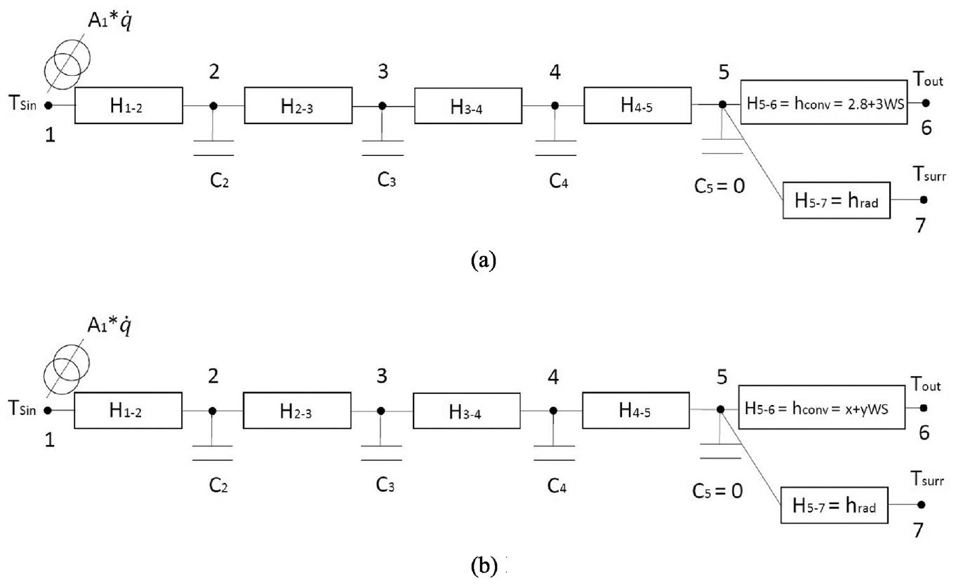
Best identified models modified for inner surface heat flux estimation without the solar radiation effect: (a) Model 9 and (b) Model (10).

Finally, once the inner surface heat fluxes, the inner surface heat flux considering the solar radiation effect ( $\stackrel{·}{q}$ ) and the hypothetical inner surface heat flux without considering the solar radiation effect ( ${\stackrel{·}{q}}^{\prime }$ ) have all been estimated, it is possible to estimate the effect of the solar radiation on the inner surface heat flux using equation (13). Moreover, the effect of the solar radiation has also been quantified as a percentage using equation (22) for the analysed periods.

$${\stackrel{.}{q}}_{\%}=\frac{\overline{{\stackrel{.}{q}}^{\prime }}-\overline{\stackrel{.}{q}}}{\overline{\stackrel{.}{q}}}\times 100[\%]$$

(22)

Solar factor (g-value_wall) estimation

The estimation of the wall g-value has been performed in two different manners; first using LORD, which automatically provides the g-value_wall when fitting the model. Then, the value estimated by LORD is compared with the g-value_wall estimated using equation (16) for each wall. The theoretical g-value_wall considering the constructive data is also calculated by means of equation (15) as follows:

$$\begin{array}{l}g-\mathrm{valu}{\mathrm{e}}_{\mathrm{wall}\_\min }=\frac{\alpha R_{\mathrm{comb}}}{(R_{\mathrm{cond}}+R_{\mathrm{comb}})}=\frac{0.2x0.04}{(1.93+0.04)}=0.004[-]\\ g-\mathrm{valu}{\mathrm{e}}_{\mathrm{wall}\_\max }=\frac{\alpha R_{\mathrm{comb}}}{(R_{\mathrm{cond}}+R_{\mathrm{comb}})}=\frac{0.6x0.04}{(1.93+0.04)}=0.012[-]\end{array}$$

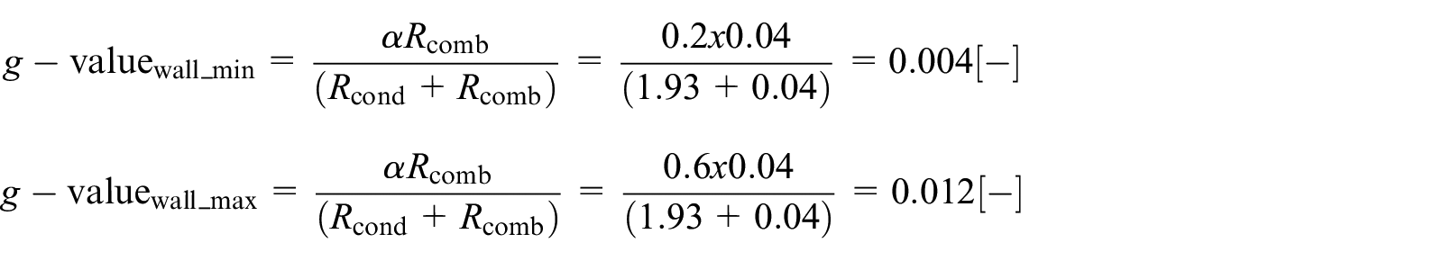
In this case, due to the utilisation of a theoretical solar absorptivity range, as previously mentioned, a maximum and a minimum theoretical g-value will be obtained. Subsequently, in the results and discussion section, it will be necessary to verify that all values obtained lie within this specified range.

Results and discussion

In order to perform this analysis, one sunny summer period and one cloudy winter period have been analysed. Period 1 (summer period) starts 18th June and ends 26th June 2013; while period 2 (winter period) starts 19th December and ends 21st December 2013. Obviously, the summer period shows higher solar irradiance values than the winter period. Moreover, for the winter case, the period with the consistently lowest solar irradiance has been consciously selected in order to study two extreme periods.

Validity analysis of the models

As explained above, in order to select the best model, it has been necessary to carry out an exhaustive analysis and validation of the residuals of the models and the identified U-value, together with the rest of the physical parameters (such as the solar absorptivity), estimated for each of the walls. Therefore, the first step of the model selection has been the analysis of the residuals through the RMSE. All the RMSE values obtained for each of the models are presented in Figure 7. All these values have been analysed one by one in order to find the lowest residual results.

Figure 7.

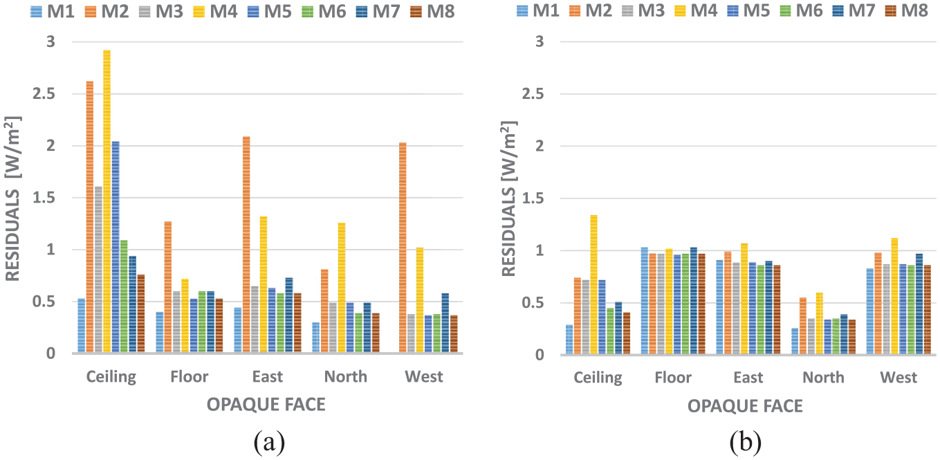
The RMSE residual values for the corresponding model and opaque face for the selected periods in [W/m²]: (a) Period 1 (summer) and (b) Period 2 (winter).

As can be seen in Figure 7, from all the models, M1 generally shows the lowest residual and, accordingly, the best results in terms of residual levels. However, since it is not possible to use this to estimate the effect the solar radiation has on the inner surface heat flux, it is only used as a reference to fit the rest of the models. For the other models, despite the difference in the obtained residual values being low in general, the lowest residuals were obtained for M8. However, for some of the walls, the same value as that obtained for Model 8 was also obtained for Model 5 or Model 6. Nevertheless, Model 8 is preferred over Models 5 and 6 because its residuals are at the lowest level for all the wall orientations, under both high and low levels of solar radiation and in this sense they have a wider generality. Additionally, since Model 8 represents the closest convective and radiative effects to reality occurring on the external surface of the wall, as they are estimated through the monitored real data, it is considered to be the best approach for this research. In other words, Model 8 is the one that considers the highest number of physical effects occurring in reality, so it is considered to be the best.

In order to justify the fact that Model 8 provides the closest values to the actual physical parameters, a comparison between the parameters obtained from the model fitting and the theoretical ones has also been included. Accordingly, the U-values estimated in each of the models using monitored data have been compared with the theoretical values in order to carry out the model validation. However, since the fitting of the models has been done using the inner surface temperature and the outdoor air temperature, the estimated theoretical air-to-air U-value is not directly comparable to the value provided by LORD. The theoretical surface-to-surface wall thermal resistance value is R_W = 1.93 m² K/W (reference only for M1). Moreover, the surface to outdoor air theoretical R_T value (reference for M2–M8) has been estimated and the obtained value is 1.97 m² K/W. Therefore, all the thermal resistance values obtained for each of the models and their corresponding differences with respect to the theoretical value in percentages (R_%) are shown in Figure 8 and Table 2, respectively.

Figure 8.

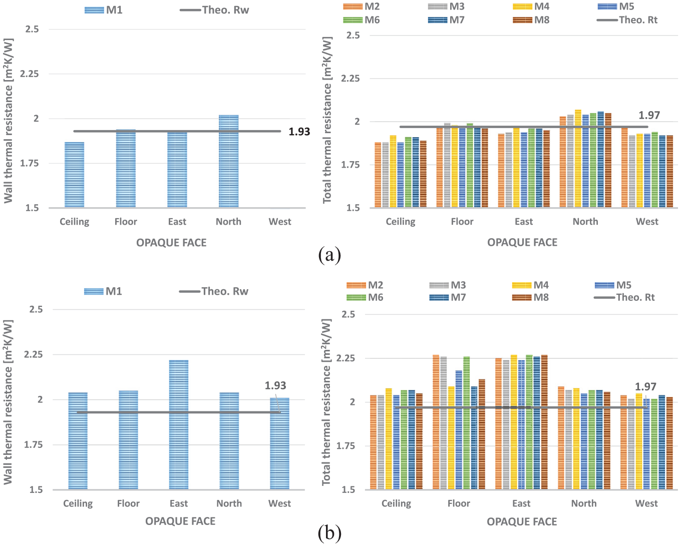
The corresponding opaque face and total thermal resistance values for each model for the selected periods in [m² K/W]: (a) Period 1 (summer) and (b) Period 2 (winter).

Table 2.

Differences of the thermal resistances obtained using LORD (R_W for M1 and R_T for M2–M8) with respect to the corresponding theoretical values in percentages for the selected periods in summer and winter in [%].

Thermal resistance	Summer								Winter
	Period 1								Period 2
Opaque face	M1	M2	M3	M4	M5	M6	M7	M8	M1	M2	M3	M4	M5	M6	M7	M8
	R %	R %	R %	R %	R %	R %	R %	R %	R %	R %	R %	R %	R %	R %	R %	R %
Ceiling	3.1	4.6	4.6	2.5	4.6	3.1	3.1	4.1	5.7	3.6	3.6	5.6	3.6	5.1	5.1	4.1
Floor	0.5	0.0	1.0	0.5	0.5	1.0	0.0	0.5	6.2	15.2	14.7	6.1	10.7	14.7	6.1	8.1
East	0.0	2.0	1.5	0.0	1.5	0.5	0.5	1.0	15.0	14.2	13.7	15.2	13.7	15.2	14.7	15.2
North	4.7	3.1	3.6	5.1	3.6	4.1	4.6	4.1	5.7	6.1	5.1	5.6	4.1	5.1	5.1	4.6
West	–*	0.0	2.5	2.0	2.0	1.5	2.5	2.5	4.2	3.6	2.5	4.1	2.5	2.5	3.6	3.1

*

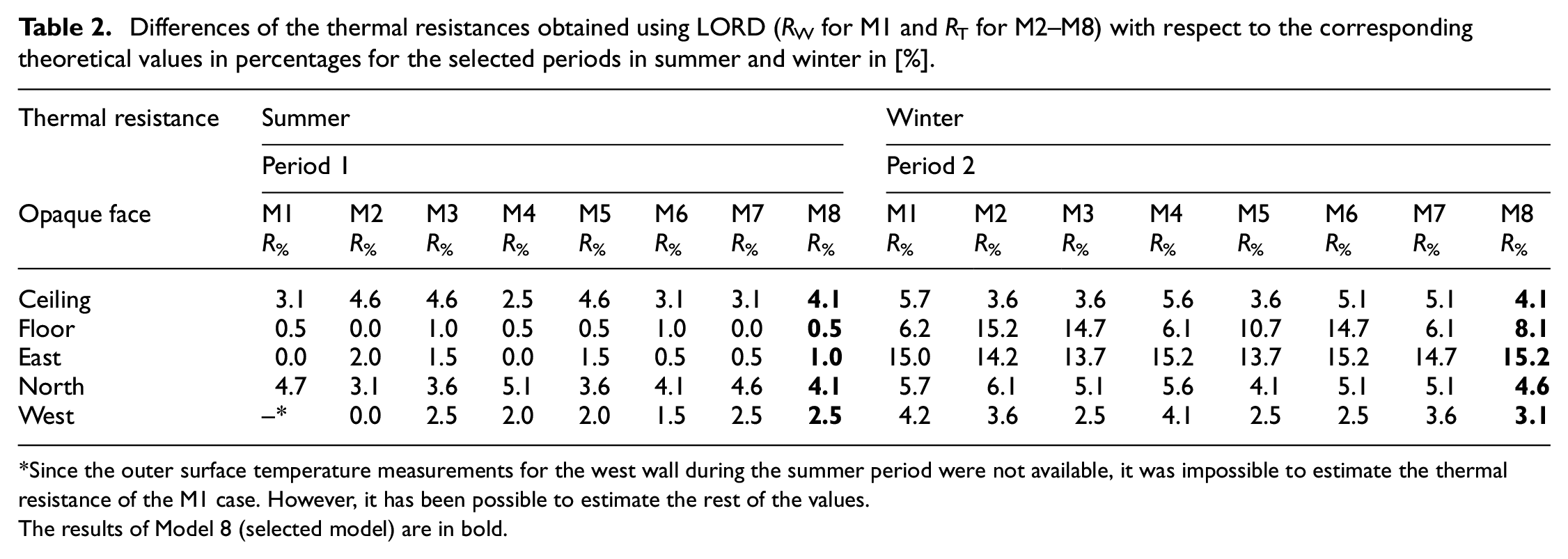
Since the outer surface temperature measurements for the west wall during the summer period were not available, it was impossible to estimate the thermal resistance of the M1 case. However, it has been possible to estimate the rest of the values.

The results of Model 8 (selected model) are in bold.

The results of Model 8 are in bold in Table 2. Interesting results can be seen in Figure 8 and Table 2. First of all, in general, the thermal resistance between all the models varies slightly, as happens with the residuals. Therefore, in some cases, it is quite complicated to select the best model based only on the identified thermal resistance value.

Taking into account the model performance observed so far, the solar absorptivity provided by the model fit has been considered for further assessment. Unfortunately, the theoretical solar absorptivity value of the walls’ outermost material was not provided. Since the outermost wall of the box is formed by fibre cement, the theoretical properties of this material can be checked and its solar absorptance reference value can be found. The solar absorptance of this material should be around 0.6 (Cengel, 2014). However, the cement fibre, being coated with white paint, could result in a theoretical solar absorptivity value close to 0.2. As a result, a theoretical solar absorptivity range between 0.2 and 0.6 will be taken into consideration. Therefore, this range can be used as a theoretical reference to discard values that are too far from it. Moreover, in order to follow physical laws, we can ensure that the estimated solar absorptivity values are not too close to zero or one and that they should provide similar values for all the façades. Therefore, Table 3 shows the solar absorptivity values obtained for the selected best models regarding the residuals of Figure 7.

Table 3.

The solar absorptivity values for the different models and opaque faces for the selected periods in summer and winter.

Opaque face surface	Summer		Winter
	Period 1		Period 2
	A5 for M5 or M6	A5 for M8	A5 for M5 or M6	A5 for M7 or M8
Ceiling	–	0.47	0.48	0.49
Floor	0.34	0.60	–	0.65
East	0.56	0.60	0.34	0.40
North	0.54	0.54	0.87	0.60
West	0.31	0.42	0.97	0.60
Average	0.44	0.52	0.67	0.55

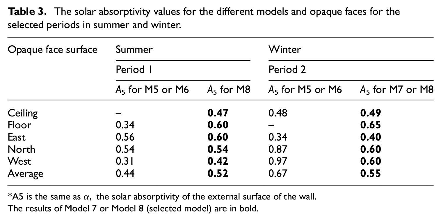
*A5 is the same as $\alpha ,$ the solar absorptivity of the external surface of the wall.

The results of Model 7 or Model 8 (selected model) are in bold.

For the M8 ceiling case in summer, the obtained value is between 0.2 and 0.6 and it is quite far from the limits, so it is directly considered to be the best model. The same procedure must be followed with the remaining models in summer. For example, in the case of the east, the floor, the west and the north walls, values inside the ranges are also obtained for Model 6 and 8. However, as discussed before, since Model 8 is the most detailed model and it provides good and consistent results for all, this is selected for all the walls for the remaining calculations in the summer period.

However, if winter results are analysed, it can be seen that there is a considerable difference between the thermal resistance values in the floor results in Figure 8. Therefore, although the best residuals were obtained for models 2, 3, 5, 6 and 8 (see Figure 7), the thermal resistance values obtained for these models, together with the solar absorptivity, are illogical. Therefore, since Model 7 was the only model to provide thermal resistance and solar absorptivity results similar to the theoretical values and the obtained residuals are not far from the lowest residuals of the rest of the models of the wall, it has been selected as the best model. In the rest of the walls, the model selection has been performed considering the solar absorptivity value as reference. In other words, the models providing solar absorptivity values too close to the identification range limits (0 as the lowest and 1 as the highest) were discarded. Once again, the selected best models are the most detailed, Models 7 and 8. Thus, it can be concluded that the most detailed models also show the best performance of the residuals and the closest physical parameters to reality. The selected model thermal resistance values are shown in Figure 9. Moreover, further insights concerning the best-fitted models are graphically presented in Appendix B. There, relevant variables of the ceiling and north wall model cases are plotted (Figures B1, B3, B5 and B7), showing the best fit obtained for each of the walls in the summer and winter periods and their RMSE values.

Figure 9.

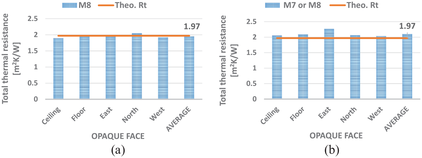
The obtained total thermal resistances (R_T values) for the selected periods: (a) Period 1 (summer) and (b) Period 2 (winter).

Therefore, for the selected models, the average estimated thermal resistance for the summer period is 1.95 m² K/W for M8. As can be seen, all values are very close to the theoretical value, 1.97 m² K/W. Moreover, if the results are analysed independently, the lowest thermal resistance value is 1.89 m² K/W and the highest is 2.05 m² K/W. The lowest value is obtained from the surface most exposed to the sun, the ceiling of the box. However, the highest value is obtained for one of the walls least exposed to the sun, the north wall. Moreover, it is well known that the average temperature of the insulation layers of a wall can affect its thermal resistance value. If the average temperature of the insulation layer increases, its thermal conductivity also increases. Thus, the thermal resistance will be reduced. Then, since the average temperature of the insulation layer can increase due to the direct effect of the solar radiation on the ceiling, the thermal resistance value can be reduced slightly. However, the opposite happens when analysing the north wall.

The same occurrence happening in this north wall can also be seen when analysing the winter results. The colder temperatures tend to cool down the average temperature of the insulation layer of the wall. Thus, the thermal conductivity of the insulation layer is reduced slightly and the thermal resistance value consequently increases. Thus, the average value of the estimated six thermal resistances of the surface to air models is slightly higher than the theoretical one and is 2.10 m² K/W.

The results obtained in this section led us to the conclusion that, although LORD is a simple and user-friendly system identification and simulation tool, it is still able to accurately estimate the physical parameters for models considering non-linear surface phenomena.

Inner surface heat flux difference results

Having proven that the model selected as the best representation of reality for each of the walls for the summer and winter periods is able to provide a proper fit of the inner surface heat flux and a good validation of the thermal physical parameters, it is then possible to carry out the rest of the calculations. Thus, the models fitted and selected in the previous section for each of the walls are taken and, once all the parameters have been fixed, the signal where the solar irradiance is included is removed from the model. Therefore, the model is then able to simulate the hypothetical inner surface heat flux ( $\overline{\stackrel{·}{q}\prime }$ ) without considering the solar radiation effect.

It has thus been possible to carry out a deeper analysis of the solar radiation effect on the inner surface heat flux. Therefore, the period averaged inner surface heat flux difference between the estimated inner surface heat flux, considering the effect of the solar radiation and without considering its effect, can be estimated. Moreover, the percentage of difference between them has also been estimated to see whether the solar radiation effect on the inner surface heat flux is negligible or not. Even if we have the real inner surface heat flux measurement, for this comparison, both inner surface heat fluxes have been obtained from the model, so any disturbance generated by the model will be identical in both inner surface heat fluxes and will not affect the calculation of the difference.

In this point, it can be stated that no step of the applied procedure is case dependent, as the characteristics of the case study do not introduce any constraint in this procedure; it could be applied to other case studies, provided the same variables used for the modelling analysis are available. Thus, the proposed procedure to assess the effect of the solar radiation on the inner surface heat flux is case independent. Accordingly, it could be applied to case studies including massive walls. Of course, for massive walls, the identified thermal capacities of the models would be much higher in order to be able to properly model the lag effect the thermal mass would produce on the inner heat flux due to solar radiation.

Figure 10(a) and (b) show the averaged inner surface heat flux, both considering and not considering the solar radiation effect, for the analysed period. It can be seen that almost all the averaged inner surface heat fluxes considering the solar radiation effect show similar results for the same period. In the case of period 1 in summer, all the average values are around 8 W/m². However, in the case of period 2 in winter, almost all of them are close to 10.5 W/m², except for the ceiling. This is slightly higher with an average inner surface heat flux value of 12 W/m². However, for the hypothetical averaged inner surface heat flux without considering the solar radiation effect, the ceiling shows a considerable difference if compared to the rest of the opaque faces in summer. Nevertheless, during the winter period, the obtained average value for the ceiling is slightly higher than the rest of the values, but the difference is not that considerable.

Figure 10.

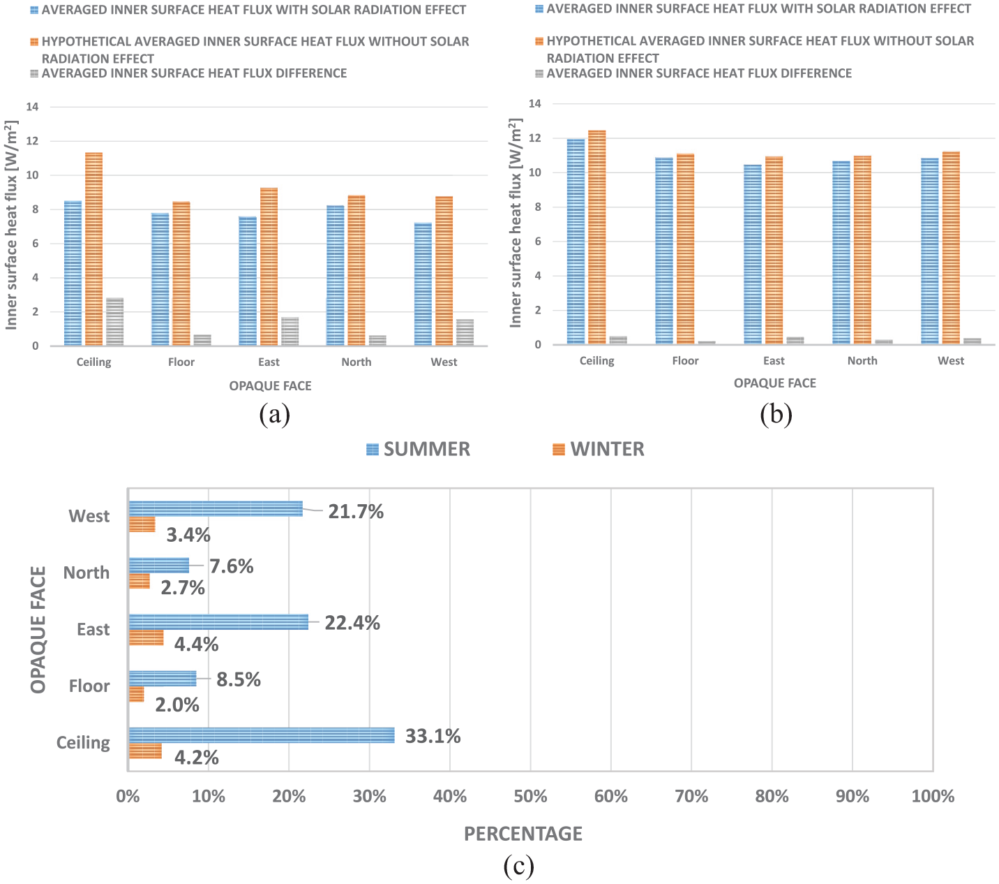
The averaged inner surface heat fluxes, the averaged inner surface heat flux difference for each period and the corresponding percentage results: (a) Period 1 (summer), (b) Period 2 (winter) and (c) The corresponding percentage results.

Figure 10(a) and (b) also shows the period averaged inner surface heat flux difference between the estimated average inner surface heat flux with and without considering the solar radiation effect. For the summer case, interesting conclusions can be taken from this Figure 10(a) and (b). As expected, since the ceiling is the most exposed to the global solar radiation effect, it is the opaque element that shows the highest inner surface heat flux difference due to this effect. After the ceiling, the east and west walls show lower values which are quite similar to each other. Finally, the north wall and the floor are the least exposed to the global solar radiation effect; so, in consequence, the difference between considering or not the solar radiation effect is the smallest. The cold and cloudy winter case is quite different when compared to the hot and sunny summer case. Since the selected winter period consists of cloudy days where mainly diffuse solar irradiance is present, the difference between all the analysed walls is very small. Remember that diffuse solar irradiance can be considered similar for all orientations.

Figure 10(c) shows the difference of the solar radiation effect on the inner surface heat flux during both the summer and winter in percentages. During summer, in opaque faces such as the ceiling, the east and the west, the effect this solar radiation has on the inner surface heat flux is considerable. However, in the rest of the opaque faces, the percentage shows quite low values. In general, this percentage is low in all the opaque faces during winter. In order to see the difference visually, Figures C1, C2, C3 and C4 of Appendix C graphically show the evolution of the inner surface heat flux (with and without solar radiation effect).

The effect of the ceiling is also enhanced by the low sky temperatures the ceiling faces during the night (see Figures B2, B4, B6 and B8 of Appendix B). It is during the nights that the ceiling faces a much colder surrounding temperature than the vertical walls on its outermost surface.

Note that this percentage of Figure 10(c) is directly proportional to the temperature difference between the outer and inner surfaces. If the temperature difference is reduced, the percentage effect of the solar radiation on the inner surface heat flux increases. The averaged inner surface heat flux, when considering solar radiation, could also be estimated by $\overline{\stackrel{·}{q}}=\frac{\overline{T_{\mathrm{Sin}}}-\overline{T_{\mathrm{Sout}}}}{R_{\mathrm{cond}}};$ while the hypothetical averaged inner surface heat flux, without considering the solar radiation effect, could be estimated by $\overline{\stackrel{·}{q}\prime }=\frac{\overline{T_{\mathrm{Sin}}}-\overline{T_{\mathrm{Sout},\mathrm{nosolar}}}}{R_{\mathrm{cond}}}$ (for long enough periods these equations provide nearly steady-state results). Here, due to the solar radiation effect, the T_Sout tends to be considerably higher than T_Sout,nosolar, which results in the $\overline{\stackrel{·}{q}\prime }$ being higher than $\overline{\stackrel{·}{q}}$ , as already shown in Figure 10. The rest of the variables and parameters used in the equations (T_Sin and R_cond) are the same for both inner surface heat flux estimations. However, the variation of the inner surface temperature in both equations can result in considerable variations in the weight that the solar radiation has on the inner surface heat flux. A simple steady-state example is performed to see this effect. If the inner surface average temperature of the wall is 40 °C, the wall’s outer surface average temperature is 20 °C and the thermal resistance of the wall is 2 m² K/W, the obtained $\overline{\stackrel{·}{q}}$ value would be 10 W/m². Then, if the T_Sout,nosolar is 18°C, the $\overline{\stackrel{·}{q}\prime }$ value obtained would be 11 W/m². Thus, the weight the solar radiation has on the inner surface heat flux, estimated using equation (22), is 10%, since the $\overline{\stackrel{·}{q}\prime }-\overline{\stackrel{·}{q}}$ value is 1 W/m² and $\overline{\stackrel{·}{q}}$ is 10 W/m². However, if the inner surface temperature is reduced to 30 °C, the temperature difference is also reduced, while the new $\overline{\stackrel{·}{q}}$ and $\overline{\stackrel{·}{q}\prime }$ are reduced to 5 W/m² and 6 W/m², respectively. Then, despite the $\overline{\stackrel{·}{q}\prime }-\overline{\stackrel{·}{q}}$ value still being 1 W/m², the $\overline{\stackrel{·}{q}}$ is considerably reduced to 5 W/m², which means the effect the solar radiation has on the inner surface heat flux will increase to 20%, double the previous case.

So, taking into account these results, a more or less relevant influence of the solar radiation can be found, depending on the indoor and weather conditions of the case study. For example, the combination of low indoor to outdoor air temperature differences and high levels of solar radiation would lead to a high impact of the solar radiation on the indoor heat flux; while this effect would be low for the combination of high indoor to outdoor air temperature differences and low levels of solar radiation.

It is also important to include the fact that, according to the uncertainty of the heat flux sensor, any effect of the solar radiation on the indoor heat flux under 5% could be hidden by the uncertainty of this measurement, which is 5% (for example, the effect on all the walls in the considered winter period). However, differences above this value would be detectable (for example, the effect on all the walls in the considered summer period).

g-value_wall estimation results

Following the procedure described above, the g-values of all the walls for both analysed periods have been obtained directly from the software used for model fitting and simulation (LORD) and from the application of equation (16). Furthermore, a theoretical g-value_wall range using equation (15) is also estimated as a reference, based on the known physical characteristic of the analysed walls. All these values are represented as follows in Figure 11:

Figure 11.

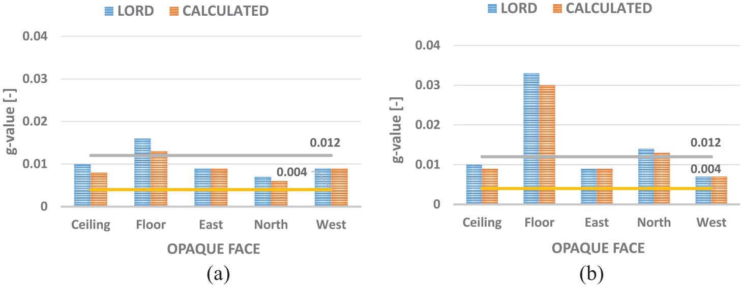
The obtained g-values_wall for each of the periods using model M7/M8 (LORD) and equation (16): (a) Period 1 (summer) and (b) Period 2 (winter).

From Figure 11, it can be concluded that, in general, the solar factor in the opaque elements is very low compared to the typical solar factor values obtained for such semi-transparent components as windows, where the solar factor is usually between 0.2 and 0.7. This result is consistent with the theoretical calculation presented in Jiménez (2016). Moreover, given the unknown theoretical value of solar absorptivity for white-painted cement fibre, the decision was made to operate within a dependable data range. Based on Figure 11, it can be observed that the vast majority of the obtained g-values fall within this range. Then, in general, the results obtained appear highly promising.

For the winter case, in the floor, the g-value_wall shows quite high values compared to the rest. This alteration in the results could be due to the extremely low solar irradiance values striking the outermost surface of the floor, which means the results are estimated with a considerably high uncertainty.

However, it has already been proven that, despite the g-values_wall being low, the effect the solar radiation has on the inner surface heat flux can be considerable for some of the cases. Finally, it must be mentioned that the results obtained using LORD and from equation (16) are very similar for all the selected models.

Conclusions

This paper proves the validity of the proposed experimental method, based on inverse modelling (with real, measured data). The method is able to accurately model the dynamic behaviour of the opaque building envelope elements through the estimation of the solar radiation effect on the inner surface heat flux and the g-value. It has been tested on the opaque elements of a carefully monitored Round Robin Box that represents a building on a small scale.

In summary, this method is applicable without the need to know in detail such thermal parameters of the envelope as the outermost surface solar absorptivity or the combined convection-radiation heat transfer coefficient. It is sufficient just to measure such variables as the inner surface temperature, the inner surface heat flux, the outer surface temperature, the outdoor air temperature, the wind speed and the corresponding global solar irradiance for each surface. In this case, some of the theoretical thermal and construction parameters of the envelope were known and have been used for reference and the validation of the models.

During the analysis of the opaque walls of the Round Robin Box, as well as the ceiling and floor, two very extreme periods have been tested. The first started on 18th June 2013 and ended on 26th June 2013. As expected, the solar irradiance was high during this summer period. However, the second period started on 19th December 2013 and ended on 21st December 2013. In this case, a cloudy period was selected in order to have a data series with the lowest possible solar irradiance. Thus, it could be ensured that the solar irradiance was almost purely diffuse and similar in all orientations.

If we look at the g-values_wall obtained for the summer period, it can be seen that the results are very low compared to the typical solar factors estimated for windows. However, if the effect of the solar radiation on the inner surface heat flux is observed, it can be concluded that its effect cannot be neglected for some of the opaque envelope elements. In the case of the Round Robin Box’s ceiling, the reduction of the inner surface heat flux due to the solar radiation effect was 33.1%. Moreover, the effect on the east and west walls is also considerable, with 22.4% and 21.7%, respectively. As the north wall and the floor are the least exposed to solar radiation, the effect in these is considerably lower.

However, in the case of the winter period, the results are completely different, if compared to the summer case. Although the g-values for the opaque faces are also low, as in the summer period, the effect of the solar radiation on the inner surface heat flux is considerably lower. In this case, the effect obtained in winter for the ceiling is 4.2%, very similar to the east and west wall results, 4.4% and 3.4%, respectively. In this case, the lowest values are also obtained for the floor and the north wall, with effects of around 2%.

If the effect of the solar radiation on the inner surface heat flux is significant, as happens in some opaque envelope elements during the summer period, not considering the blocking effect of the outwards heat flux leads to an underestimation of the Heat Loss Coefficients (HLC) estimated by methods where the solar gains are not estimated as an identifiable value. From the results, it can be concluded that not considering the solar gains effect through the opaque walls in cold and cloudy periods could be negligible in the estimation of the HLC value. However, this is not true for sunny periods.

Finally, it must be remarked that, although the LORD system identification software could be considered a relatively simple tool, it has been able to deal with non-linear surface phenomena occurring in the outermost surface of the analysed walls. It can therefore be concluded that the software is able to work with complex and detailed models, providing suitable and reliable results.